基於 SURE 之最佳化的自適應採樣與重建技術

(1)

國立臺灣大學電機資訊學院資訊工程學系碩士論文

Department of Computer Science and Information Engineering College of Electrical Engineering and Computer Science

National Taiwan University Master Thesis

基於 SURE 之最佳化的自適應採樣與重建技術 SURE-based Optimization for Adaptive Sampling and

Reconstruction

李子懋 Tzu-Mao Li

指導教授：莊永裕博士 Advisor: Yung-Yu Chuang, Ph.D.

中華民國 102 年 6 月 June, 2013

(2)

Acknowledgements

There are many people to thank for their help on this thesis. First I would like to thank my advisor Yung-Yu Chuang who initiates my motivation to explore the wonderful world of rendering. I found that his astute and insightful advices are very helpful and his sense of humor always brings laughters and happiness to people around him.

Next I would like to thank my colleague Yu-Ting Wu. The work would not have been possible without the stimulus discussions with him.

His hard-working attitude also aﬀects me a lot. Without him, my grad- uate student life would have been completely diﬀerent.

Regards go to the members of CMLab who made my life more en- joyable for all the fun chatting and the memorable moments. Listing all of them here will occupy too much space, while listing only part of them can be unfair to the people who are not listed, so I choose to not list the names here.

Although we have not met yet when I am writing this thesis draft, thanks for my thesis committee members, Chih-Yuan Yao, Chun-Fa Chang, Yu-Chi Lai, Yu-Ting Tsai(sorted by alphabetic order), for willing to be the committee member, and taking time to review the thesis.

Thanks for the anonymous SIGGRAPH Asia reviewers for their valu- able comments and accepting our paper.

Thanks for the people who created the wonderful tools and elements that I have used during writing this thesis. For a few examples: Tz- Huan Huang who made the NTU thesis template, Matt Pharr and Greg Humphreys who built the renderer pbrt, and numerous modellers who created the models used in the rendered image.

Thanks for the people who have developed countless beautiful and as- tonishing theorems and algorithms in both the ﬁeld of mathematics and computer science, especially those who have contributed to the fascinat- ing realm of rendering. These people have constructed a lovely world that deeply attracts me and has profound eﬀect on my life.

Finally and most importantly, thanks my parents for their love and support.

This acknowledgement is purposely written in English so that I can impute my poor writing skill to a non-native language.

(3)

摘要

本論文提出了一個利用 Stein’s Unbiased Risk Estimator (SURE) 的自適性採樣與重建演算法，以應用在蒙地卡羅影像渲染上。SURE 是一個在統計上對均方差的無偏估計，利用 SURE，我們可以估計任意一種重建濾波器所造成的誤差，使得我們可以使用更有效率的濾波器，

例如使用輔助特徵圖的交叉雙邊濾波器 (cross bilateral ﬁlter) 或是非局域均質濾波器 (non-local means ﬁlter)，而非過去的方法所限制的對稱濾波器；此外，SURE 也可以讓我們對估計出較高錯誤的區域使用更多樣本。由此我們可以建立一個最佳化 SURE 的自適性採樣與重建系統。本論文另外也提出一個對記憶體較友善的方法來減少景深與物體或視點移動造成的雜訊對用來輔助濾波的特徵圖的干擾。實驗顯示本論文提出的方法相較於之前的方法在同樣的時間內可產生更清晰，但較少雜訊的圖片。

(4)

Abstract

This thesis presents a method applying Stein’s Unbiased Risk Esti- mator (SURE) to adaptive sampling and reconstruction to reduce noise in Monte Carlo rendering. SURE is a general unbiased estimator for mean squared error (MSE) in statistics. With SURE, we are able to estimate error for an arbitrary reconstruction kernel, enabling us to use more effective kernels, such as cross bilateral filters utilizing auxiliary feature buffers or non-local means filter, rather than being restricted to the symmetric ones used in previous work. It also allows us to allocate more samples to areas with higher estimated MSE. Adaptive sampling and reconstruction can therefore be processed within an optimization framework. We also propose an efficient and memory-friendly approach to reduce the impact of noisy geometry features where there is depth of field or motion blur. Experiments show that our method produces images with less noise and crisper details than previous methods.

(5)

List of Figures

1.1 Comparisons between GEM and our method with kernel visualization 1

4.1 An overview of our algorithm . . . 10

4.2 Comparisons of our normalized distance and L2 distance . . . 12

4.3 Visualization of the scale selection map . . . 13

4.4 Visualizations for the sampling density of our approach. . . 15

5.1 A comparison on the SIBENIK scene . . . 23

5.2 A scene with a glossy teapot . . . 24

5.3 Comparisons on a complex scene SPONZA . . . 25

5.4 Comparisons on the TOWN scene . . . 26

5.5 Error visualization . . . 27

5.6 The proposed SURE-based framework incorporated with an isotropic Gaussian ﬁlterbank and compared with GEM [26] . . . 28

5.7 Comparison of cross non-local means ﬁlters without and with SURE- based framework . . . 29

(8)

List of Tables

5.1 Rendering statistics . . . 17

(9)

Chapter 1 Introduction

Figure 1.1: Comparisons between greedy error minimization (GEM) [26] and our SURE-based filtering. With SURE, we are able to use kernels (cross bilateral filters in this case) that are more effective than GEM’s isotropic Gassians. Thus, our approach better adapts to anisotropic features (such as the motion blur pattern due to the motion of the airplane) and preserves scene details (such as the textures on the floor and curtains). The kernels of both methods are visualized for comparison.

Monte Carlo (MC) integration is a common technique for rendering images with distributed effects such as antialiasing, depth of field, motion blur, and global illumination. It simulates a variety of sophisticated light transport paths in a unified manner; it estimates pixel values by using stochastic point samples in the integral domain. Despite its generality and simplicity, however, the MC approach converges slowly. A complex scene with multiple distributed effects usually requires several thousand expensive samples per pixel to produce a noise-free image.

(10)

thesis) are two effective techniques for reducing noise. Given a fixed budget of samples, adaptive sampling determines the optimal sample distribution by concen- trating more samples on difficult regions. To decide which pixels are worth more effort, we require a robust criterion for measuring errors. Accurate estimation of errors is challenging in our application because the ground truth is not available.

Reconstruction algorithms, in contrast, properly construct smooth results from the discrete samples at hand. One key issue that reconstruction must resolve is how to select the filters for each pixel, as the optimal reconstruction kernels are usually spatially-varying and anisotropic. Recently, approaches have been developed to address the challenge of spatially-varying filters [6, 26], producing better results than those that use a single filter across the whole image. However, these methods are limited to symmetric filters and do not work well for scenes with anisotropic features such as high-frequency textures on the floor and curtains in Figure 1.1.

We here propose an adaptive sampling and reconstruction algorithm to improve the efficiency of Monte Carlo ray tracing. The core idea is to adopt Stein’s Unbi- ased Risk Estimator (SURE) [31], a general unbiased estimator for mean squared error (MSE) in statistics, to determine the optimal sample density and per-pixel reconstruction kernels. The advantages of using SURE are twofold. For one, it provides a means by which to measure the quality of arbitrary reconstruction kernels – not just those that are symmetric (e.g. isotropic Gaussians used in greedy error minimization (GEM) [26]). As such, it allows for the use of more effective filters such as cross bilateral filters and cross non-local means filters. Another advantage is that the per-pixel errors estimated by SURE can be used to guide further sample distribution. Thus more samples can be allocated to difficult regions. In addition to applying SURE, we propose an efficient and memory-friendly approach to maintain the quality of cross bilateral filtering in the presence of noisy geometric features when rendering depth-of-field or motion blur effects. We propose a normalized distance to alleviate the impact of noisy features, making the proposed method more robust to all types of distributed effects. Experiments show the proposed method

(11)

provides signiﬁcant improvements over previous techniques for adaptive sampling and reconstruction.

(12)

Chapter 2 Related work

2.1 Adaptive sampling and reconstruction

The seminal work of Mitchell [20, 21] over twenty years ago laid the foundation for methods for adaptive sampling and reconstruction. We categorize these techniques as image space methods, multidimensional methods, and adaptive ﬁltering.

Image space methods estimate per-pixel errors with various criteria and allocate additional samples to diﬃcult regions. These approaches usually are more general and can be used for various types of eﬀects. Bala et al. [1] combine edge information and sparse point samples to perform edge-aware interpolation. The quality of their results is highly dependent on the accuracy of edge detection. Overbeck et al. [23]

proposed adaptive wavelet rendering (AWR), a general wavelet-based adaptive sampling and reconstruction framework. They distinguish the sources of variances as the coarse level for distributed effects and the fine level for edges. These two types of noise are addressed separately by sampling the hierarchical wavelet coefficients adaptively; smooth images are reconstructed by thresholding wavelet coefficients.

Recently, several approaches [6, 26] have been proposed to smooth out noise using multi-scale filters. Chen et al. [6] focus on depth of field and describe a criterion to select spatially-varying Gaussian filters from a predefined filterbank based on the depth map. Rousselle et al. [26] also use Gaussian filters to form a filterbank. Al- though their method uses an error minimization framework for adaptive sampling

(13)

and reconstruction, and is more general, the framework can be used only for symmetric filters. We apply SURE to estimate MSE for more general filters and allow the use of more effective filters, which yield significant improvements.

Other approaches perform adaptive sampling and reconstruction in a multidimensional space. Hachisuka et al. [14] distribute more samples to discontinuities in the high dimensional space and reconstruct them anisotropically using structure tensors. Their approach achieves good quality but becomes less efficient as the number of dimensions increases. Approaches have also been developed that are based on transform domain analysis, focusing on specific distributed effects such as depth of field [30], motion blur [10], and soft shadows [9]. Lehitinen et al. proposed a novel method for reconstructing temporal light-field samples [15], and later extended it to handle the indirect light field for global illumination [16]. By reprojecting samples along the sample trajectories in the multidimensional space, expensive samples can be reused. In general, to avoid the curse of dimensionality, multidimensional approaches usually focus on only one or two specific effects. These methods are able to generate better results for the effects they focus on because the anisotropy of the integrand is taken into account. Our method, however, is more general, efficient, and memory-friendly. Recently there are some methods combine the analysis in multidimensional space and the efficiency in the image space [3, 18, 19] by project- ing the anisotropic high dimensional filter kernel onto image space. However, these methods are still limited to a few effects and lacks generality.

Some methods focus on reconstruction only. Xu et al. [34] proposed smoothing out Monte Carlo noise with a modiﬁed bilateral ﬁlter with smoothed range values.

Segovia et al. [27], Dammertz et al. [7], and Bauszat et al. [2] focus on interactive global illumination. They exploit geometric properties such as depths and surface normals to identify edges. Shirley et al. [29] use the depth buffer to help filtering, but target defocus and motion blur. Sen and Darabi [28] proposed a general adaptive filtering approach based on information theory. By identifying the dependencies between random parameters on sample colors and scene features, they reduce the

(14)

importance of sample values influenced by MC noise. Moon et al. [22] introduced the virtual flash image as a feature image, it would be an interesting avenue to combine their method and ours as we can apply their feature image and filter weight in our framework, and optimize the filtering parameters.

2.2 Denoising using SURE

Stein [31] proposed an MSE estimator called Stein’s Unbiased Risk Estimator (SURE) for estimators on samples with normal distributions. Donoho and John- stone [8] incorporate the estimator into a Wavelet shrinkage algorithm to reconstruct functions from noisy inputs. Recently, SURE has received much acclaim from the image denoising community and has been widely used to optimize denoising parameters [4, 25, 33].

(15)

Chapter 3 Stein’s Unbiased Risk Estimator (SURE)

Monte Carlo ray tracing estimates true pixel colors by randomly sampling the integral domain and reconstructing from samples. The unbiased Monte Carlo rendering techniques have a stochastic error bound which can be estimated using the variance of the estimator. According to the central limit theorem, if Y is the pixel color estimated by an unbiased Monte Carlo renderer and x is the true color, as the number of samples n approaches inﬁnity, Y ’s distribution approximates a normal distribution with mean x and variance σ²/n:

Y → N^d (

x,σ² n

)

, (3.1)

where σ² is the variance of the Monte Carlo samples. Previous investigations have demonstrated that, for a ﬁnite number of samples, this relationship is still a good approximation [32, 11, 13].

Since a Monte Carlo renderer is an estimator, it is often necessary to estimate its accuracy for applications such as adaptive sampling. Stein’s Unbiased Risk Estima- tor (SURE) oﬀers a means for estimating the accuracy of a given estimator [31, 4].

SURE states that, if y is a measurement on x with a normal distribution N (x, σ_y²),

(16)

and F is a weakly diﬀerentiable function, then the following estimation of error¹,

SURE(F (y)) =∥F (y) − y∥²+ 2σ_y²dF (y)

dy − σy², (3.2) is an unbiased estimator of the mean square error (MSE) of F(y)² , that is,

E[SURE(F (y))] = E[∥F (y) − x∥²]. (3.3)

Equations 3.2 and 3.3 indicate that if we can compute σ_y and dF (y)/dy, we can estimate the error of an estimator F without knowing the true underlying value x.

Our goal is to use the above formula to estimate the reconstruction error of an arbitrary kernel F . As mentioned above, rendering samples y follow a normal distribution. Thus, SURE can be used as the estimator for MSE of any filter F if we can compute dF (y)/dy for the reconstruction kernel (σy can be directly estimated from Monte Carlo samples). Chapter 4 describes details of the algorithm, including the definition of F , the derivation of dF (y)/dy, and how to use SURE for optimal filter selection and adaptive sampling.

It is worth noting that Rousselle et al. [26] attempted to estimate MSE for the same application. They decomposed the error into variance and bias and exploited the relation between the biases of the two filters to estimate the error. However, they used a quadratic approximation which is valid only for symmetric filter kernels, thus limiting the effectiveness of their approach. In contrast, our SURE-based estimation works for arbitrary reconstruction kernels and provides more flexibility to the choice of kernels.

1We followed Blu and Luisier’s SURE formulation [4], which was derived from the original SURE [31]; their equivalence has been shown. Since we apply SURE to estimate MSE errors for each color channel independently, the ﬁlter kernel F is a scalar function. Thus, the dimension is 1 and the divergence in the original SURE formulation becomes a derivative.

2Readers should not be confused between the term unbiased and unbiased rendering. Here we mean that SURE is an unbiased estimator of the MSE∥F (y) − x∥², instead of the true pixel value.

(17)

Chapter 4 Method

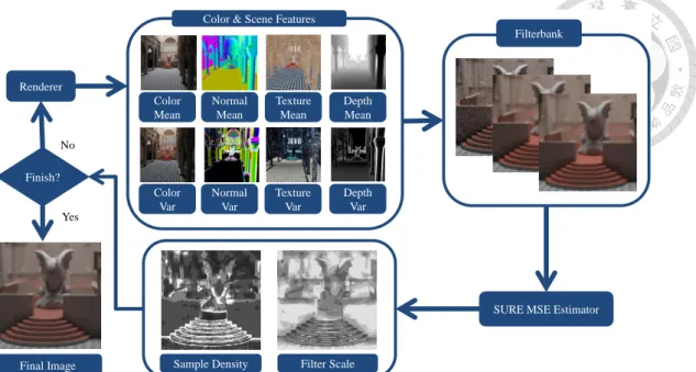
Figure 4.1 demonstrates the flowchart of the proposed method. Our method starts by rendering a small number of initial samples for each pixel and then iter- ates between filter selection and adaptive sampling stages until reaching the sample budget. After each sampling phase, we reconstruct a set of images using a filterbank. Each pixel is filtered multiple times with all candidate filters in the filterbank and the error of each filtered pixel color is estimated by computing SURE. For each pixel, the filtered color with the least SURE error is chosen and filled into the reconstructed image. If more sample budget is available, the adaptive sampling stage is invoked and a batch of new samples is distributed to pixels with larger SURE errors. Details are in the following sections.

4.1 Initial samples

At the beginning, a small number of initial samples (usually 8 or 16 samples per pixel) are taken to explore the scene. The samples are generated by low discrepancy sequences and distributed evenly to each pixel. After rendering with these samples, our method performs the ﬁrst reconstruction phase with the gathered information.

(18)

Renderer

Color Mean

Color Var

Color & Scene Features

Filterbank

SURE MSE Estimator

Filter Scale Sample Density

Finish?

No

Yes

Normal Mean

Normal Var

Texture Mean

Texture Var

Depth Mean

Depth Var

Final Image

Figure 4.1: An overview of our algorithm, which alternates between sampling and reconstruction until reaching the sample budget. During sampling, a set of samples collects colors, normals, textures and depths over the image plane. They are used as the side information for filters in the reconstruction stage, during which, for each pixel, a set of filters are performed and the filtered value with the minimal SURE value is filled into the reconstructed image. In addition, the minimal SURE value of each pixel is recorded to guide adaptive sampling. If there are sample budgets left, more samples are shot for pixels with larger SURE errors.

4.2 Filter selection using SURE

The main advantage of our method over greedy error minimization [26] is its ability to use arbitrary filters. We have experimented with three different filters:

isotropic Gaussian, cross bilateral, and a modified non-local means filter [5] with additional scene feature information (we call this a “cross non-local means filter”;

see Section 5.4). Here, we use the cross bilateral filter as an example since it offers the best compromise between performance and quality amongst these filters. Algorithms for different filters are the same except that different filters are used for constructing the filterbank; the derivatives in SURE are different also.

Cross bilateral filters. Cross bilateral ﬁlters have been shown eﬀective for remov- ing Monte Carlo noise [7, 28]. Similar to previous work, auxiliary data including surface normals, depths, and texture colors are collected by caching information af-

(19)

ter tracing rays. We compute the per-pixel mean and variance of each feature and store them as feature vectors for cross bilateral filters. For the cross bilateral filter, the filter weight w_ij between a pixel i and its neighbor j is defined as

w_ij = exp(−∥pi− pj∥²

2σs2 ) exp(−∥ci− cj∥² 2σr2 )

∏m k=1

exp(−D( ¯f_ik, ¯f_jk)²

2σf_k2 ), (4.1)

where ¯f_ik is the sample mean of the k-th feature for the pixel i; σ_s, σ_r, and σ_f_k are the standard deviation parameters of the spatial, range (sample color), and feature terms respectively. D is a distance function used to address noisy scene features for depth of ﬁeld and motion blur. It will be discussed later in this section. The ﬁltered pixel color ˆc_i of the pixel i is computed as the weighted combination of the colors c_j of all neighboring pixels j:

ˆ c_i =

∑n

j=1wijcj

∑_n

j=1w_ij . (4.2)

Note that the cross bilateral kernels are spatially-varying due to the range and feature terms. Figure 1.1 shows examples.

In our current implementation, the filterbank is composed of cross bilateral filters with different σ_s, corresponding to different spatial scales. Other parameters σ_r and σf_k are fixed and their values are discussed in Chapter 5.

Depth of field and motion blur. Sen and Darabi [28] point out that when render- ing depth of field and motion blur effects, the geometric features (texture, surface normal and depth) can be noisy due to MC noise. In these situations, as the weight- ing function is not accurate, using the features dogmatically for filtering can fail to remove the noise or oversmooth the image. They resolve this problem by computing the functional dependency of the MC random parameters and the scene features and using it to reduce the weight of samples if their features are highly dependent on the random parameters. Although their method successfully handles depth of field and motion blur, it operates at the sample level. Thus, performance and memory consumption become issues since computing pairwise mutual information between samples and parameters is not only time-consuming but also requires considerable

(20)

(a) PLANE (b) Texture (c) Texture var (d) MC 8 spp

(e) Normalized dist. (f) L2 dist. low σ_{f k} (g) L2 dist. high σ_{f k} (h) Reference Figure 4.2: Comparisons on filtering the PLANE scene with depth-of-field effects using our normalized distance and L2 distance. The lefttop image is reconstructed by our method, and the reference image is generated by using 8192 samples per pixel. The out of focus plane contains noisy texture information. If we use a lower σ_{f k}, the back plane will be noisy because the texture feature itself is noisy. On the other hand, if we use a higher σ_{f k}, the front plane will be too blurry because we are in effect ignoring the texture feature. By incorporating sample variances, normalized distance allows us to filter the out of focus plane while preserving the texture on focus plane even given noisy geometry information. Note that the large texture variances on the out of focus area in (c) allow us to effectively reduce the weight of noisy features, removing the artifacts exhibited in the result with L2 distance (f) (g).

memory for storing samples.

We propose a more efficient and memory-friendly approach to prevent cross bilateral filters from being affected by noisy scene features. Each pixel has a set of samples for feature k. Given two pixels i and j, to measure their distance with regard to the feature, the naive metric would be the Euclidean distance between the sample means, ¯f_ik and ¯f_jk. This, however, completely ignores sample variances.

If we model samples as Gaussians, the distance between two sample sets should be normalized by their variances. Thus we deﬁne the normalized distance as

D( ¯f_ik, ¯f_jk) =

√∥ ¯f_ik− ¯f_jk∥²

σ_ik² + σ²_jk , (4.3)

(21)

(a) gargoyle (b) selection map (c) Global (d) Our (e) Reference MSE: 1.17E-2 MSE: 2.15E-3

Figure 4.3: Visualization of the scale selection map for σ_s of our method. We have also compared our approach to a global cross bilateral filter (which uses the same scale parameter, the largest σ_s in the filterbank, for all pixels). It is clear that the global cross bilateral filter produces large bias in the shadow areas. Our approach adapts better and uses fewer samples in these areas, thus leading to a smaller error.

The sampling rate of the noisy input image is about 32 samples per pixel.

where σ_ik² and σ²_jk are sample variances of the k-th feature of pixels i and j respec- tively. Intuitively, for a pixel with strong depth of field and motion blur, its samples tends to have a large variance since these samples usually span over a large region in the spatial-temporal domain. Thus, it tends to have smaller distances and larger weights even when the geometric features are far apart. In the extreme case that two feature sets are inseparable due to strong depth of field or fast motion, the cross bilateral filter reduces to a Gaussian filter and does not use the unreliable geometric features. This approach allows us to evaluate feature importance at the pixel level and store only the sample mean and variance of features per pixel. This normalized distance is related to the Mahalanobis distance [17] with the assumption of indepen- dent feature noise, which results in a diagonal covariance matrix. Figure 4.2 shows the effect of the proposed distance metric.

Computing SURE and selecting the per-pixel optimal filter. For each pixel, we need to use the minimal SURE error to determine the optimal scale for the cross bilateral filters in the filterbank. As mentioned in Chapter 3, in calculating SURE, we need to compute dF (ci)/dci for the cross bilateral filter F defined in Equation 4.2.

We have obtained its analytic form as

dF (c_i)

dc_i = 1

∑_n

j=1w_ij + 1

σ_r²(F²(c_i)− F (ci)²), (4.4)

(22)

where

F²(c_i) =

∑_n

j=1w_ijc_j²

∑_n

j=1w_ij . (4.5)

The derivation is in Appendix A. We then compute SURE to estimate the MSE for each filter in the filterbank using Equation 3.2. For each pixel, the filter with the least SURE error is selected and its filtered color is used to update the pixel.

We have observed that computing SURE using MC samples usually leads to noisy filter selection and thus yields noisy results. This is because SURE is an unbiased estimator of MSE and has its own variances. To reduce variances, one can either add more samples or perform filtering. For the sake of efficiency, we opted to perform filtering to reduce the variances of SURE. To be more concrete, we prefilter the estimated MSE image using a cross bilateral filter with a fixed parameter before SURE optimization. A similar problem was encountered in the previous method [26];

they smoothed out the selected scales of ﬁlters to deal with the variance of their estimator.

Figure 4.3 shows the scale selection map and compares our SURE-based ﬁlter- ing with a global cross bilateral ﬁlter (with the same scale for each pixel). It is obvious that spatially-varying scale selection yields better results both visually and quantitatively.

4.3 Adaptive sampling

The MSE estimated using SURE can be taken as feedback to the renderer; the sampling density should be proportional to the estimated MSE. However, since our MSE estimation is not perfect (note that Equation 3.2 can be negative), a heuristic variance term is included to ensure that regions with higher variances are allocated more samples. In addition, to guide more samples to darker areas, we scale our sampling function with the squared luminance of the ﬁltered color. This strategy was also adopted by a previous approach [23] because human eyes are more sensitive to error in dark regions. As a result, the sampling function for a pixel i is determined

(23)

Sampling density Reconstructed image Figure 4.4: Visualizations for the sampling density of our approach.

by

S(i) = SURE(F (c_i)) + σ_i²

I(F (c_i))²+ ϵ , (4.6)

where σ²_i is the variance of samples within the pixel, I(F (c_i))² is the squared lu- minance of the ﬁltered pixel color, and ϵ is a small number used to prevent a null denominator (set to 0.01). If the current sampling budget is m, pixel i receives

⌈mS(i)/∑

jS(j)⌉ samples. Just like the scale selection map, the sampling map can also be noisy, and we also filter the sampling map with the same fixed cross bilateral filter. Figure 4.4 visualizes the sampling density for two examples. It is clear that samples concentrate on areas with geometry or texture details, discontinuities, or more noise.

(24)

Chapter 5 Results and discussions

We implemented the algorithm on top of the PBRT2 system [24]. All results were generated on a machine with an Intel dual quad-core Xeon E5420 CPU at 2.5GHz, 32GB of RAM, and using 8 threads. As mentioned, we mainly used cross bilateral ﬁlters in the proposed SURE-based framework. In Section 5.4 we discuss results with other ﬁlters.

5.1 Parameter setting

There are a number of parameters for the features in Equation 4.1. They were set as σ_{f k} = 0.8 for normal, σ_{f k} = 0.25 for texture color, and σ_{f k} = 0.6 for depth throughout all experiments. We did not use σr in our current implementation since in practice we found the color term in the cross bilateral filter does not help much. We varied the spatial scale parameter σ_s to form the filter- bank. We used σ_s = 1, 2, 4 to construct the filterbank in intermediate iterations and σ_s = 1,√

2, 2, 2√

2, 4, 4√

2, 8 for the final reconstruction. We used fewer filters for intermediate phases as we found it sufficient and more efficient. Experiments show this setting strikes a good compromise between performance and quality. For the parameters used in prefiltering before SURE computation, we set σ_s = 8, and the same σf k as mentioned above. In practice, results are not very sensitive to these parameters and a wide range of parameters work equally well. Although parameters

(25)

SIBENIK TEAPOT SPONZA TOWN MC

spp 44 35 68 82

time 140s 42s 890.5s 59.9s

rel. MSE 2.99E-2 1.99E-1 1.33E-1 2.98E-2 GEM

avg. spp 39.86 23.96 63.84 51.82

time 135s 44.3s 906.2s 61.8s

rel. MSE 2.07E-3 1.71E-1 1.76E-2 1.84E-2 RPF

spp 8 8 16 8

time 363s 374.4s 1676.1s 272.4s

rel. MSE 6.10E-3 2.34E-1 3.20E-2 5.79E-2 Our(low)

spp 8 8 16 8

time 85.1s 39.3s 280.6s 26.5s

rel. MSE 3.34E-3 1.34E-1 2.05E-2 3.24E-2 Our

avg. spp 26.48 8 62.48 38.28

time 149.3s 39.3s 893.1s 60.9s

rel. MSE 1.28E-3 1.34E-1 8.32E-3 1.12E-2

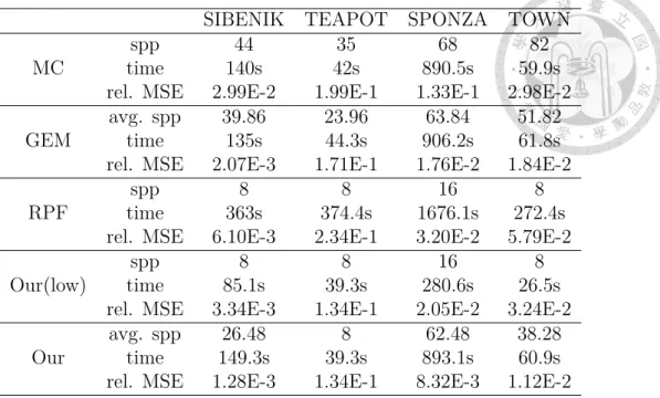
Table 5.1: Rendering statistics comparing MC, GEM, RPF, and our method. We also include an equal-sample comparison with RPF. Our algorithm consistently produces smaller error images given the same time budge compare to other methods.

In addition, the equal-sample comparison to RPF demonstrates that our method gives lower error and uses much less time.

can be ﬁne-tuned for each scene, this yields only marginal improvements.

5.2 Comparisons

We applied our algorithm on rendering four scenes – SIBENIK(1024x1024), TEAPOT (800x800), SPONZA (1600x1200) and TOWN (800x600) – with a variety of effects, including global illumination, motion blur, depth of field, area lighting, and glossy reflection (Figures 5.1 to 5.4). We have also compared our method on these scenes with the following methods:

• MC: Uniform sample distribution and per-pixel box ﬁlter. This approach is used as the baseline without adaptive sampling and reconstruction.

• GEM: Adaptive sampling and reconstruction using greedy error minimization [26]. The results were produced by the authors’ implementation on the PBRT2 system. For all scenes, we set the γ parameter in their algorithm to 0.2 as the paper suggested.

(26)

• RPF: Adaptive ﬁltering using random parameter ﬁltering [28]. We imple- mented their approach on the PBRT2 system. The σ² in their algorithm is set to 0.002 according to the authors’ suggestion.

The number of samples for each method was carefully adjusted to make equal- time comparisons. However, since RPF consumes considerable memory and time compared to other methods, its number of samples was limited to 8 or 16. For very complex scenes, the time for reconstruction could be negligible if taking samples is very expensive. To make fair comparisons under such situations, we also include equal-sample comparisons between RPF and our method. Finally, we also compared all methods quantitatively with the relative MSE proposed by Rousselle et al. [26].

It is deﬁned as the average of (y− x)²/(x²+ ϵ), where y is the estimated pixel color, x is the pixel color in the reference image, and ϵ is set to 0.01 to prevent division by zero. The rendering statistics of each method are listed in Table 5.1. We also visualize the error map of each method in Figure 5.5

Figure 5.1 compares these algorithms on SIBENIK, a scene with global illumination and depth of field. The image produced by MC retains considerable high- frequency noise even in simple areas such as the floor. GEM eliminates floor noise, while at the same time oversmoothing the area with textures due to its use of isotropic filters. Note that, although its relative MSE seems good, GEM tends to yield oversmoothed images. RPF produces a slightly sharper image than GEM but it is still oversmoothed, especially where there are depth-of-field effects. Our approach produces an image with much less noise while faithfully preserving textures.

The TEAPOT scene (Figure 5.2) demonstrates a challenging case with very high-frequency bump mapping and glossy reﬂections. None of the four methods preserve the bump map on the ﬂoor well. Again, MC produces a very noisy image.

It is also worth noting that RPF fails to reproduce the self-reﬂection on the teapot.

Overall, our approach still produces an image that is visually more pleasing and quantitatively more accurate than other methods.

(27)

The SPONZA scene in Figure 5.3 contains motion blur effects. As shown in the first row of insets, the anisotropic pattern produced by motion of the wing is more vivid in our result than in the others. In addition, our approach more faithfully preserves the textures on the floor and the curtains.

Finally the TOWN scene shown in Figure 5.4 was designed to test environment lighting, area lights, and motion blur. The scene is challenging also due to the heavy occlusion between the buildings and skyscrapers. Despite its strong MSE, GEM fails to reconstruct all the textures in the scene, which are preserved well in our results. RPF, on the other hand, produces a very noisy image. This could be related to the sampling procedure in their bilateral ﬁltering computation. Our approach outperforms the others by producing less noise and crisper details.

5.3 Discussions

GEM performs adaptive sampling and selects per-pixel filters in an attempt to minimize MSE. From the results, it does achieve lower relative errors compared to MC and RPF (and comparable to our approach). However, as mentioned, GEM is limited to symmetric filters and does not adapt well to high-frequency textures and detailed scene features. In all our test scenes, the results produced by GEM exhibit obviously oversmoothed artifacts. In addition, the GEM adaptive sampling criterion tends to send very few rays to the regions where most of the samples carry null radiance (for example, the right pillar of SPONZA in Figure 5.3). Our approach significantly alleviates these problems by using cross-bilateral filters and prefiltering MSE before SURE optimization.

RPF adjusts the weights of cross-bilateral filters by using mutual information and adapts well to scene features in most cases. It also removes the noise produced by few samples when rendering depth-of-field or motion blur effects. However, its multi-pass reconstruction algorithm can produce slightly oversmoothed results, such as the texture on the floor in SIBENIK (Figure 5.1), the disappeared shadows in

(28)

ure 5.2). Another severe limitation of this approach is that the mutual information must be computed at the sample level, making the computation ineﬃcient in both performance and memory consumption. To render one high-quality image at the 1920x1080 full HD resolution with 64 samples per pixel, it takes up to 13 GB to store the samples (108 bytes per sample as described in the paper). Finally, RPF is designed for reconstruction and does not have a feedback mechanism to the renderer for adaptive sampling.

Our method does away with the limitations of both GEM and RPF. At one end, we adopt SURE to estimate the error of an arbitrary reconstruction kernel. This allows us to optimize over a discrete set of cross bilateral filters for each pixel and determine the optimal sample distribution. Also, we propose a memory-friendly method to detect noisy geometric features when rendering depth of field and motion blur. As a result, our method successfully eliminates MC noise for a wide range of effects while preserving high-frequency textures and fine geometry details.

5.4 Other ﬁlters

To demonstrate the flexibility of the proposed framework with respect to different filters, in addition to cross bilateral filters, we have also experimented with isotropic Gaussian filters and cross non-local means filters. For isotropic Gaussians, we compare the results with GEM [26] which is specifically designed for optimiz- ing over an isotropic Gaussian filterbank. To be fair, we filter the SURE-estimated MSE using an isotropic Gaussian filter without using scene feature information. As shown in Figure 5.6, results of both methods are comparable and the scale selection maps are similar. This means that our SURE optimization is comparable to the specifically-designed GEM for the isotropic case.

The non-local means ﬁlter [5] is a popular method for image denoising. It assigns ﬁlter weights based on the similarity between pixel neighborhoods. In the context of rendering, we can further utilize scene features for better results. Thus, the cross

(29)

non-local mean ﬁlter assigns the weight w_ij between two pixels i and j as

wij = exp (

−

∑

n∈N∥ ci+n− cj+n ∥² 2|N|σr2

) _m

∏

k=1

exp (

−D( ¯f_ik, ¯f_jk)² 2σ_f_k²

)

, (5.1)

where N is the neighbourhood (N ={(x, y)| − 2 <= x, y <= 2} in our implemen- tation). Other symbols are the same as deﬁned in Section 4.2. Note that we use the patch-based distance only for color information, since patch-based distance for scene features tends to smooth out features. The ﬁltered pixel color ˆc_i of pixel i is computed as the weighted combination of the colors cj of all neighboring pixels j within a 41× 41 neighborhood.

To demonstrate the utility of SURE-based filter selection, we applied cross non- local means filters in two settings. For the first setting – the global cross non-local means filter – we used the same range parameter σ_r across the whole image. For the second one – the SURE cross non-local means filter – we constructed a cross non-local means filterbank by varying σ_r and used SURE to select best filters and shot samples. Figure 5.7 shows the comparisons between the two. It is clear that the SURE-based framework significantly alleviates the over-smoothness problem of the global filter, especially in shadows and in the motion blur of the moving car. From our experiments, filtering with cross non-local means filters sometimes generated slightly better results than cross bilateral filters. However, it is about 10 times slower than the cross bilateral filter in our implementation. As a compromise between quality and performance, we opted to use cross bilateral filters for most results in the thesis.

5.5 Limitations

The TEAPOT scene (Figure 5.2) reveals a limitation of our approach. The bump mapped ﬂoor contains a large number of very high-frequency textures. At the same time, it suﬀers from a large amount of MC noise due to the environment lighting and

(30)

details well. In addition, as with most reconstruction approaches, our method was susceptible to oversmoothing. Scenes contain diﬃcult light paths, such as complex caustics patterns or highly occluded environments where we can not importance sample the light paths eﬃciently, can also be challenging because the distribution of the samples are more non-Gaussian and the variance estimations are extremely unreliable in these cases.

(31)

MC GEM RPF Our(8spp) Our Reference 44 spp 39.86 spp 8 spp 8 spp 26.48 spp 4096spp

140s 135s 363s 85.1s 149.3s

MSE:2.99E-2 MSE:2.07E-3 MSE:6.10E-3 MSE:3.34E-3 MSE:1.28E-3

Figure 5.1: A comparison on the SIBENIK scene with global illumination and depth of field. The image on the top is our result. GEM adapts poorly to the texture on floor and produces oversmoothed results. RPF detects high dependency between u-v parameters and the color, thus filtering the area heavily and also producing oversmoothed results. The RPF image noise is from the sampling approximation of the bilateral filter.

(32)

MC GEM RPF Our Reference

35 spp 23.96 spp 8 spp 8 spp 4096spp

42s 44.3s 374.4s 39.3s

MSE:1.99E-1 MSE:1.71E-1 MSE:2.34E-1 MSE:1.34E-1

Figure 5.2: A scene with a glossy teapot. The image on the top is our result. The ﬂoor contains complex texture and bump maps. All methods oversmooth the ﬂoor.

RPF also oversmooths the glossy self-reﬂection of the teapot indicated by the arrow.

(33)

MC GEM RPF Our(16spp) Our Reference

68spp 63.84spp 16spp 16spp 62.48spp 8192spp

890.5s 906.2s 1676.1s 280.6s 893.1s

Figure 5.3: Comparisons on a complex scene SPONZA with global illumination and motion blur. The image on the top is our result. Insets show that GEM does not preserve details with symmetric ﬁlters, while RPF tends to oversmooth the shadows.

(34)

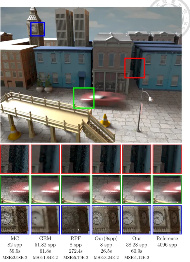
MC GEM RPF Our(8spp) Our Reference 82 spp 51.82 spp 8 spp 8 spp 38.28 spp 4096 spp

59.9s 61.8s 272.4s 26.5s 60.9s

Figure 5.4: Comparisons on the TOWN scene with an environment light, an area light, and heavy occlusion. The image on the top is our result. GEM fails to adapt to textures, and RPF does not obtain enough samples to reconstruct the scene within the given time. Also, RPF contains heavy noise due to its sampling bilateral ﬁltering approach. Our method adaptively samples the dark noisy area and preserves details well.

(35)

MC GEM RPF Our(low spp) Our

Figure 5.5: This ﬁgure visualizes the per-pixel relative error of each method. Scenes from the top: SIBENIK, TEAPOT, SPONZA, TOWN. The images show that overall our method produces lower error compare to other methods. It is worth to note that GEM gives lower error in a few regions, such as the shadowed area of the elevated walkway in the TOWN scene, this is because GEM can have more samples under an equal-time comparison, and our feature buﬀer does not capture the edge well in these region. Still, our method produces a much higher quality image overall compare to GEM.

(36)

GEM (MSE:2.87E-4) Our (MSE:3.56E-4)

Figure 5.6: The proposed SURE-based framework incorporated with an isotropic Gaussian ﬁlterbank and compared with GEM [26]. The results and scale selection maps generated by both methods are similar.

(37)

Global cross non-local means SURE cross non-local means

MSE:8.50E-2 MSE:1.2E-2

Global SURE Reference Global SURE Reference

Figure 5.7: Comparison of cross non-local means ﬁlters without and with SURE- based framework. Compared to the global cross non-local means ﬁlter, our SURE- based optimization largely alleviates the oversmoothing problem. The sampling rate of the noisy input image is about 41 samples per pixel.

(38)

Chapter 6 Conclusion and Future Work

We have presented an eﬃcient adaptive sampling and reconstruction algorithm for reducing noise in Monte Carlo rendering by using Stein’s Unbiased Risk Estima- tor (SURE) in the error estimation framework. For reconstruction, the use of SURE enables us to measure the reconstruction quality for arbitrary ﬁlter kernels. It does away with the limitation of using only symmetric kernels imposed by previous work.

This freedom to use non-symmetric kernels significantly improves the effectiveness of the framework. When performing adaptive sampling, SURE can be used to determine the sampling density. Another contribution of this thesis is an efficient and memory-friendly approach to detect noisy geometric features when rendering depth of field and motion blur. As a result, the proposed adaptive sampling and reconstruction method efficiently eliminates MC noise while preserving the vivid details of a scene. Experiments show the proposed method offers significant improvement over state-of-the-art approaches.

One possible future direction is to implement the proposed algorithms on GPUs for interactive applications. Another possibility is to investigate some recent fast and advanced ﬁlters such as the one proposed by Gastal et al. [12]. We also would like to extend the SURE-based framework to animation rendering. In the current algorithm, as there is no built-in mechanism speciﬁcally designed for temporal data, temporal coherence cannot be guaranteed. In practice, we have experimented with a naive approach that renders each frame independently. The results look good enough

(39)

with only very subtle temporal ﬂicking. However, a better way to handle animation would be to consider temporal samples and perform ﬁltering in the spatial-temporal domain. Finally, it would also be interesting to adapt SURE to other rendering applications that require error estimation.

(40)

Bibliography

[1] K. Bala, B. Walter, and D. P. Greenberg. Combining edges and points for interactive high-quality rendering. ACM Trans. Graph. (Proceedings of SIGGRAPH 2003), 22(3):631–640, 2003.

[2] P. Bauszat, M. Eisemann, and M. Magnor. Guided image ﬁltering for interactive high-quality global illumination. Computer Graphics Forum (Proceedings of EGSR 2011), 30(4):1361–1368, 2011.

[3] L. Belcour, C. Soler, K. Subr, N. Holzschuch, and F. Durand. 5D Covariance Tracing for Eﬃcient Defocus and Motion Blur. 2013.

[4] T. Blu and F. Luisier. The SURE-LET approach to image denoising. IEEE Transactions on Image Processing, 16(11):2778–2786, 2007.

[5] A. Buades, B. Coll, and J.-M. Morel. A non-local algorithm for image denoising.

In Proceedings of IEEE Computer Vision and Pattern Recognition (CVPR 2005), pages 60–65, 2005.

[6] J. Chen, B. Wang, Y. Wang, R. S. Overbeck, J.-H. Yong, and W. Wang. Ef- ﬁcient depth-of-ﬁeld rendering with adaptive sampling and multiscale reconstruction. Computer Graphics Forum, 30(6):1667–1680, 2011.

[7] H. Dammertz, D. Sewtz, J. Hanika, and H. P. A. Lensch. Edge-avoiding Á- Trous wavelet transform for fast global illumination ﬁltering. In Proceedings of the Conference on High Performance Graphics (HPG 2010), pages 67–75, 2010.

(41)

[8] D. Donoho and I. M. Johnstone. Adapting to unknown smoothness via wavelet shrinkage. Journal of the American Statistical Association, 90:1200–1224, 1995.

[9] K. Egan, F. Hecht, F. Durand, and R. Ramamoorthi. Frequency analysis and sheared ﬁltering for shadow light ﬁelds of complex occluders. ACM Trans.

Graph., 30(2):Article 9, 2011.

[10] K. Egan, Y.-T. Tseng, N. Holzschuch, F. Durand, and R. Ramamoorthi. Fre- quency analysis and sheared reconstruction for rendering motion blur. ACM Trans. Graph. (Proceedings of SIGGRAPH 2009), 28(3):Article 93, 2009.

[11] C. V. Fiorio. Conﬁdence intervals for kernel density estimation. Stata Journal, 4(2):168–179, 2004.

[12] E. S. L. Gastal and M. M. Oliveira. Adaptive manifolds for real-time high- dimensional ﬁltering. ACM Trans. Graph. (Proceedings of SIGGRAPH 2012), 31(4):Article 33, 2012.

[13] T. Hachisuka, W. Jarosz, and H. W. Jensen. A progressive error estimation framework for photon density estimation. ACM Trans. Graph. (Proceedings of SIGGRAPH Asia 2010), 29(6):Article 144, 2010.

[14] T. Hachisuka, W. Jarosz, R. P. Weistroﬀer, K. Dale, G. Humphreys, M. Zwicker, and H. W. Jensen. Multidimensional adaptive sampling and reconstruction for ray tracing. ACM Trans. Graph. (Proceedings of SIGGRAPH 2008), 27(3):Article 33, 2008.

[15] J. Lehtinen, T. Aila, J. Chen, S. Laine, and F. Durand. Temporal light ﬁeld reconstruction for rendering distribution eﬀects. ACM Trans. Graph. (Proceed- ings of SIGGRAPH 2011), 30(4):Article 55, 2011.

[16] J. Lehtinen, T. Aila, S. Laine, and F. Durand. Reconstructing the indirect light ﬁeld for global illumination. ACM Trans. Graph. (Proceedings of SIGGRAPH 2012), 31(4):Article 51, 2012.

(42)

[17] P. C. Mahalanobis. On the generalized distance in statistics. In Proceedings of the National Institute of Science of India, volume 2, pages 49–55.

[18] S. U. Mehta, B. Wang, and R. Ramamoorthi. Axis-aligned ﬁltering for interactive sampled soft shadows. ACM Trans. Graph. (Proceedings of SIGGRAPH Asia 2013), 31(6):Article 163, 2012.

[19] S. U. Mehta, B. Wang, R. Ramamoorthi, and F. Durand. Axis-aligned ﬁltering for interactive physically-based diﬀuse indirect lighting. ACM Trans. Graph.

(Proceedings of SIGGRAPH 2013), 32(4), 2013.

[20] D. P. Mitchell. Generating antialiased images at low sampling densities. In Proceedings of SIGGRAPH 1987, pages 65–72, 1987.

[21] D. P. Mitchell. Spectrally optimal sampling for distribution ray tracing. In Proceedings of SIGGRAPH 1991, pages 157–164, 1991.

[22] B. Moon, J. Y. Jun, J. Lee, K. Kim, T. Hachisuka, and S.-E. Yoon. Robust image denoising using a virtual ﬂash image for monte carlo ray tracing. Comput.

Graph. Forum, 32(1):139–151, 2013.

[23] R. S. Overbeck, C. Donner, and R. Ramamoorthi. Adaptive wavelet rendering.

ACM Trans. Graph. (Proceedings of SIGGRAPH Asia 2009), 28(5):Article 140, 2009.

[24] M. Pharr and G. Humphreys. Physically Based Rendering: From Theory To Implementation. Morgan Kaufmann Publishers Inc., 2nd edition, 2010.

[25] T. Qiu, A. Wang, N. Yu, and A. Song. Llsure: Local linear sure-based edge-preserving image ﬁltering. IEEE Transactions on Image Processing, 22(1):80–90, 2013.

[26] F. Rousselle, C. Knaus, and M. Zwicker. Adaptive sampling and reconstruction using greedy error minimization. ACM Trans. Graph. (Proceedings of SIGGRAPH Asia 2011), 30(6):Article 159, 2011.

(43)

[27] B. Segovia, J. C. Iehl, R. Mitanchey, and B. Péroche. Non-interleaved deferred shading of interleaved sample patterns. In Proceedings of the 21st ACM SIG- GRAPH/EUROGRAPHICS Symposium on Graphics Hardware, pages 53–60, 2006.

[28] P. Sen and S. Darabi. On ﬁltering the noise from the random parameters in Monte Carlo rendering. ACM Trans. Graph., 31(3):Article 18, 2012.

[29] P. Shirley, T. Aila, J. Cohen, E. Enderton, S. Laine, D. Luebke, and M. McGuire. A local image reconstruction algorithm for stochastic rendering. In Proceedings of Symposium on Interactive 3D Graphics and Games, pages 9–14, 2011.

[30] C. Soler, K. Subr, F. Durand, N. Holzschuch, and F. Sillion. Fourier depth of ﬁeld. ACM Trans. Graph., 28(2):Article 18, 2009.

[31] C. M. Stein. Estimation of the mean of a multivariate normal distribution.

Annals of Statistics, 9(6):1135–1151, 1981.

[32] R. Tamstorf and H. W. Jensen. Adaptive sampling and bias estimation in path tracing. In Proceedings of Eurographics Rendering Workshop, pages 285–295, 1997.

[33] D. Van De Ville and M. Kocher. SURE-based non-local means. IEEE Signal Processing Letters, 16(11):973–976, 2009.

[34] R. Xu and S. N. Pattanaik. A novel Monte Carlo noise reduction operator.

IEEE Computer Graphics and Applications, 25(2):31–35, 2005.

(44)

Appendix A

Derivatives for ﬁlters

To compute SURE for reconstruction filters, we must calculate their derivatives dF (ci)/dci and substitute into Equation 3.2. For the cross bilateral filter, from Equation 4.2, we have (note that w_ii= 1 according to the definition in Equation 4.1)

F (c_i) =

∑_n

j=1w_ijc_j

∑_n

j=1w_ij =

∑

j̸=iw_ijc_j + c_i

∑_n

j=1w_ij . (A.1)

Let W_i =∑_n

j=1w_ij. After applying the quotient rule of derivatives, we have dF (c_i)

dci

= (^d(

∑

j̸=iwijcj+1)

dci )−^dW_dc_iⁱF (c_i) Wi

. (A.2)

After substituting ^dw_dc^ij

i = ^(c^j_σ^−c2ⁱ⁾

r w_ij into Equation A.2, and after some manipulations, we obtain

dF (c_i) dc_i = 1

W_i + 1

σ²_r(F²(c_i)− F (ci)²), (A.3) where

F²(c_i) =

∑n

j=1w_ijc_j²

∑n j=1wij

.

For the cross non-local means ﬁlter, its dF (c_i)/dc_i is dF (c_i)

dc_i = 1

W_i + 1

|N|σr²

(F²(c_i)− F (ci)²)+

1

|N|σr²Wi

∑

n∈N

w_i,i_−n(c_i − ci+n)(F (c_i)− ci−n),

(A.4)

(45)

where W_iand F²(c_i) are deﬁned similarly as above. Similar derivations can be found in Van De Ville and Kocher’s paper [33].