國立臺灣大學電機資訊學院資訊工程學系 碩士論文
Department of Computer Science and Information Engineering College of Electrical Engineering and Computer Science
National Taiwan University Master Thesis
有效使用記憶體的小盤面圍棋求解演算法及實作 Memory efficient algorithms and implementations for
solving small-board-sized Go
林弘承
Hung-Cheng Lin
指導教授:薛智文教授 Advisor: Chih-Wen Hsueh, Ph.D.
共同指導教授:徐讚昇教授 Co-Advisor: Tsan-sheng Hsu, Ph.D.
中華民國 107 年 8 月 August, 2018
Acknowledgements
The author thanks his advisor, Prof. Tsan-sheng Hsu, and his co-advisor, Prof. Chih-Wen Hsueh, for their continuous support for his graduate study and research and for their patience and the motivation and knowledge that they have given. The thesis would not have been completed without their help.
The author would also like to thank his colleague, Cheng Yueh, for his insightful thoughts during discussions.
The author would also like to thank the members of his family for their support throughout his life.
摘要
之前的研究已有弱解的小盤面圍棋解法,在此基礎上,我們希望能 找到小盤面圍棋的強解,做為更深入的分析。我們應用圍棋的特性來 壓縮狀態的儲存空間,並用回溯分析以找出所有可能狀態的最佳解,
也設計出一個儲存於硬碟的資料庫以供後續存取。為了儲存及更新大 量的狀態,使用壓縮後並儲存分割的資料區塊於記憶體而非硬碟,在 需要使用的時候再解壓,可達到速度和記憶體用量的平衡。此方法亦 可應用於巨量資料的處理。此外,我們由結果觀察並證明正確一路圍 棋的最佳簡單著手規則。
關鍵字: 小盤面圍棋, 狀態空間搜尋, 回溯分析, 記憶體內運算
Abstract
Previously studies have weakly solved the problem of playing small-board- sized Go, but this study determines a strongly-solved solution and a database to access afterward.
State reduction is applied by the features of Go; and then retrograde anal- ysis is used to find the optimal answer of every possible state of small-board- sized Go.
Dealing with large state information, an in-memory method is used to search the states for small-board-sized Go. Saving separated compressed data in the memory, instead of on a disk, and decompressing this data on demand, to balance performance and memory usage, in order to solve the problem efficiently. This method can also be applied to large scale data processing.
A method is also determined that obtains the optimal result for boards with a single row.
Keywords: Small-board-Go, State Space Search, Retrograde Analysis, In- Memory Computing
Contents
Acknowledgements iii
摘要 v
Abstract vii
1 Motivation 1
2 Related Work 3
2.1 Previous Works . . . 3
2.2 Retrograde Analysis . . . 4
2.3 4× 4 Problems . . . . 5
3 Problem Definition 7 3.1 The Rules of Go . . . 7
3.1.1 Basic Rules . . . 7
3.1.2 Rules of Ko . . . 8
3.1.3 Scoring Rules . . . 9
3.2 Seki . . . 10
3.3 The Rules that are used for this study . . . 10
3.4 Goal . . . 11
4 Method 13 4.1 Encoding of States . . . 13
4.2 Legal States and Reduction . . . 15
4.2.1 Terminal States . . . 15
4.2.2 State Reduction . . . 16
4.2.3 Sort Order . . . 16
4.3 Search Algorithm . . . 18
4.3.1 Preprocessing . . . 19
4.3.2 Algorithm to Search the Game Result . . . 19
4.3.3 Algorithm to Find the Score . . . 21
4.3.4 Data Structure used to save the Search Result . . . 21
4.3.5 Validation . . . 24
4.3.6 Misc . . . 25
4.4 In-Memory Method . . . 25
4.5 Memory Issues . . . 26
4.6 Performance Issues . . . 26
5 Result 29 5.1 Configuration . . . 29
5.2 Experimental Results . . . 30
5.3 Performance Considerations . . . 30
5.3.1 Memory Block Size and Memory Chunk Size . . . 30
5.3.2 Sort Order . . . 32
5.3.3 Number of Edges . . . 33
5.3.4 Search Depth . . . 33
5.3.5 Data Saving Method . . . 36
5.4 Variation: Circular Board . . . 37
5.5 Properties of Go . . . 38
5.5.1 Seki . . . 38
5.5.2 Strongly Connected Component . . . 38
5.6 Strategy for 1× n Go . . . 41
5.6.1 Step(s) = 1 . . . . 44
5.6.2 Step(s) = 3 . . . . 44
5.6.3 Step(s) = 2 . . . . 45
5.6.4 Conclusion . . . 49
6 Conclusion and Future Work 53 6.1 Conclusion . . . 53
6.2 Future Work . . . 54
6.2.1 Rule-Based 2× N Go . . . 54
6.2.2 Other Sorting Criteria . . . 54
References 55
List of Figures
1.1 Fair opening examples of 4× 4 Go board . . . . 1
2.1 4× 4 problem 1 . . . . 5
2.2 4× 4 problem 2 . . . . 5
3.1 Basic rules of Go . . . 8
3.2 Different results when applying different scoring rules . . . 9
3.3 An example of Seki . . . 10
4.1 A 5× 5 state reduction example, the triangle symbol is Ko move . . . 15
4.2 A terminal state example. Black has no legal move, so white can simply pass to win the game. . . 16
4.3 First 10 states of 4× 4 board in serial order . . . 17
4.4 First 10 states of 4× 4 board in piece order . . . 18
4.5 Using increasing order of score to update cause wrong result. . . 22
4.6 Memory usage of state array using memory block and memory chunk . . 25
5.1 Correlation between time and edge count . . . 33
5.2 Time distribution of search depth in different size of Go boards . . . 34
5.3 Time distribution of search depth in different size of Black-non-fully-win Go boards . . . 34
5.4 Time distribution of search depth in different size of Black-fully-win Go boards . . . 35
5.5 Comparison of zlib and I/O performance in different memory block size. . 37
5.6 Three board positions can be compressed to one in circular board . . . 37
5.7 Seki example in 4× 4 Go board . . . 39
5.8 cycle example 1: superKo . . . 39
5.9 cycle example 2: states in SCC . . . 40
5.10 Position can be count from another side. . . 41
5.11 An example of White’s Move-Generating Rule . . . 42
5.12 State that apply step 3 and it’s variations . . . 45
5.13 Black plays at position 1 which capture multiple stones . . . 46
5.14 Black plays at position 1 and capture only one stone . . . 47
5.15 More than two strings from position 2 to k − 1. In this example, black string start from position 3 has no liberty . . . 47
5.16 m = k− 1 . . . 50
5.17 m = k + 1 . . . . 51
List of Tables
2.1 Legal State Count for square board Go . . . 4
4.1 List of features and used bits in 5× 5 board state . . . 14
4.2 Encoding of state in Figure 4.1(a) . . . 14
4.3 Encoding of state in Figure 4.1(b) . . . 14
4.4 State statistics of 4× 5 board . . . 17
5.1 List of machines used for the experiment . . . 29
5.2 Result of small-board-sized Go, result B + n means Black win n stones, best move is the coordinate label on the board . . . 31
5.3 Performance and memory usage with different memory size used . . . 32
5.4 Performance in different memory block size with the same memory used . 32 5.5 Influence of sort locality and performance by applying piece order . . . . 32
5.6 Average I/O and zlib performance by testing 13 different memory blocks which is 5× 5 . . . 36
5.7 Average zlib performance with different compression levels in 5× 5 Go. 36 5.8 Result of small-board-sized circular Go board . . . 38
Chapter 1 Motivation
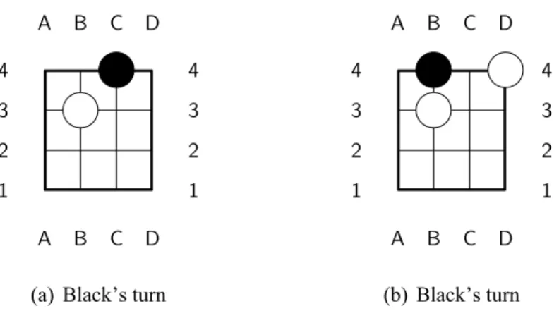
This study determines all possible states for a small rectangular Go board. It is treated as a sub problem of a 9×9 Go or 19×19 Go board, so the search method for small boards may be applied to larger boards. In addition, the fair Komi and opening (see Figure1.1) are determined by solving the small-board-sized Go problem, the optimal result of fair opening is the draw. It is a better way to study the strategy and properties for small-board- sized Go, and may extend to bigger board. By solving small-board-sized Go, we can find the relation between boundary and intersections, which is the important feature of Go.
In order to solve all possible states for small-board-sized Go, a great number of state information is needed to be accessed. A memory-efficient method with acceptable per- formance is required to solve this task.
A A
B B
C C
D D
1 1
2 2
3 3
4 4
(a) Black’s turn
A A
B B
C C
D D
1 1
2 2
3 3
4 4
(b) Black’s turn
Figure 1.1: Fair opening examples of 4× 4 Go board
Chapter 2
Related Work
2.1 Previous Works
Small boards are used for beginners to learn Go. Because 19 × 19 Go requires a long search time, many studies address a smaller Go board and extend the result to larger boards.
Using an Alpha-Beta search with optimization, the problem can be weakly solved for a small rectangular board with less than 30 intersections. For example, the optimal game result and the optimal first move are found in 5× 5, the optimal first move is the center of the board (C3 as Go board coordinate) and the optimal game result is Black fully win (25 points) [1, 2].
Using Meta-MonteCarlo-Tree-Search to build a huge opening book for 7×7 Go, and defeat professional Go players [3].
The variation in a game of Go is a challenge, such as atari-Go and kill-all Go. In atari- Go, the winner is the player that first captures the stone(s), and playing pass is prohibited.
The 5× 5 atari-Go game result is determined as Black’s win [4].
Other studies use a proof-number search to determine the result for specific 7 × 7 kill-all Go opening positions [5]. In kill-all Go, Black plays two stones first, and White wins if there’s a white live string, Black wins if there’s no legal move for both players.
The number of legal states for square Go boards are calculated for size up to 17× 17 and give the boundary of the legal state count for 19× 19 Go [6], the result is shown in
Table 2.1.
Board Size Digit Legal State Number
1 1 1
2 2 57
3 5 12675
4 8 24318165
5 12 414295148741 6 17 62567386502084877
7 23 83677847847984287628595
8 30 990966953618170260281935463385
9 39 103919148791293834318983090438798793469
10 47 96498428501909654589630887978835098088148177857
11 57 793474866816582266820936671790189132321673383112185151899 12 68 577742584895132389982379703074839993272872107569911896559426
51331169
13 80 372497923076863964422949047670245176742491579482087175332547 99550970595875237705
14 93 212667732900366224249789357650440598098805861083269127196623 872213228196352455447575029701325
15 107 107514643083613831187684137548661238097337888203278444027646 01662870883601711298309339239868998337801509491
16 121 481306696382275541642905602248429964648687410096724926394471 959997560745985050222203959114933143180552465546745306704237 7
17 137 190793889196281992046057261818504652201510583381479222439672 692319440591872147679971059923417352092306672884621790900736 59712583262087437
Table 2.1: Legal State Count for square board Go
2.2 Retrograde Analysis
Retrograde analysis is widely used for searching endgames in chess-like game pro- gramming [7], such as Chinese chess [8] and shogi [9]. This method can be also applied to solve the full games when the state-space complexity of the game is small, like awari [10].
Previous study use this method to analyze patterns in Go [11].
[12] categorizes four major regretrograde analysis algorithms by their implementa- tions. Our study use the fourth method, which is the refined method to implement the retrograde analysis algorithm.
2.3 4 × 4 Problems
These 4× 4 problems and solutions are from [13], as shown at Figure 2.1 and Figure 2.2, which is for beginners to learn Go.
A A
B B
C C
D D
1 1
2 2
3 3
4 4
(a) Initial state, black’s turn
A A
B B
C C
D D
1 1
2 2
3 3
4 4
3 1 2
(b) Answer
Figure 2.1: 4× 4 problem 1
A A
B B
C C
D D
1 1
2 2
3 3
4 4
(a) Initial state, black’s turn
A A
B B
C C
D D
1 1
2 2
3 3
4 4
1 2 3
4 5 6
7 8
(b) Answer move 1 to 8
A A
B B
C C
D D
1 1
2 2
3 3
4 4
9 10
11 12
13 14 15
16 17
18 19
(c) Answer move 9 to 19
Figure 2.2: 4× 4 problem 2
Chapter 3
Problem Definition
3.1 The Rules of Go
Go is an ancient game that originated in China. Black and white stones are used to secure territory on the board and to surround the opponent. The basic rules are shown in Figure 3.1.
3.1.1 Basic Rules
Initially, the board is empty and there are vertical and horizontal lines. Each player places black or white stones at the intersections of these lines.
We look the connected set of stones in the same color as a string. The liberty of a string is the number of connected empty intersections. There are many different Go rules, mainly different between rules of Ko and scoring.
We look the connected set of stones in the same color as a string. The liberty of a string is the number of connected empty intersections.
There are many different Go rules, mainly different between rules of Ko and scoring rules.
1. The black player plays first.
2. Black and white players place stones with the corresponding color in order.
3. If the opponent’s string is out of liberty, it is captured and moved off the board.
4. A player cannot play a Ko move.
5. A player cannot play a suicidal move, which is the move that makes his or her string liberty become 0, unless this move involves the capture of an opponent’s string.
6. A player can pass a move. If two players pass continuously, the game is ended and the score is calculated.
Figure 3.1: Basic rules of Go
3.1.2 Rules of Ko
Ko is the rule that prevents a loop in the game. The some commonly used Ko rules are [14] :
1. Basic Ko
2. Positional Superko 3. Situational Superko
Define the board position to be the positions of stones on the board; and the board configuration to be the board position and player’s turn.
Basic Ko
Basic Ko only forbids a move that recreates the position from two moves before, but allows a longer cycle.
Positional Superko
Positional superko prevents the repeat of a board position.
Situational Superko
Situational superko does not allow a play that repeats a board’s configuration.
The rules that are used in professional games are a variant of these three Ko rules.
3.1.3 Scoring Rules
The two main scoring methods involve area scoring and territory scoring [15].
Area Scoring
The player’s score is the number of empty intersections only his color surround and the number of its stones on the board. Area scoring is used in Chinese rules. It’s easier rule to implement in computer Go.
Territory Scoring
Dead stones and stones that are captured are looked as another color’s player’s pris- oners.
The player’s score is calculated in terms of his or her territory and the number of prisoners. Territory is the empty intersections that are controlled by one color. Its detailed definition is different for each set of rules. Territory scoring is used in Japanese rule and Korean rule.
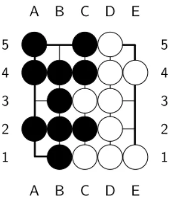
In general, area scoring and territory scoring give the same result or one or two points difference. For example, in Figure 3.2, if there’s no stone captured in the game, the result of territory scoring is draw (Black 3 points, White 3 points), and the result of area scoring is Black win one point (Black 13 points, White 12 points).
A A
B B
C C
D D
E E
1 1
2 2
3 3
4 4
5 5
End of the game
Figure 3.2: Different results when applying different scoring rules
3.2 Seki
Seki is a special case for the scoring rule for Go. It literally means mutual life. Two player’s strings share liberties, if one player fills the liberty, his or her string is captured by another player. However, these strings are alive if they do not occupy the shared liberties.
An example is shown at Figure 3.3. Some rules do not count the score for strings which are Seki [16].
A A
B B
C C
1 1
2 2
3 3
Figure 3.3: An example of Seki
3.3 The Rules that are used for this study
This study uses basic Ko and area scoring without komi. Because komi is not used, the white player does not get compensation when he or she scores.
The basic Ko rule states that when the game falls into a loop, the result of the game is considered to be draw.
It is worthy of note that the Benson algorithm [17] is not used to check dead strings because it only affects the result for unfinished boards, so both players pass when one of the players makes a legal move that does not fill his or her eye. Dead stones are considered to be alive if the opponent does not capture them before game ends.
In summary, the rules that this study uses allow superko and loops whose lengths are longer than 2, stones that seem dead are considered to be alive and the stones in Seki are also included in the score.
3.4 Goal
This study solves the game result (which player wins the game) and the score (the difference in points between the winner and the loser) for all possible states on a small- board-sized Go. These are strongly solved for small-board-sized Go using the criteria for solving two-player zero-sum games with perfect information [18].
Chapter 4 Method
4.1 Encoding of States
Go’s state includes the information about a stone’s position, the Ko position, the pass count and the turn. The degree, the game result and the score are required for the search process.
Let the number of rows on the board be R and the number of columns on the board be C. Ternary representation is sued to map intersections on the board. If an intersection is empty, it is assigned a value of 0 and a black stone and a white stone are respectively assigned values of 1 and 2, so the range of board position values is from 0 to 3R×C.
The Ko position can be represented using a simple position index. Including the situation where there is no Ko, there are R× C + 1 different Ko positions. The pass count includes 0, 1 and 2. The turn indicates the player that can play a move in the current state.
In this implementation, it is reduced (See Section 4.2).
Ko and pass can be combined to reduce the number of bits that are used. When the pass is 1 or 2, there is definitely no Ko, so Ko and the pass have R× C + 3 different combinations.
The degree (the number of legal next states), the game result and the score are saved and all information is encoded into a bit array, to reduce the amount of memory that is used.
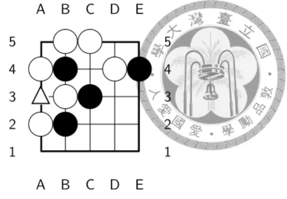
The 5× 5 board that shown at Figure 4.1(a) can be encoded to Table 4.2.
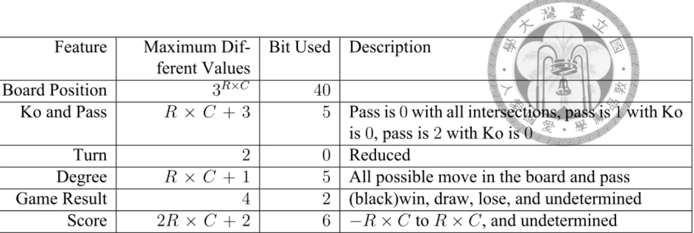
Feature Maximum Dif- ferent Values
Bit Used Description
Board Position 3R×C 40
Ko and Pass R × C + 3 5 Pass is 0 with all intersections, pass is 1 with Ko is 0, pass is 2 with Ko is 0
Turn 2 0 Reduced
Degree R × C + 1 5 All possible move in the board and pass Game Result 4 2 (black)win, draw, lose, and undetermined
Score 2R × C + 2 6 −R × C to R × C, and undetermined Table 4.1: List of features and used bits in 5× 5 board state
Feature Value Binary Representation Description
Board Position 4091124856 100111000011001101 01101110111000010
00020000100020102121010103
Ko and Pass 3 00011 Ko at position 3, pass is 0
Degree 13 01101 Empty intersections with-
out position 1 and Ko
Game Result 3 11 Undetermined
Score 51 110011 Undetermined, 2× R × C + 1 = 51
Table 4.2: Encoding of state in Figure 4.1(a)
Feature Value Binary Representation Description
Board Position 72664314 10001010100110
0010011111010
00000000120012012012002203
Ko and Pass 11 01011 Ko at position 11, pass is 0
Degree 13 01101 Doesn’t change after reduction
Game Result 3 11 Doesn’t change after reduction
Score 51 110011 Doesn’t change after reduction
Table 4.3: Encoding of state in Figure 4.1(b)
A A
B B
C C
D D
E E
1 1
2 2
3 3
4 4
5 5
White’s turn
(a) A 5× 5 state without reduction
A A
B B
C C
D D
E E
1 1
2 2
3 3
4 4
5 5
Black’s turn
(b) A 5× 5 state with reduction
Figure 4.1: A 5× 5 state reduction example, the triangle symbol is Ko move
A 5× 5 board uses 58 bits per state. Because the memory must be aligned, 64 bits are used for each state.
4.2 Legal States and Reduction
Only legal states are searched, which are the states that follow the rules. Illegal states, such as a string with no liberty or an impossible Ko position, are discarded in the preprocessing phase.
4.2.1 Terminal States
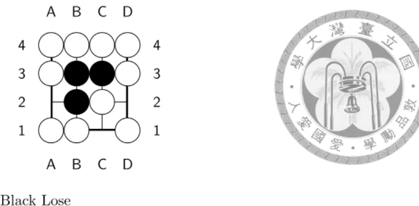
Terminal states are the set of states that can directly determine the result of the game without processing, such as a state whereby one player cannot make any legal move and the other player is currently winning (see Figure 4.2). A move is legal when the position of the move has an empty intersection that can be occupied by the player’s stone without breaking the rules.
Terminal states are not saved in the memory because the result can be calculated when it is needed.
Obviously, all states for which pass is 2 are terminal states.
A A
B B
C C
D D
1 1
2 2
3 3
4 4
Black Lose
Figure 4.2: A terminal state example. Black has no legal move, so white can simply pass to win the game.
4.2.2 State Reduction
States with symmetrical board configuration have the same result and score. Thus, these states can be reduced into one state.
The state that has the lowest value for symmetrical board positions is specified as the reduced state. There are at most 8 different square board states that are considered to be the same state. For a rectangular board, there are at most 4 different states that can be reduced into one.
The Ko position can also be reduced by specifying the lowest index for Ko positions in all symmetrical Ko positions.
Turn is reduced by changing the turn and the color of the stones on the board together.
The states are reduced to black’s turn, so it is not necessary to include turn information in the reduced state.
Figure 4.1 is an example of state reduction.
We keep all the states reduced during the search phase. In this way, the number of states that as shown in Table 4.4 must be searched is also reduced.
4.2.3 Sort Order
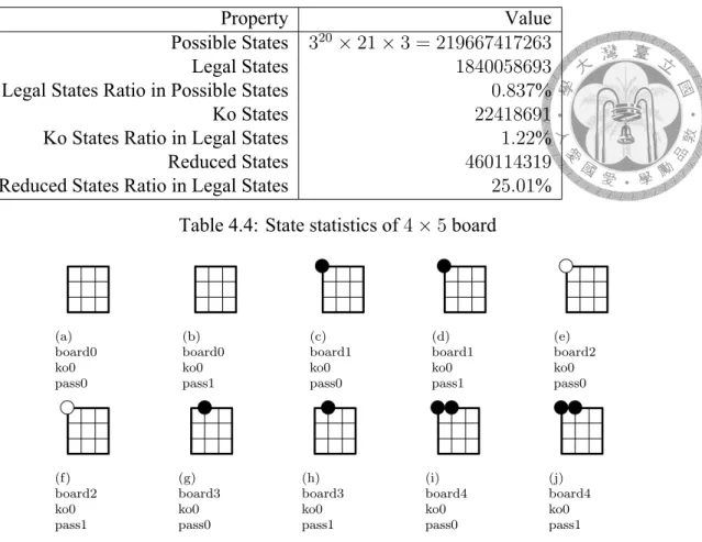
Serial Order
The states are sorted in terms of features in the order: board position > Ko position
> pass count. An example is shown in Figure 4.3.
Property Value Possible States 320× 21 × 3 = 219667417263
Legal States 1840058693
Legal States Ratio in Possible States 0.837%
Ko States 22418691
Ko States Ratio in Legal States 1.22%
Reduced States 460114319
Reduced States Ratio in Legal States 25.01%
Table 4.4: State statistics of 4× 5 board
(a) board0 ko0 pass0
(b) board0 ko0 pass1
(c) board1 ko0 pass0
(d) board1 ko0 pass1
(e) board2 ko0 pass0
(f) board2 ko0 pass1
(g) board3 ko0 pass0
(h) board3 ko0 pass1
(i) board4 ko0 pass0
(j) board4 ko0 pass1
Figure 4.3: First 10 states of 4× 4 board in serial order
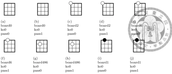
Piece Order
Another sorting method is used to obtain a better locality in performing sorting.
Sorting using the order: total number of stones on the board > number of black stones on the board > board position > Ko position > pass count. An example is shown in Figure 4.4.
The former sorting method is called “serial order” and the latter sorting method is called “piece order”.
Let Stotaland Sblackbe the total number of stones and the total number of black stones for the current states. The total number of stones and the total number of black stones for previous states are Stotal′ and Sblack′ . If there is no previous capture, Stotal′ = Stotal − 1 and Sblack′ = Sblack − 1. Thus, previous states are concentrated into a smaller range in state array. By using piece order, the frequency of a memory block being compressed and decompressed is then decreased. Details will be described in Section 4.4.
(a) board0 ko0 pass0
(b) board0 ko0 pass1
(c) board2 ko0 pass0
(d) board2 ko0 pass1
(e) board6 ko0 pass0
(f) board6 ko0 pass1
(g) board486 ko0 pass0
(h) board486 ko0 pass1
(i) board1 ko0 pass0
(j) board1 ko0 pass1
Figure 4.4: First 10 states of 4× 4 board in piece order
4.3 Search Algorithm
Algorithm 1 states the main processes for the algorithm to solve small-board-sized Go.
Algorithm 1: Main Processes of Search Algorithm
1 Function Main():
2 Preprocessing() // Section 4.3.1
3 SearchGameResult() // Section 4.3.2
4 SearchScore() // Section 4.3.3
5 SaveSearchResult() // Section 4.3.4
6 Validation() // Section 4.3.5
Preprocessing is required before the search and the process is described in Section 4.3.1. The search game result involves searching the game results for all legal states, as described in Section 4.3.2. The search score involves searching the score for all legal states, as described in Section 4.3.3. The search result is saved by saving the game result and the score into the database, as described in Section 4.3.4. Validation is an optional process that verifies that the result is correct and is described in Section 4.3.5.
4.3.1 Preprocessing
The legal states are calculated, sorted and saved in the preprocessed files. The data can be directly dumped into the memory as an array.
4.3.2 Algorithm to Search the Game Result
Concept
The main concepts of the search result algorithm are:
1. Let S be the state with undetermined result 2. Let S′be the state that supersedes S
3. If there exists a state for which the result is lose in S′, the result for S is a win 4. If for all states in S′, the result is a win, the result for S is a loss
5. Repeat steps 1 to 4 until there is no undetermined state that can be updated as win or lose
6. The remaining undetermined states are considered to be draws
If there is an undetermined state S, such that the result for its next states has at least one undetermined state S′and has no loss state, then S′is the optimal next state. Because S′ is also an undetermined state, there is also an undetermined state S′′in the next states of S′, so the game does not end and the result is draw.
Retrograde Analysis Algorithm
Let Wi be the states that wins in i moves, Li be the states that loses in i moves.
The fourth method in [12], which is called “Layered Backward Propagation with Unknown-children counting”, is used to categorize the states in terms of the game result and the depth of the search, and the result is propagated to the previous states, as Wi→Li+1, and Li→Wi+1.
In this algorithm, every possible state propagates its value only once. When the result is a loss, it is necessary to check that all of its next states are wins, so information about undetermined next states is retained to determine whether the state is a loss.
The detailed algorithm is shown in Algorithm 2.
Algorithm 2: Retrograde Analysis Search Result Algorithm
/* Wi is the set of states that will win in i turn */
/* Li is the set of states that will lose in i turn */
1 W0 ← terminal states that result is win
2 L0 ← terminal states that result is lose
3 i← 0
4 while Wi ̸= ϕ or Li ̸= ϕ do
5 S ← Wi
6 S′ ← findP reviousStates(S)
7 sort S′
8 foreach State s∈ S do
9 if s.result̸= undetermined then
10 S.remove(s)
11 remove duplicate states in S
12 foreach State s∈ S do
13 s.result← lose
14 Li+1← S
15
16 S ← Li
17 S′ ← findP reviousStates(S)
18 sort S′
19 foreach State s∈ S do
20 if s.result̸= undetermined then
21 S.remove(s)
22 count the number of duplicate states in S
23 foreach State s∈ S do
24 s.degree← s.degree - count of s in S
25 if s.degree = 0 then
26 s.result← win
27 add s into Wi+1
28 foreach State s∈ Sarrdo
29 if s.result = undetermined then
30 s.result← draw
Determining previous States
P reviousState is the class that stores the intermediate data structure. This is tem- porarily saved in a cache in order to determine actual states. One P reviousState can represent multiple legal states that have the same board position, but a different Ko or
pass.
Algorithm 3: Find Previous States
1 Function findPreviousStates(State s):
2 if s has Ko then
3 similar to the part of s.pass = 0, but check previous states can generate Ko
4 else if s.pass = 0 then
5 foreach white stone w ∈ s do
6 find possible captured strings from 4 directions
7 foreach combination c∈ possible capture strings combination do
8 previousBoard← s.board + captured strings in c − w
9 append previousBoard to possibleBoardSet
10 return (PreviousState(possibleBoard, pass = 0 or 1)) for each possibleBoard∈ possibleBoardSet
11 else if s.pass = 1 then
12 return PreviousState(s, pass = 0 or 1)
13 else if s.pass = 2 then
14 s.pass← 1
15 return s
4.3.3 Algorithm to Find the Score
Retrograde analysis is also used to search the score, but a different algorithm is used.
The states for which pass is 2 and which win and lose the most are initially determined.
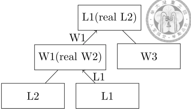
Their score is then propagated to their previous states. This search method is repeated to search for the states in decreasing order of the absolute value of the score. Figure 4.5 shows the wrong result for a search in non-decreasing order of the absolute value of the score.
This method ensures for a state S, all of its next states S′are propagated to S no more than once. This implies that the state does not get a score that is better than its real score during the search phase. The details are shown in Algorithm 4 and Algorithm 5.
4.3.4 Data Structure used to save the Search Result
Because many differently sized boards are saved in the database, not all of the infor- mation is saved in the memory when there is a database query. The state results are saved
L1(real L2)
W1(real W2)
L2 L1
W3 W1
L1
Figure 4.5: Using increasing order of score to update cause wrong result.
Algorithm 4: Search Score Algorithm Input : State array which result is known
Output: State array which result and score is known
1 State queue q
/* from win R× C and lose R × C to win 1 and lose 1 */
2 for score← R × C to 1 do
/* find terminal states which score equals to current score */
3 foreach State s∈ compressedStates do
4 if s.pass = 2 and s.score = score then
5 q.push(s)
6 while q ̸= ϕ do
7 state s← queue.top()
8 q.pop()
9 foreach State ps∈ previous states of s do
10 if updateScore(ps, s.result, s.score) then
// if update success, ps.score = score, so it should also propagate to its previous states
11 q.push(ps)
Algorithm 5: Update Score
Input : State and current score to update Output: Update success or not
1 Function updateScore(State s, int result, int score)
2 if s is already updated then
3 return false
4 if result = lose and s.result = win then
// Because we search from high score to low score and state result is win, so it is the best result, the score of s is determined
5 s.degree← 0
6 else
7 s.degree← s.degree-1
8 if -score > s.score or s.score = undetermined then // update to currently best score
9 setScore(-score)
// degree is 0 means score is found
10 return s.degree = 0
on disk to save time.
The scores for each state’s next states are stored in a file. The result is accessed by specifying the index of the state and then reading the information directly from the file.
Each state has at most (R× C + 1) next states, including pass. Each score is saved using 5 bits (see Section 4.1). Let the number of legal states be N. The size of the result file is 5× N × (R × C + 1) bits.
The following is the process to determine the result for a state.
1. When there is a query, the state is transformed to the reduced state.
2. The index of the state in the state file is then obtained. The state file contains the same data as the legal state array.
3. The result is then accessed from the result file using the index.
For each query of a state, a binary search of the file and random access disk is con- ducted to determine the game result for the state and its next states.
The state file is separated into multiple files, which have the same number of states as the memory blocks, so less time is required for a binary search.
4.3.5 Validation
This is an optional process to check whether the search result is reasonable, as shown in Algorithm 6.
Algorithm 6: Function for validating the result Output: the final result is reasonable or not
1 Function validate():
2 foreach legal state S do
3 S′ ← possible next states of state S
4 flag← false
5 if S.result is draw then
6 foreach state s∈ S′do
7 if s.result is win then
8 return false
9 if s.result is draw then
10 flag← true
11 else if S.result is win then
12 k← S.score
13 foreach state s∈ S′do
14 if s.result is win then
15 if s.score > k then
16 return false
17 if s.score is k then
18 flag← true
19 else if S.result is loss then
20 foreach state s∈ S′do
21 if s.result is win or draw then
22 return false
23 if s.result is loss then
24 if s.score < k then
25 return false
26 if s.score is k then
27 flag← true
28 if flag is false then
29 return false
4.3.6 Misc
The in-memory data is transferred to the disk after each iteration, so the process can be continued if an error occurs.
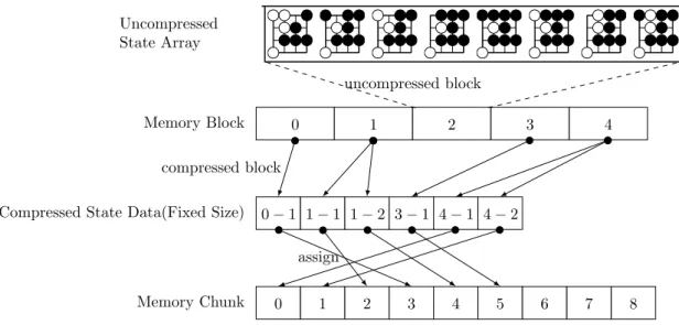
4.4 In-Memory Method
When the size of board increases, the number of legal states increases exponentially.
Thus, the state data cannot all be stored in the memory. Unused states can be temporarily saved to disk, but the I/O operation is time-consuming, so an in-memory method is used for the proposed program.
This study uses zlib [19, 20] library to compress or decompress data in the memory.
The state array is divided into several fixed-sized memory blocks and these blocks are compressed by zlib if they are not in use.
In general, the greater the number of uncompressed memory blocks the better. The number of uncompressed memory blocks depends on the size of the available memory.
Larger memory blocks are used to allow more uncompressed states at a given time.
0 1 2 3 4
0− 1 1 − 1 1 − 2 3 − 1 4 − 1 4 − 2
0 1 2 3 4 5 6 7 8
Memory Block
Compressed State Data(Fixed Size)
Memory Chunk Uncompressed State Array
uncompressed block
compressed block
assign
Figure 4.6: Memory usage of state array using memory block and memory chunk
Data is compressed or decompressed at the level of the memory block and data is saved or read at the level of the memory chunk. The relationship is shown in Figure 4.6.
The algorithm is shown as Algorithm 7.
4.5 Memory Issues
As well as the legal state array, additional information is stored in the memory to accelerate the search process.
A state is represented by its index in the state array. Flags are saved in the memory as Boolean arrays to allow quick access. The information includes the result of whether state has already been searched, or current states in Wi or Li. These Boolean arrays are the same size as the number of legal states. For a 5× 5 Go board, each Boolean array uses 19.59 GB. Directly saving the states into the array requires a maximum of 187 GB, which is too large to save several these data in the memory.
The following are lists of Boolean arrays.
• hasResult: already searched states (Wk, Lk, k < i)
• win: currently searched win states (Wi)
• lose: currently searched lose states (Li)
• newwin: win states to be searched in the next iteration (Wi+1)
• newlose: lose states to search in next iteration (Li+1)
A temporary state array is used as a cache to save states and will be transformed into array indices on batch when the cache is full. The size of cache is flexible, but the larger the cache, the better the performance. In general, the cache must be able to contain at least one uncompressed memory block.
4.6 Performance Issues
State data can be used to find previous states that have Ko, to obtain or to set a result, a score or a degree of a state.
There is a bottleneck because a binary search of the uncompressed memory block is required to obtain the index of a state in the array. If the state is in the compressed memory block, it must be decompressed before it can be used.
When the cache is full, a binary search is used to determine the indices, or a seg- mental scan over the array is needed to determine the index. If the number of states in a memory block is more than log2(state per block), this method is better than the binary search method in terms of time complexity.
Algorithm 7: Memory Related Functions
1 In-memory block index queue q
/* fixed size memory array to read/write, pre-allocated */
2 MemoryChunk array chunks
3 MemoryBlock array blocks
4 State array blockFirstState
/* record first state of each memory blocks */
5 Function decompressBlock(blockindex)
6 if blockindex∈ q then
7 return
8 if number of uncompressed block is up to limit then
9 block lastUsedBlock← blocks[q.front()]
10 q.pop()
11 lastUsedBlock.compress()
12 blocks[blockindex].decompress()
13 q.push(blockindex)
14 Function getStateIndex(State s)
15 blockIndex← blockFirstState.binarySearch(s)
16 if blocks[blockIndex] not uncompressed then
17 decompressBlock(blockIndex)
18 stateIndex← blocks[blockIndex].binarySearch(s)
19 return blockIndex× STATEPERBLOCK + stateIndex
20 Function getState(index)
21 blockIndex← index ÷ STATEPERBLOCK
22 stateIndex← index mod STATEPERBLOCK
23 if blocks[blockIndex] not uncompressed then
24 decompressBlock(blockIndex)
25 return blocks[blockIndex].getState(stateIndex)
26 Function compress()
/* compress a memory block */
27 compressedArray← zlib.compress(stateArray)
28 stateArray.clear()
29 distribute compressArray to multiple memory chunks
30 Function decompress()
/* decompress a memory block */
31 combine memory chunks to form compressedArray
32 clear used memory chunks
33 stateArray← zlib.decompress(compressedArray)
34 compressedArray.clear()
Chapter 5 Result
5.1 Configuration
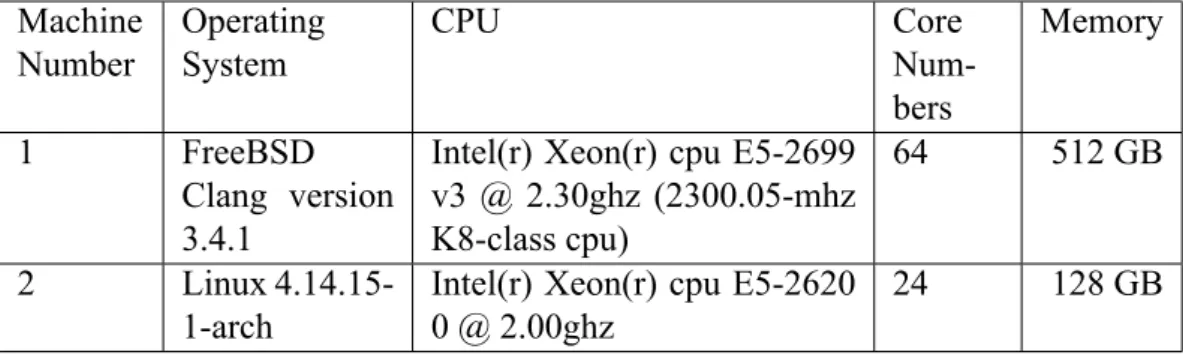
The following experiments were run on FreeBSD Clang version 3.4.1 using cpu In- tel(r) Xeon(r) cpu E5-2699 v3 @ 2.30 ghz (2300.05-mhz K8-class cpu), 64 cores with an available memory of 512 GB. Experiments for smaller boards are run on Linux 4.14.15- 1-arch using cpu Intel(r) Xeon(r) cpu E5-2620 0 @ 2.00ghz, 24cores with an available memory of 128 GB. The former is called Machine 1 and the latter is called Machine 2.
All experiments that were run on Machine 1 are specified and the other experiments were run on Machine 2. Table 5.4 shows the configurations of these two machines.
This study used g++ 8.1.0 as the compiler and zlib 1.2.11 to compress and decompress memory blocks.
Machine Number
Operating System
CPU Core
Num- bers
Memory
1 FreeBSD
Clang version 3.4.1
Intel(r) Xeon(r) cpu E5-2699 v3 @ 2.30ghz (2300.05-mhz K8-class cpu)
64 512 GB
2 Linux 4.14.15-
1-arch
Intel(r) Xeon(r) cpu E5-2620 0 @ 2.00ghz
24 128 GB
Table 5.1: List of machines used for the experiment
5.2 Experimental Results
Define Edge Count to be the sum of the number of the next states for all states. The results for rectangular Go boards are listed in Table 5.2, the biggest size board searched is 2× 11.
The relation between search time and edge count is positive relative. Because we use less ratio of cache in 2× 11, it cost far more time to search.
5.3 Performance Considerations
Experiments were conducted to determine the factors that affect search performance.
5.3.1 Memory Block Size and Memory Chunk Size
The memory block must be neither too small nor too large. If the memory block is too small, the frequency of compression and decompression is increased. If the memory block is too large, the time to compress and decompress is increased.
Because the size of the memory chunk only affects the segmentation of compressed blocks, it has no obvious effect on performance. The results are shown in Table 5.3 and Table 5.4.
In order to optimize the search process, the maximum number of uncompressed states not exceeding the memory limit is first computed and then the best memory block size is decided to minimize the running time.
If the memory block size is larger, the total number of states that must be decom- pressed during an iteration is greater, but there is a greater compression ratio. If the mem- ory block size is smaller, the total number of states that must be decompressed during an iteration is smaller because it is not necessary to access some compressed memory block.
However, we need to use more total memory.
Size Depth Compressed State Number
Edge Count Time Best
Result
Best First Move
1× 1 – – – – draw pass
1× 2 – – – – draw pass
1× 3 – – – – B + 03 B1
1× 4 – – – – B + 04 B1
1×n n ≤ 20 and
n ≥ 5
– – – – draw –
2× 2 2 26 72 0.164 second draw A1
2× 3 11 293 963 0.167 second draw A1,
B1
2× 4 18 2169 8591 0.234 second B + 08 A1,
B1
2× 5 30 18205 84906 0.791 second B + 10 B1,
C1
2× 6 32 152887 821342 3.944 second B + 12 B1,
C1
2× 7 35 1304472 7934582 1.1 minute B + 14 C1,
D1
2× 8 41 11122653 75585864 10.61 minute B + 16 D1
2× 9 49 141646333 713466331 107.43 minute B + 18 E1
2× 10 54 1206719025 6673830049 18.0 hour B + 04 E1
2× 11 63 6941794698 61972960096 32.6 day B + 06 F1
3× 3 26 3696 15884 0.462 second B + 09 B2
3× 4 46 166358 884980 4.121 second B + 04 B2
3× 5 46 4200206 26752878 3.8 minute B + 15 B2,
C2
3× 6 54 106590386 790892022 152.2 minute B + 18 B3
3× 7 59 2715285034 23000866733 1.93 day B + 21 B3
4× 4 56 9276006 41786050 5.9 minute B + 01 B2
4× 5 70 1402761648 7637285055 951.4 minute B + 20 C2 Table 5.2: Result of small-board-sized Go, result B + n means Black win n stones, best move is the coordinate label on the board
Size Block Size Number of Block Number of Uncom- pressed Block
Time (minutes)
Used Mem- ory of Mem- ory Blocks
2× 9 256 MB 3 3 94.7 768 MB
2× 9 256 MB 3 1 410.4 376 MB
3× 6 1024 MB 1 1 99.1 1024 MB
3× 6 256 MB 4 1 407.1 427 MB
Table 5.3: Performance and memory usage with different memory size used
Size Block Size State per Block Number of Block
Number of Uncom- pressed Block
Time (minutes)
2× 9 256 MB 32000000 3 1 410.4
2× 9 64 MB 8000000 12 4 380.2
2× 9 16 MB 2000000 48 16 380.9
3× 6 256 MB 32000000 4 1 407.1
3× 6 64 MB 8000000 16 4 389.6
3× 6 16 MB 2000000 64 16 389.6
Table 5.4: Performance in different memory block size with the same memory used
5.3.2 Sort Order
We describe piece order in Section 4.2.3. The result is shown in Table 5.5.
Piece ordering achieves a better data locality when sorting is performed, but much more time is required for sorting than is required to determine the original sort order be- cause of the additional time to calculate the number of stones, compared to serial order.
Size Piece
Order
Total Blocks
Avg. of it- erate blocks
Std. of iter- ate blocks
Time (minutes)
4× 5 No 30 26.02 6.25 951.4
4× 5 Yes 30 19.24 9.79 3372.9
3× 6 No 13 11.82 2.72 152.2
3× 6 Yes 13 9.99 4.31 310.2
Table 5.5: Influence of sort locality and performance by applying piece order
Figure 5.1: Correlation between time and edge count
5.3.3 Number of Edges
Figure 5.1 shows the correlation between time and edge count (total number of legal next states) for a Go board with between 15 and 18 intersections. We know each edge at most update one time by using Algorithm 2, there is a high positive correlation between edge count and time.
5.3.4 Search Depth
Figure 5.2 shows that most of the states can be determined in less than R× C moves.
There’s some difference between Black-non-fully-win Go and Black-fully-win Go in Figure 5.3 and Figure 5.4. Black-non-fully-win Go will take more ratio of time at deeper search depth, and Black-fully-win Go will mostly solved at the front part of the searching depth.
Figure 5.2: Time distribution of search depth in different size of Go boards
Figure 5.3: Time distribution of search depth in different size of Black-non-fully-win Go boards
Figure 5.4: Time distribution of search depth in different size of Black-fully-win Go boards
5.3.5 Data Saving Method
Figure 5.5, Table 5.6 and Table 5.7 show the performance for different zlib com- pression levels and for I/O and zlib for different sizes of block. This implementation has almost the same number of compressions and decompressions during the search because the number of uncompressed memory blocks is constant. Although the compression time for zlib is slow, the total time required is less than that for the I/O. For different imple- mentations in compression levels 1..3 and levels 4..10 [21], we found zlib may run faster at level 4 than level 3. In general, we use level 1 compression for better performance.
Size File Size Method Write(com press)time (seconds)
Read(deco mpress)tim e(seconds)
Compress level
5× 5 32 GB I/O 5920.6 111.4 none
5× 5 32 GB zlib 4379.1 1105.1 1
5× 5 16 GB I/O 2810.6 47.5 none
5× 5 16 GB zlib 2200.5 535.4 1
5× 5 8 GB I/O 1404.2 24.3 none
5× 5 8 GB zlib 1101.0 275.4 1
5× 5 4 GB I/O 680.7 12.5 none
5× 5 4 GB zlib 550.1 132.8 1
5× 5 2 GB I/O 318.4 6.5 none
5× 5 2 GB zlib 274.1 66.2 1
Table 5.6: Average I/O and zlib performance by testing 13 different memory blocks which is 5× 5
Size File Size Method Compressed Ratio ( originalsize
compressedsize)
Write(com press)time (seconds)
Read(deco mpress)tim e(seconds)
Compress level
5× 5 32 GB I/O 1 5920.6 111.4 none
5× 5 32 GB zlib < 1 387.7 247.6 0 (no com-
pression)
5× 5 32 GB zlib 4.541 4379.1 1105.1 1
5× 5 32 GB zlib 4.761 4735.9 1056.2 2
5× 5 32 GB zlib 4.921 7520.9 1020.3 3
5× 5 32 GB zlib 4.975 6589.2 1033.5 4
5× 5 32 GB zlib 4.975 11878.8 1034.5 5
5× 5 32 GB zlib 5.104 22732.9 1014.4 6
5× 5 32 GB zlib 5.136 33677.1 988.7 7
Table 5.7: Average zlib performance with different compression levels in 5× 5 Go.
Figure 5.5: Comparison of zlib and I/O performance in different memory block size.
5.4 Variation: Circular Board
The rules for Go are also varied. We define the circular board have the rule that the first column of the board be the neighbor of the last column in the same row. For this rule, there are a maximum of 2× 2 × C symmetry boards in a rectangular board. An example of a 2× 3 board is shown in Figure 5.6.
(a) 1 (b) 2 (c) 3
Figure 5.6: Three board positions can be compressed to one in circular board
There are special cases when the column size is 7, for 1 × N and 2 × N circular boards. The results are different to those for other boards with the same row size, as shown in Table 5.8.
Size Result 1× 2 to 1 × 6 draw 1× 7 B + 01 1× 8 to 1 × 20 draw 2× 2 to 2 × 5 draw 2× 6 B + 01 2× 7 B + 14 2× 8 B + 02 2× 9 B + 04 2× 10 B + 03
Table 5.8: Result of small-board-sized circular Go board
5.5 Properties of Go
5.5.1 Seki
Seki is determined by searching the states for which
1. Current state has no pass.
2. Playing pass is the only best move (or it is defeated).
3. There is more than one legal move (as when liberties are shared).
4. The next states for which pass is 1 must satisfy the following rules:
(a) Pass is the only best move.
(b) There is more than one legal move.
By these constraints, there are 1887 Sekis for a 4 × 4 Go board. Figure 5.7 shows several such examples.
5.5.2 Strongly Connected Component
There are cycles in the game tree for Go that exist in basic Ko rules. In state graph, these cycles can be represented as strongly connected components (SCC) with more than one states. For example, Figure 5.8 shows a superko and Figure 5.9 shows a cycle example.
A A
B B
C C
D D
1 1
2 2
3 3
4 4
(a) Example 1
A A
B B
C C
D D
1 1
2 2
3 3
4 4
(b) Example 2
A A
B B
C C
D D
1 1
2 2
3 3
4 4
(c) Example 3
Figure 5.7: Seki example in 4× 4 Go board
A A
B B
C C
D D
1 1
2 2
3 3
4 4
Black to play
(a) SCC: initial state
A A
B B
C C
D D
1 1
2 2
3 3
4 1 4
2 3 4
6 7 8
5 at 1 9 at 3 10 at 4
(b) Repeat the state after 10 moves, the state is still the same as Figure 5.8(a)
Figure 5.8: cycle example 1: superKo
Figure 5.9: cycle example 2: states in SCC
1 2 3 4 5 · · · n − 1 n
(a) Black plays at position 2
n n− 1 n − 2 n − 3 n − 4 · · · 2 1
(b) Count position from another side, this state is the same as Figure 5.10(a)
Figure 5.10: Position can be count from another side.
5.6 Strategy for 1 × n Go
A general move-generating rule for all 1× n boards is verified for 1 × 6 to 1 × 20 Go boards. Let the number of board intersections for 1× n be {1, 2, 3, · · · , n − 1, n}. Define board[i] as the stone color at position i. board[i] ∈ {black, white, empty}. board[i] = empty means that neither a black nor a white stone occupies position i. A special case is defined for which position 0 and position n + 1 are a fixed boundary and board[0] = board[n + 1] = boundary.
White’s Move-Generating Rule. Find the first black stone (f irstblack) from position
4 to position n. If first black stone exists at position w, f irtblack = w; otherwise, f irstblack = n + 1. If board[w− 1] = white and board[w − 2] = empty, the move at position w− 2 is played.
Otherwise, play at the first empty intersection k from position 2 to position n. When it is White’s first move, changing the order of position ensures that board[2]̸= black and board[3]̸= black (Figure 5.10) . If k does not exist, play pass.
For example, in Figure 5.11, White plays at position k, using step 1 which is described in Algorithm 8.
By applying White’s Move-Generating Rule, which is described in Algorithm 8, the result for White is at least a draw (Theorem 4).
Define Sw be the set of states that are White’s turn, and can be accessed by applying White’s Move-Generating Rule.