臺灣東北部山地霧林每日霧水停滯時間之時空變異分析

(1)

國立臺灣大學理學院地理環境資源學系碩士論文

Department of Geography College of Science

National Taiwan University Master Thesis

臺灣東北部山地霧林每日霧水停滯時間之時空變異分析 Assessment of spatiotemporal dynamics of fog daily duration in

montane cloud forests of northeast Taiwan

李欣儒 Hsin-Ju Li

指導教授：黃倬英博士 Advisor: Cho-ying Huang, Ph.D.

中華民國 109 年 7 月

(2)

(3)

謝辭

非常感謝黃倬英老師從大三以來的指導，老師能在每次研究卡關時帶領我用新觀點分析，遇到我在分析的堅持時也耐心傾聽原因與討論，除了學術上的指導，老師研究的熱情也常是我懷疑自己時可以學習的對象，非常榮幸能成為老師的指導學生。此外，非常感謝莊振義老師從計劃書階段時，就提點了許多注意事項，在分析階段對於氣候指標的討論幫助我及時修正；也非常謝謝大氣系羅敏輝老師，從預口試以來的討論往往能看出細節中的魔鬼，並循序的帶領我思考解釋原因；另外，

謝謝森林系中井太郎老師，老師指導我計算出各時各地的日照量是這篇論文真正開始分析的序章、謝謝海研所謝志豪老師爽朗地答應擔任預口試委員並提供相關分析建議，很感謝幾位老師過程中耐心的解釋、討論與提點，才讓論文的進度順利進行。

謝謝 608 研究室的所有過去與現在的成員，謝謝樣區創始者愷庭，遠在美國仍關心著我的論文進度，好懷念跟你出野外的溫馨日子，謝謝總是正向的冠宇，跟你搭檔遙測助教或是野外總是令人安心，謝謝史上最強行政婉瑜，沒有你我真的不知

道怎麼辦，謝謝廚師鏡淵，在野外總能排除疑難雜症（當然包含把車子開出水溝），

謝謝孝隆學長，很用心地提供我學術或人生觀點，謝謝智昕學長，偶爾現身研究室帶來歡笑，謝謝雪卿學姊，在幾次開會中提出各種建議，謝謝鴻錡、宏祐、雨函、

賸豐、彥均幾位野外超強隊員，謝謝 608 使命必達的野外團隊，另外，謝謝顯程，

總是對我的研究充滿好奇，想念過去能跟你一起跑步的日子，也謝謝好久不見的張雋，至今還能隨時在腦中浮現你的冷笑話與音效。

(4)

摘要

在全球陸域生態系中，14.2 %的熱帶雨林屬於熱帶山地霧林生態系，山地霧林為林分生長易受環境霧水影響的森林，霧林內霧水長期籠罩，其高濕度環境為許多特有種生物的棲息地，林分攔截之霧水也提供下游地區非常重要的水分來源。近年來，

暖化造成溫度上升會改變霧林帶中的霧水時空分布，進而威脅到熱帶山地霧林的生長，因此，量化霧水有助於理解霧林在暖化的時空背景下如何產生變化機制。本研究目的為量化臺灣棲蘭山地區 16,775 公頃之山地霧林帶，每日的日間霧水停滯時間，本研究利用海拔 1151–1810 公尺之間的四個空曠地氣象站資料以及高時空解析度向日葵 8 號衛星圖做為分析資料，其中包含 10 分鐘解析度的地表與天空中之太陽輻射值比值，以及由現地收集之溫度、相對濕度運算露點溫度差值，作為霧水事件模型(the Fog Event Index)的指標，並使用現地收集之縮時攝影影像作為驗證資料，最終驗證本研究提出之霧水模型可達 87%估測正確率。透過此模型可得棲蘭山地區核心的霧林帶很狹窄，主要分布於中海拔地區大約 1514–1670 公尺，而此主要核心霧林帶內之霧水停滯兩年總時數為其他霧林帶的 3.9 倍，霧水在秋冬之停滯時間多於春夏，其停滯模式多數為短時間(約 1–2 小時)停滯，在主要核心霧林帶內較常發生長時間(8 小時以上)霧水停滯事件，本研究提出之霧水事件模型有助於估測高空間變異山區霧林之起霧情況。

關鍵字：棲蘭山、露點溫度差、海拔梯度、向日葵 8 號、相對濕度、太陽輻射、氣溫、縮時攝影

(5)

Abstract

Tropical montane cloud forests (TMCFs) are some of the most unique ecosystems in the terrestrial environments occupying about 14.2% of all tropical forests. Due to their frequent immersion of low altitude cloud (also known as fog) with high humidity, these zones are the major water sources for lowland environments and habitats for many species.

Recent studies suggested that elevated temperatures may alter the spatiotemporal dynamics of fog, and cause cascading impacts on TMCFs. Therefore, quantify the occurrence of fog is necessary but rather challenging. This study aims to assess the daytime duration of fog in 16,775 ha TMCFs situated in Chilan Mountain in northeast Taiwan. We installed four open-sky meteorological stations along an elevation gradient of 1151–1810 m a.s.l. We developed a new metric, namely the Fog Event Index (FEI), which integrated the components of solar radiation and dew-point depression. Concurrent photosynthetically active radiation records from a field quantum sensor and Himawari-8 satellite data were required to derive the solar radiation component; in-situ air temperature and relative humidity data were utilized to calculated dew-point depression. The performance of the FEI was satisfactory (87% of accuracy) by comparing with ground

(6)

Keyword: Chilan Mountain, dew point depression, elevation gradient, Himawari-8, relative humidity, solar radiation, temperature, time-lapse video

(7)

List of Figures

Figure 3.1 Study area. ... 10

Figure 3.2 Photos of time lapse video in fog-free and foggy moment.. ... 15

Figure 3.3 The relationship of the in-situ PAR, H-8 PAR, and ideal solar irradiance. ... 17

Figure 3.4 The ratio of H-8 to in-situ PAR, which larger than one, were divided into two groups by binary ground truth data. ... 18

Figure 3.5 Workflow of fog determination.. ... 20

Figure 4.1 Two-years average PAR with 10 min frequency at 14.5K.. ... 24

Figure 4.2 The relationship between H-8 PAR and in-situ PAR during fog-free and foggy condition. ... 25

Figure 4.3 The time lapse camera successfully recorded date in 2018 and 2019. ... 26

Figure 4.4 The ratio of in-situ PAR to H-8 PAR validated by binary ground truth data, and its violin plot ... 28

Figure 4.5 Bar plot at the best threshold of PAR ratio (0.67).. ... 28

Figure 4.6 DPD validated by binary ground truth data, and its violin plot.. ... 30

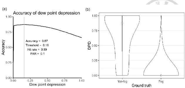
Figure 4.7 Bar plot at the best threshold of DPD (0.16).. ... 30

Figure 4.8 The fog probability in each 0.1°C interval of normalized DPD ... 32

Figure 4.9 The distribution of normalized DPD at each season. ... 32

Figure 4.10 G-mean accuracy of each threshold among seasons.. ... 34

Figure 4.11 The FEI validated by binary ground truth data, and its violin plot ... 35

Figure 4.12 (a) Bar plot at the best threshold of the FEI (2.09).. ... 35

(10)

Figure 4.15 Detail accuracy of the FEI at 2.09 threshold at MC. ... 38 Figure 4.16 Average daily number of fog event, daily fog hour, and its variance from 2018 to 2019 ... 40 Figure 4.17 Statistics of fog occurrence at each time (10 min frequency) of two year.. 41 Figure 4.18 Statistics of events by its duration for each station.. ... 43 Figure 4.19 Monthly fog probability along time showed by stations. ... 44 Figure 4.20 Comparing fog probability of four stations by season.. ... 45

(11)

List of Tables

Table 3.1 Geographical information of four meteorological stations. ... 11

Table 3.2 The accuracy matrix and definition. ... 21

Table 4.1 Spearman correlation  of four seasonal trends in Figure 4.8. ... 33

Table 4.2 DPD performance as a fog event criterion in four seasons. ... 33

(12)

1. Introduction

Forests immersed in high frequency of fog are commonly known as cloud forest. The presence of fog in cloud forests not only affects the water cycle, but heavily impacts forest structure. Cloud forests serve as vital habitats for many endemic species, including epiphytes, orchids, birds, and mammals. The high biodiversity characteristic of cloud forest makes it become the unique and important ecosystem (Aldrich et al. 1997;

Bruijnzeel et al. 2011). For example, the richness of endemic species in cloud forests was four times more than non-cloud forests of similar geographic and topographic settings (Bruijnzeel et al. 2010). Besides, fog intercepted by trunks and foliar surfaces provide not only the ecosystem additional water resources apart from rainfall but bring essential fertilizing ions to the plants rooting in the canopy and on the ground (Foster 2001;

Gottlieb et al. 2019). In the cloud forest of high altitudes, the fog water intercepted by plants may also play a pivotal role in supplying water of downstream regions (Stadtmüller 1987). Recent reports depicted that montane cloud forests were threatened due to the prevailing trend of elevated temperatures (Helmer et al. 2019). Evidences suggested that the rising of sea surface temperature is associated with fog belt shifting upward, which not only declines montane cloud forest areas but risks survival of endemic species (Ponce- Reyes et al. 2012; Pounds et al. 1999; Still et al. 1999). In addition, the general circulation models, which is popular with projecting future climatic parameters trend, suggested the scenario of warming climate in the coming decades in tropical mountains (Oliveira et al.

2014). In fact, temperature changes may cause stress on cloud forests such as shifting cloud base, altering evapotranspiration rate, impacting on hydrological cycle, and changing dominant species. In sum, cloud forests, especially tropical montane cloud

(13)

forest, which include invaluable ecological resources, are highly vulnerable to climate change (Ponce-Reyes et al. 2012).

Fog is officially defined as the visibility less than one kilometer when cloud touch the surface (NOAA 2005). In practice, the definition of fog vary from case to case (Izett et al.

2018). Its various definitions partly result from its hard-to-quantify characteristic; the first global cloud forest map was published by Bubb et al. (2004) using satellite remote sensing.

In the first cloud forest map, Asia (Insular Asia-Pacific, India, Sri Lanka, and Australia) takes the highest area proportion (nearly 60%) comparing to other continents. However, the hot spots of cloud forest studies regarding to hydrology and biodiversity are mainly conducted at Mesoamerican such as Monteverde, Costa Rica and Barro Colorado Island, Panama (Bruijnzeel 2001) of Central America. As the dynamics of fog largely being controlled by local environmental factors, the scenarios vary geographically. For example, a small mountain will experience steeper temperature lapse rate, lower sea surface temperature, and higher relative humidity than large mountain (Foster 2010). Thus, it is challenging to apply a single environmental condition to study the fog dynamic in one place, and it is urgent and needed to study fog dynamic especially in Asia.

So far, the worldwide cloud forest maps are restricted their estimated regions in the tropical areas (Bubb et al. 2004; Mulligan and Burke 2005; Wilson and Jetz 2016). It seems rational because tropical regions have the highest proportional cloud forest distribution comparing to higher latitudes areas. However, this restriction may also ignore places where are cloud forest ecosystems but outside tropics. Beyond that, it is common

(14)

cloud forest ecosystems. In fact, montane cloud forest in Taiwan not only occur in the tropics but be observed around the entire island with most of them outside the defined tropic (Schulz et al. 2017).

To date, montane cloud forest distribution can be mapped by conflating data from satellite, vegetation species, and meteorological stations with coarse resolution (more than one km).

These results reveal potential location of cloud forest globally, but lack the detailed spatial dynamic of fog at local scale. Thus, more fine-scale studies are needed to understand fog dynamics in heterogeneous mountainous regions. After all, comprehending fog dynamics reveals more detail about fog-forest interaction and their ecological effect (Weathers et al.

1986) than only identifying their location.

1.1. Research objectives

Chilan Mountain, which serves as a typical montane cloud forest ecosystem located in northeastern Taiwan, Pacific Asia, was selected as the study region. The orographic fog is more common in Taiwan than other fog types such as radiation fog in many other countries (Schulz et al. 2017). The diurnal cycle in our study area is that the air masses, which mostly come from the southeast direction lifted by orography in the evening, are cooled and condensed at the middle elevations (Klemm et al. 2006).

This study accesses this prevail fog formation (defined as cloud that touch the ground) to conduct fog duration research and attempts to achieve two objectives:

(1) Integrating satellite and in-situ meteorological data to develop the Fog Event Index (FEI), which have the ability to detect high spatiotemporal fog events.

(2) Investigating the spatiotemporal dynamics of fog duration in Chilan Mountain.

(15)

We designed a new approach, which by means of solar intensity difference as well as dew point depression to estimated 10 minutes resolution fog duration in a two year range across ~15.5 km wide region. We constrained our analyzed time within day time because the photosynthesis only happens during the day. The results can then reflect how fog interferes forest production potentially. To our knowledge, no any research have estimated this high spatiotemporal and long term period of fog dynamic at our sites before. Besides, our approach cannot provide the exact fog quantity but the highly temporal resolution duration. With the high temporal resolution fog duration along the altitudes, we can know how fog vary in montane areas, and provide a basic understanding of how much water and nutrients it potentially bring. Our estimated approach is purposed to reveal the mystery of fog in the montane cloud forest.

(16)

2. Literature Reviews

2.1. The roles of fog in ecosystems

Fog is a pivotal component to control limiting resources in cloud forests through hydrologic, nutrients, and energy cycles. These three aspects significantly related to forest growth.

Hydrologic cycle

Plants abilities to uptake water from the air enhance their survival during drought seasons and affect biotic interaction. Despite physically intercepting water in the atmosphere, over 85% of species can directly uptake it (Oliveira et al. 2014). Their absorbing strategy included by foliar and by bark (Mason Earles et al. 2016). Besides, the intercepted of fog play a water supplement role as it drip from the canopy into soil (Goldsmith et al. 2013) or go down to soil via stemflow (Hutley et al. 1997). The additional water supply to soil can be utilized by nearby root systems and understory plants. On the other hand, the presence of fog may decrease vapor pressure deficit (VPD), which affect evaporation and transpiration of plants (Burgess and Dawson 2004; Oliveira et al. 2014).

The nutrients cycle

The concentrations of both harmful and nutritious solutes (e.g. SO42-, NO3-, and NH4+) in fog were estimated to have larger amount comparing to that of in precipitation (Wrzesinsky and Klemm 2000), which can affect edaphic and physiological features of plants (Gottlieb et al. 2019). However, the chemical composition of fog shows patterns depending on local land use and location, and could vary largely among fog events (Wrzesinsky and Klemm 2000), which make them difficult to estimate. For example, coastal regions tend to experience Na⁺ and Cl^-, which come from ocean; urban and

(17)

industrial regions were recorded more sulfuric and nitric acids due to pollution;

agricultural and arid areas expose to NH4+, K⁺, Ca²⁺, and Mg²⁺because of biomass burning and dust (Weathers et al. 2020). In Chilan Mountain, chemical composition of fog shared the similar pattern (mostly SO42-, NO3-, and NH4+) as other areas but with much lower magnitude than them, which indicated higher quality of fog in this area (Chang et al. 2002). Apart from inorganic nutrients, microbes, such as bacteria, fungi, and viruses, were found that they can be transported through fog between terrestrial and marine ecosystems (Evans et al. 2019).

Energy cycle

As for energy cycle, fog water may obscure the solar irradiance, and affect plant growth and photosynthetic performance (Letts and Mulligan 2005) in both positive and negative way depending on cloud thickness, position, sun direction and plant species (Gu et al.

1999; Johnson and Smith 2008). In one scenario, the water vapor may obscure the direct solar radiation, but also gain much diffuse solar radiation, which in turn lead to total solar radiation increasing (Gu et al. 1999). In another scenario, there are also cases that fog have no effects on photosynthesis of fir seedlings or reduced photosynthesis of Rhododendron by 40% (Johnson and Smith 2008).

As a result, the interaction of the forest growth and fog presence is varying, and strongly controlled by local environmental factors and plant species. Thus, it is necessary to have long term and large scale fog event monitoring projects in different ecosystems to access the big picture of how fog events affect forest growth and the whole forest ecosystems.

(18)

2.2. Fog quantification approaches

The tiny droplets among fog and its inconstant characteristic at small local scale make the fog quantification processes full of challenges. It is hard to quantify by simple field instruments and so that make the heterogeneous montane areas unpredictable without dense data collection (Gu et al. 1999). Therefore, the studies of fog are limited compare to the studies of other much easier quantified environmental factors, like precipitation, temperature, wind speed, humidity etc. Instead of precisely measuring fog water quantity, measuring fog duration or fog frequency may be a better way to understand fog features.

Fog duration approach cannot estimate exact fog water input, yet usually can observe long-term and large spatial scale fog dynamics with lower cost. Here listed two examples of fog duration quantification methods, and their potential defects. Firstly, time-lapse photography, quantified fog frequency by continuously shooting environmental photos and classifying them into cloudy or foggy by means of cloud-sensitive image characteristics algorithm (Bassiouni et al. 2017). This method can obtain up to 90%

accuracy during both day and night, but its applicable was limited because of two reasons.

First, the parameters of cloud-sensitive image characteristics set in the study cannot widely apply to other sites. The classification results successfully test in the study would fail in another due to input solar intensity or machine specification difference. Second, time lapse camera was high battery-consume and usually without waterproof, which made it unstable in the high humidity field; The other method, time series satellite images combined with in-situ data, provided a global scale perspective about cloud forest distribution and fog frequency (Obregon et al. 2014; Thies et al. 2015; Wilson and Jetz 2016). Fog duration and frequency researches, which are conducted by satellite technology, commonly face unrefined spatial resolution challenges because fog displays

(19)

highly spatial heterogeneity over short distance.

The fog duration or the fog frequency provides a crucial clue for further estimating canopy level fog water deposition and the ecohydrology of cloud forest systems (Bassiouni et al. 2017). Their potential applications include improving performance of ecophysiological model prediction and niche-based modeling of species distribution, which are important under climate change (Oliveira et al. 2014).

2.3. Summary

Fog profoundly controlled both above and below ground parts of forests by means of regulating water, nutrient (both organic and inorganic way), and energy cycles. To know more about roles of fog in cloud forest, fog duration may be the one with less costly but the most detailed approach in the wake of satellite higher temporal and spatial resolution development. Owing to the advancement of remote sensing technology, we now can identify basic pattern of tropical cloud forests around the world using satellite imagery.

Yet its resolution part have a long way to improve, especially those cloud forest in isolated island and coastal regions. Besides, pantropical regions were needed to take into account in the context of climate change.

(20)

3. Materials and Methods

3.1. Study area

The experiments were conducted in a montane cloud forest in Chilan Mountain of northeast Taiwan (24°35′N, 121°25′E). The study area is about 16,775 ha, with altitude ranging from 1200 to 2000 m a.s.l, and approximately 50 km from the Pacific Ocean (Figure 3.1). The mean annual temperature is 13°C. Precipitation is highly variable in Chilan Mountain, which ranges from 2000 to over 5000 mm per year, depending on the amount of rainfall from typhoons in summer and northeast monsoon in winter (Chang et al. 2002). The mountainous and monsoonal features made Chilan Mountain a classic montane cloud forest (Schulz et al. 2017). The fog duration showed a strong seasonal variation. Average daily fog duration in summer was 4.7 hours, while the rest of time immersed in fog for about 11 hours per day (Chang et al. 2002). According to previous research, fog events could happen over 350 days in a single year (Chang et al. 2006), and they occurred mostly during southeastern wind direction, which was the direction of valley wind (Klemm et al. 2006). Overall, winter and spring are foggier than summer.

The frequent fog events made Chilan Mountain a typical cloud forest ecosystem. The forest canopy dominantly consists of Chamaecyparis obtusa var. formosana and Chamaecyparis formosensis (well known as Taiwan Cypress and Hinoki), with a few of Cryptomeria japonica and other broadleaf trees, which was the results of forestry history around this area.

(21)

Figure 3.1 Study area with elevation information and photos of four meteorological stations.

(22)

3.2. Meteorological data

3.2.1. Meteorological stations

Four meteorological stations were installed in winter 2017, which included three stations along forest road #100 in Chilan and a station located at forest road #110 in Mingchih (Figure 3.1). Three stations were mounted on the ground and the other one on the flux tower at ~3 m above ground. All stations were positioned without any canopy obstructed.

The stations were situated along an elevation gradient from 1151 to ~1810 m a.s.l.

(namely MC, 9K, 14.5K and 30K, Figure 3.1). The spatial extent of the stations was 15.5 km, and the slope aspect of them were different from each other (Table 3.1). The station sensors collected temperature (T, ºC), relative humidity (RH, %), rainfall (mm), and photosynthesis photon flux density (PPFD, but called PAR hereafter)( PAR Photon Flux Sensor Model S110, Decagon Devices, Inc, WA, USA) (μmol m^-2s^-1) with the time frequency of two minutes. PAR was commonly defined as wavelengths between 400 and 700 nm of solar radiation, where was the primary spectral regions for photosynthesis. We downloaded the data and checked instruments condition in the field once a month since November 2017, and 2+ years of data have been recorded. In this study, our analyzed datasets were time span from 2018/1/1 to 2019/12/31.

Table 3.1 Geographical information of four meteorological stations. From MC to 30K, the location shift from north east to south west and the elevation increase gradually.

Plot Elevation

(m)

Slope (degree)

Aspect (degree)

Longitude (E)

Latitude (N)

Mingchih 1151 3.59 184.77 121.475 24.650

9K 1514 2.64 68.50 121.448 24.598

14.5K 1670 21.76 50.82 121.415 24.590

30K 1810 3.86 223.45 121.400 24.528

(23)

3.2.2. Meteorological data gap filling

It was impractical to obtain continuous time-series meteorological data through a long period of time in forests. For instance, the high humidity and diurnal temperature range would challenge battery performance of data logger; the wild animals especially formosan reeve's muntjac in our research region liked to chew the sensor cables; some unknown reasons caused records cannot download. Data missing was inevitable.

We set a rule that if time period of missing data was less than 10 minutes, the gaps were directly applied linear interpolation for T, RH and PAR data. If the gaps were longer than 10 minutes, they were set as NA, and would not be analyzed.

3.3. Himawari-8 satellite data

3.3.1. Himawari-8 data download and retrieved

Himawari-8 (H-8 hereafter) is a Japanese geostationary meteorological satellite, which aboard Advanced Himawari Imagers (AHIs) instrument. The sensor can acquire 16 observation bands, including three visible, three near-infrared, and 10 shortwave infrared bands, with spatial and temporal resolutions of 0.5–2 km and 10 minutes, respectively (Bessho et al. 2016). With these fine resolution, the data can monitor the fluid atmospheric activities. In this study, we used the PAR product (details see section 3.5.1), which can freely download from the Japan Aerospace Exploration Agency (JAXA) P-Tree system (https://www.eorc.jaxa.jp/ptree/registration_top.html). The raw H-8 PAR products were

(24)

1985), Heliosat (Cano et al. 1986), random forest (Hou et al. 2020), and neural network (Takenaka et al. 2011). The PAR product provided by JAXA was based upon Frouin and Murakami (2007) and may meet our demand. We batch downloaded daily per 10 minutes data during daytime of Taiwan from the beginning of 2018 to the end of 2019. For each image, the PAR pixel values of geographically corresponding meteorological stations were retrieved with Matlab (MATLAB v. R2018b). After that, we can get two years’ time series PAR of four stations. The values at 10:40 local time everyday were continuing missing due to technical problem. The missing value sometimes also occurred randomly.

Because the missing time period was short, we applied liner interpolation to make it a completed two year PAR time series data.

3.3.2. Daytime period setup and Himawari-8 PAR performance

Only daytime period was analyzed because photosynthesis can solely occur during daytime, and fog events may disturb this forest growth cycle. In fact, daytime periods were different between each day especially the pronounced seasonal variance so it was not suitable to define a universal daytime period. For convenience's sake, a universal daytime period was selected first, and then the unique daytime of each day was defined by solar zenith angle lower than 90 degree based on the universal period. The universal period was defined by in-situ to H-8 PAR ratio lay between 0 and 1, which happened mostly during 6 a.m. to 6 p.m. Both in-situ and H-8 PAR values outside this time range tended to close to 0, and made the ratio unexplainable. After that, solar zenith angle with 10 minute frequency everyday was computed:

cos Z = sin ∅∙ sin δ+ cos ∅∙ cos δ∙ cos h ,

∅=latitude, δ=solar declination, h=solar hour angle

(3-1)

(25)

δ= sin^-1(0.39785∙ sin ((

278.97+0.9856∙DOY+

1.9165∙ sin ((356.6+0.9856∙DOY)∙ π

180)) ∙ π

180)) ∙180 π

(3-2)

h=(time-t0)∙15, time=local time (3-3)

t0=12-LC-ET, LC=longitude correction, ET=equation of time (3-4) LC=(longitude-Standard longitude)

15

(3-5)

ET=

-104.7∙sin(f)+596.2∙sin(2∙f)+4.3∙sin(3∙f)- 12.7∙sin(4∙f)-429.3∙cos(f)-2∙cos(2∙f)+19.3∙cos(3∙f)

3600

(3-6)

f=(279.575+0.9856∙DOY)∙ π

180 (Degrees) (3-7)

Solar zenith angle = cos^-1Z ∙ ^𝜋

180 (Degrees) (3-8)

In addition, the performance of Himawari-8 was checked before further analysis. In fog- free condition, Himawari-8 PAR value should be close to in-situ PAR value while in the foggy condition, two values would be distinct as a result of sunlight blocking by fog. The relationship of Himawari-8 PAR and in-situ PAR during fog-free and foggy condition were analyzed respectively. Their root mean square error (RMSE) and rRMSE were presented in results section. The RMSE and rRMSE are defined as follows:

𝑅𝑀𝑆𝐸 = √∑^𝑁_𝑖=1(𝑦_𝑖 − 𝑦̂ )_𝑖 ² 𝑁 𝑟𝑅𝑀𝑆𝐸 = 𝑅𝑀𝑆𝐸

𝑦̅_𝑖

Where 𝑦_𝑖 is the ith in-situ PAR value, 𝑦̂ is the corresponding H-8 PAR value, N is the _𝑖 total number of observation, and 𝑦̅ is the mean of in-situ PAR value. _𝑖

(26)

3.4. Validation data

There were two time lapse cameras. The first time lapse camera (Brinno TLC200 PRO) was installed at 14.5K station since 2018 for model development and validation, and the second camera (Bushnell Trophy Cam) was mounted at MC station since mid-March 2020 for additional validation. The detailed validated process would be provided in section 3.5.2. The time lapse cameras were set to collect image every 10 minutes during day time only (6 a.m. to 6 p.m.), and can be played in Brinno Video Player software with timestamp at each image bottom. We repeatedly changed SD card and batteries of the camera, and checked the machine condition monthly. To decide if fog occur or not, we visually classified each image into two categories, which was true for fog occur and false for the fog-free condition (Figure 3.2). The standard was that if cloud bottom touch the mountain top of the images, then set as fog event. With this approach, we can get a binary ground truth time series data about fog events for 14.5K and MC stations respectively.

Figure 3.2 Examples of (a) fog-free situation and (b) foggy moment. Following our classified standard (a) would be set to false while (b) would be true.

3.5. The FEI development

Before further analyzing, it was necessary to integrate different time series data into the

(27)

same temporal resolution. Thus, the coarsest resolution among all dataset, 10 minutes, was chosen. All meteorological variables, T, RH, and PAR were aggregated to 10 minutes resolution.

In order to obtain daily fog duration, we firstly built a fog event index model by H-8 PAR product, and in-situ meteorological data (T, RH, and PAR) in the 14.5K station, and validated the model by time lapse video binary time series data (binary ground truth hereafter). With the binary ground truth data, we can find a threshold that resulted in the highest accuracy. The models were then developed and threshold was applied to other meteorological stations (MC, 9K, and 30K). The MC station was validated again at this step to check the model performance (Note that we used 2020/3/17 to 4/12 binary ground truth as validation data). Finally, we would generate daily fog duration time series data for four stations, and discuss how the environmental factors, such as altitudes and aspect, influence fog pattern, and analyze the fog seasonal patterns within each station.

3.5.1. The FEI model

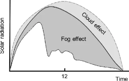
When fog occurred, there were two significant environmental changes: solar intensity and humidity. As for solar intensity attenuation caused by fog events, our computed approach was illustrated in Figure 3.3. In fog-free condition, the PAR value in the sky should be close to that of on the ground. In contrast, in a foggy condition, water vapor will block out most of sunlight. Thus, the PAR at canopy level should be much lower than that of in the sky. Hence, we can trace when the fog onset does by computing the difference of PAR in the sky and on the ground. However, the PAR value in the sky was heavily affected by

(28)

then compare H-8 PAR to in-situ PAR to trace the exact fog onset moments. The advantage of tracing PAR rather than shortwave radiation was that PAR directly reflected source of energy for photosynthesis.

Figure 3.3 The black dash line indicated in-situ PAR value, and the black solid line represented PAR value under cloud, which was obtained by H-8 PAR product. The grey dash line in the background showed model estimated value without considering cloud appearance.

The major concept of our model was to capture solar intensity and humidity changes while fog occurred. Thus, two criteria were set:

(1) The ratio of in-situ PAR to H-8 PAR. (PAR ratio)

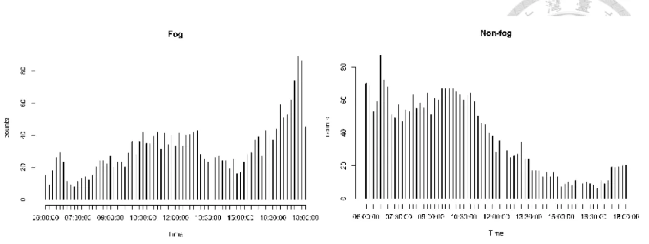
The results should lie in range 0 to 1, but value larger than 1 could happen sometimes.

The empirical data showed that when value larger than 1 occurred, it would be higher probability it was fogless situation before 12 p.m., but in foggy situation after 12 p.m.

(Figure 3.4). Thus, if the ratio was larger than 1, then set to 1 when it happened before 12 o’clock, and set to 0 when in the afternoon. The value should be closer to 1 in fog- free condition and down to 0 in fog event.

(29)

Figure 3.4 The ratio of H-8 to in-situ PAR, which larger than one, were divided into two groups by binary ground truth data.

(2) Dew-point depression (DPD).

Dew point temperature (Td hereafter) is a threshold where water vapor will condense into liquid water. The equation of dew point temperature is:

𝑇𝑑 = 𝑏 [ ln 𝑅𝐻 100 +

𝑎 𝑇 𝑏 + 𝑇 ] 𝑎 − ln𝑅𝐻

100 − 𝑎 𝑇 𝑏 + 𝑇

where a is 17.27 and b is 237.7 (Barenbrug 1965). The unit of RH is percentage and T is °C respectively. After computing the Td time series by T and RH data, we created a dew-point depression index (DPD hereafter) calculated by T minus Td. For some outlier less than 0, we set them to 0 manually. Thus, the larger the DPD, the more confident that it is fogless. The threshold where fog onset depends on local weather condition. Generally it was set to lower than 0.5–2.5 °C (Hiatt et al. 2012; Veljović et al. 2015). The reasons why DPD was used as an indicator instead of RH were that firstly over three quarters of our RH values were larger than 90%. The non-uniform

(30)

moisture. Since DPD can range from 0 to a large number (e.g. ~30°C in our empirical data), the normalize process was necessary. In order to diminish outlier effect, the maximum value to normalize was set as 2.5°C rather than empirical maximum value.

The normalize formula is:

DPDnormalize = 𝐷𝑃𝐷 − min (𝐷𝑃𝐷) 2.5 − min (𝐷𝑃𝐷)

To those value larger than 1 after normalization, we set them to 1 uniformly. Thus the range of DPD normalization would between 0 and 1.

After calculating these two indicators for the 14.5K station, we got two time series data following identical rule that the larger their value, the more confident fogless condition at that moment. Therefore, a new indicator was created by add up the fraction of these two time series data minute by minute. The coefficient a and b represent the best thresholds of two indicators, which would be determined by binary ground truth data in the next subsection:

Fog Event Index (FEI) = 1

𝑎∙ 𝑃𝐴𝑅 𝑟𝑎𝑡𝑖𝑜 +1

𝑏∙ 𝐷𝑃𝐷𝑛𝑜𝑟𝑚𝑎𝑙𝑖𝑧𝑒𝑑

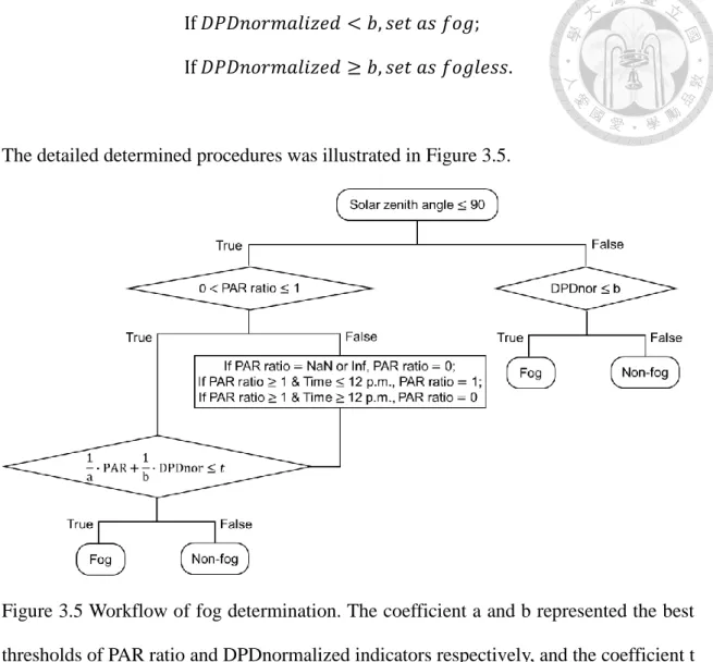
We can get a new time series called fog event index, and again, the larger the FEI, the more likely they are fogless condition. The concept that each indicator firstly compared to their best threshold, and sum, can ensure the FEI would not be dominated by any particular indicator. Besides, the thresholds, which were determined by the physical characteristics of solar radiation and dew point depression, would not vary during climate change scenario. In theory, as long as the FEI is larger than 2, it can be viewed as fog occur. For those moments that lay in 6 a.m. to 6 p.m. but their solar zenith angles were larger than 90 degree, their fog condition would be decided by the DPDnormaized indicator only. Their decision process can be described as:

(31)

If 𝐷𝑃𝐷𝑛𝑜𝑟𝑚𝑎𝑙𝑖𝑧𝑒𝑑 < 𝑏, 𝑠𝑒𝑡 𝑎𝑠 𝑓𝑜𝑔;

If 𝐷𝑃𝐷𝑛𝑜𝑟𝑚𝑎𝑙𝑖𝑧𝑒𝑑 ≥ 𝑏, 𝑠𝑒𝑡 𝑎𝑠 𝑓𝑜𝑔𝑙𝑒𝑠𝑠.

The detailed determined procedures was illustrated in Figure 3.5.

Figure 3.5 Workflow of fog determination. The coefficient a and b represented the best thresholds of PAR ratio and DPDnormalized indicators respectively, and the coefficient t was the best threshold of the FEI model.

3.5.2. Two indicators validation and assessment of the FEI performance

Before running our model, PAR ratio and the DPD time series data were individually validated by binary ground truth data to check how much they potentially contributed to the model, and get their best thresholds for the FEI usage. In addition, the DPD was further test for their seasonality.

(32)

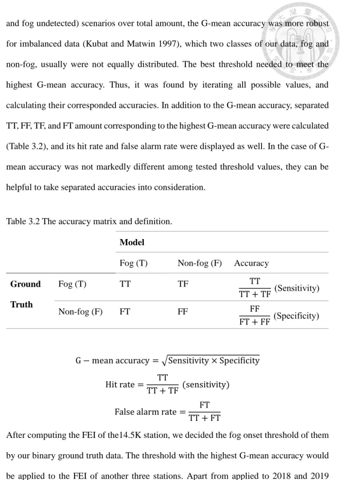
and fog undetected) scenarios over total amount, the G-mean accuracy was more robust for imbalanced data (Kubat and Matwin 1997), which two classes of our data, fog and non-fog, usually were not equally distributed. The best threshold needed to meet the highest G-mean accuracy. Thus, it was found by iterating all possible values, and calculating their corresponded accuracies. In addition to the G-mean accuracy, separated TT, FF, TF, and FT amount corresponding to the highest G-mean accuracy were calculated (Table 3.2), and its hit rate and false alarm rate were displayed as well. In the case of G- mean accuracy was not markedly different among tested threshold values, they can be helpful to take separated accuracies into consideration.

Table 3.2 The accuracy matrix and definition.

Model

Fog (T) Non-fog (F) Accuracy Ground

Truth

Fog (T) TT TF TT

TT + TF (Sensitivity)

Non-fog (F) FT FF FF

FT + FF (Specificity)

G − mean accuracy = √Sensitivity × Specificity Hit rate = TT

TT + TF (sensitivity) False alarm rate = FT

TT + FT

After computing the FEI of the14.5K station, we decided the fog onset threshold of them by our binary ground truth data. The threshold with the highest G-mean accuracy would be applied to the FEI of another three stations. Apart from applied to 2018 and 2019 dataset of the other three stations, the model at the MC station from 2020/3/17 to 4/12 was also applied with the same threshold to confirm the model performance in elsewhere.

(33)

Due to experimental design, the validated data was limited in spring at MC so far.

3.6. Application of the FEI

After thresholds of the FEI were set, the FEI of all stations were computed and allowed to further analyze their environmental factors and seasonality. Average daily fog event and average daily fog hours of each month were presented. The fog duration frequency and fog seasonality of each site were showed as well.

(34)

4. Results

4.1. Meteorological data

The missing records of two minutes frequency raw data were 5%, 7%, 8%, and 10% at MC, 9K, 14.5K, and 30K respectively. We have totally 53,290 records with two year 10 minutes frequency dataset for each meteorological station counting during 6 a.m. to 6 p.m.

Besides, there are 2,209 records with the 10 minute frequency dataset at the MC station during daily 6 a.m. to 6 p.m. in 2020 as well.

4.2. Himawari-8 satellite data

4.2.1. Daytime period setup and Himawari-8 PAR performance

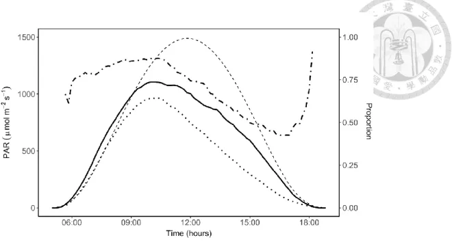
The definition of daytime range came from the result of Figure 4.1. In dot-dash line of Figure 4.1, the proportion kept stable before 10:30 a.m. After that, it started to decline and reached its minimum at about 4:30 p.m. Finally, a sharp increase climbed back to morning level. These dynamic indicated the time between10:30 and 16:30 was favored by fog events. The lower proportion may imply more frequent fog events at that time.

Since the average proportion of PAR ratio during the time span of 6 a.m. to 6 p.m. lay between 0 and 1 (Figure 4.1), it was reasonable to set this time span as our universal daytime. Besides, solar zenith angle, which lower than 90 degree, played the second threshold as daytime determination. For example, the daytime was from 6 a.m. to 6 p.m.

in summer solstice of 2018 (6/21) while it was from 6:40 a.m. to 5 p.m. in winter solstice of 2018 (12/22).

(35)

Figure 4.1 Two-years average PAR with 10 min frequency at 14.5K. The symmetry curve at the background indicated ideal situation when it was clear sky, and reached the highest PAR at noon. The solid line indicated H-8 PAR, which represented the value under cloud effect. Values were observed slightly higher than ideal situation before 9 a.m., which may cause by topography effect or terrain heterogeneity. The dotted line indicated in-situ PAR.

Both H-8 and in-situ PAR showed asymmetry curve. The dot-dash line represented in- situ to H-8 PAR ratio, and corresponded to the right Y- axis.

(36)

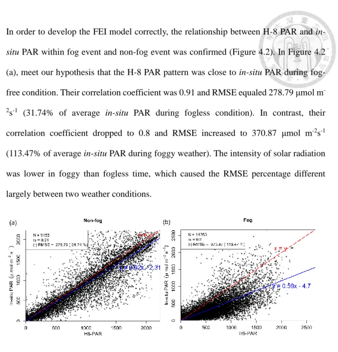
In order to develop the FEI model correctly, the relationship between H-8 PAR and in- situ PAR within fog event and non-fog event was confirmed (Figure 4.2). In Figure 4.2 (a), meet our hypothesis that the H-8 PAR pattern was close to in-situ PAR during fog- free condition. Their correlation coefficient was 0.91 and RMSE equaled 278.79 μmol m^-

2s^-1 (31.74% of average in-situ PAR during fogless condition). In contrast, their correlation coefficient dropped to 0.8 and RMSE increased to 370.87 μmol m^-2s^-1 (113.47% of average in-situ PAR during foggy weather). The intensity of solar radiation was lower in foggy than fogless time, which caused the RMSE percentage different largely between two weather conditions.

Figure 4.2 Classifying ground truth time series into fog and non-fog events according to binary ground truth data, the relationship between H-8 PAR and in-situ PAR when fog- free condition are showed in (a), while that of when fog events are showed in (b). N means record numbers, rs indicates the spearman’s rank correlation, and RMSE represents root mean square error. Data followed the red dash line (1:1) closer during non-fog events, which guaranteed accuracy of H-8 PAR.

(37)

4.3. Validation data

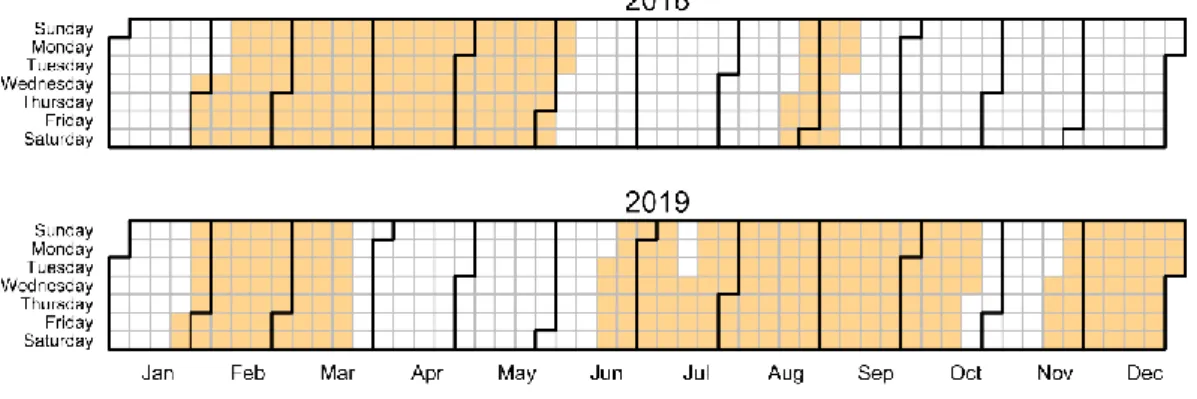
Due to some inevitable camera malfunction, the total length of available binary ground truth data was about one year. Fortunately, the available time-series data covered different seasons, which would lower the bias to the situation which only have available data cluster in certain seasons (Figure 4.3). The total binary ground truth data have 26,425 records with 10 minutes frequency, which included 16,302 fog event records (~62%) and 10,123 non-fog records (~38%).

Figure 4.3 The orange color blocks in the calendar indicated the time lapse camera successfully recorded date in 2018 and 2019. The total recorded date number were 367 days, which was about half of 14.5K dataset.

As for the MC station, there were totally 2,209 records, which included 1,084 fog event records (~49%) and 1,125 non-fog records (~51%). Due to our limitation of data collected design, the validation data at MC station mainly occurred in spring.

(38)

4.4. The FEI development

4.4.1. Two indicators validation and assessment of the FEI performance Two indicators validation

Before developing the FEI model, we also individually validated two criteria by binary ground truth data in advance to know each of their potential contribution to the model.

The same process was repeatedly applied, and showed in the lists below. Firstly, we divided the criteria time series data into fog and non-fog groups by binary ground truth data, and draw the violin plot. If the criterion was a good estimator, the distribution position should distinct. Secondly, we iterated all possible thresholds, and calculated the G-mean accuracy in each iteration. In this stage, the best thresholds, the G-mean accuracies, hit rate, and false alarm rate will be presented. The bar plots were illustrated to demonstrate detailed accuracy at the best threshold.

(1) The ratio of in-situ PAR to the H-8 PAR (PAR ratio)

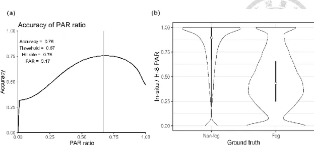
The distinct position of each group (Figure 4.4 (b)) indicated the potential well perform of this criterion. In Figure 4.4 (a), we knew that the highest G-mean accuracy (~76%) occurred at 0.67 threshold. This 0.67 would become the value of coefficient

“a” in the FEI model. Its detailed performance at 0.67 threshold showed in Figure 4.5.

The percentage of true positive and true negative both were more than 75 %. In addition, there were 83% accuracy in the fog detected scenario, but the accuracy declined to 67% in the fog undetected scenario, which namely there was 34% non- fog detected data (PAR ratio larger than 0.67) actually was immersed in fog.

(39)

Figure 4.4 The ratio of in-situ PAR to H-8 PAR validated by binary ground truth data. (a) Iterating all possible thresholds and marking the highest G-mean accuracy, at threshold 0.67 showed ~76% accuracy. (b) Divided the ratio data into fog and non-fog by binary ground truth data. The non-fog group was distributed higher than the fog one, but two groups were not totally separate distribution.

Figure 4.5 (a) Bar plot at the best threshold (0.67). Larger than the threshold means estimated non-fog condition while lower indicated estimated foggy events. X-axis was binary ground truth data, and y-axis was probability. (b) Detailed bar plot at the best

(40)

(2) The dew point depression (DPD)

The second criterion was a direct and traditional approach to detect humidity. In Figure 4.6 (b), Distribution of normalized DPD value separated clearly in foggy and fog-free condition. Despite some outliers in the fog event group, their mean was largely different, and the lower quartile of non-fog was far larger than the third quartile of fog event. In Figure 4.6 (a) the highest total accuracy (87%) occurred at 0.16. This value became the coefficient “b” in the FEI model. In Figure 4.7, the detail accuracy improved compared to the accuracy of PAR ratio. For example, the percentage of true positive and true negative both were more than 85 %, and both hit rate (89%) and false alarm rate (10%) indicated normalized DPD could be a reliable indicator for detecting fog event.

(41)

Figure 4.6 DPD validated by binary ground truth data. (a) Iterating thresholds and marking the highest G-mean accuracy, at threshold 0.16 showed 87% accuracy. (b) Divided DPD into fog and non-fog by binary ground truth data.

Figure 4.7 (a) Bar plot at the best threshold (0.16). Larger than the threshold means estimated fog-free condition while lower indicated estimated foggy. The x-axis was binary ground truth data, and y-axis was probability. (b) Detailed bar plot at the best threshold too, and x-axis was separated by model value.

(42)

Seasonality of DPD

It was worth to mention that the seasonality of normalized DPD was not significant enough to affect our result when a single threshold was applied to whole year. In Figure 4.8, fog probability, which was validated by binary ground truth data, decreased linearly from zero to one interval. Fog probability was the total fog event records divided by total events within a DPD bin. The decreasing speed of four seasons from slow to fast order by spring, summer, fall, and winter. Trends of four seasons were strongly correlated statistically (spearman  >= 0.99, p value < 0.001) (Table 4.1), which indicated seasonality may be negligible. There detailed comparison showed in Table 4.2. The best threshold was close to the whole dataset value (0.16) only in summer (0.15) while the best thresholds in spring (0.34), fall (0.04), and winter (0.02) were different from the whole dataset value. The difference of spring, fall, and winter threshold may result from two reasons. Firstly, the fog event frequency was different among seasons in reality. In our case, the best threshold in spring (0.34) was more than two times higher than the universal threshold (0.16), and it decreased progressively until winter. This may indicate winter was much more prevalent to fog event. The second reason may be the validation dataset biased (Figure 4.9). The proportion of fog events in whole data among each season were demonstrated in Table 4.2 (the N of fog row). The proportion of fog events toke more than 60% in summer to winter and whole dataset except spring (54%). This fact could simultaneously bias the best threshold training, and be the proof of less fog event in spring.

Despite this, we applied the universal threshold (0.16) directly to each season and got their G-mean accuracies all larger than 86% Table 4.2 (the accuracy at 0.16 row), which was not their best performance, but was still acceptable. The results of G-mean

(43)

accuracy among seasons iterated from zero to one showed in Figure 4.10. With this evidences, applying a universal threshold to different seasons should be legitimate.

Figure 4.8 The fog probability in each 0.1°C interval of normalized DPD, which was validated by binary ground truth data at 14.5K station. Seasonality was not significant among four seasons.

Figure 4.9 The distribution of normalized DPD at each season. The circle was mean, and the triangle was median. The median was zero in all seasons except spring.

(44)

Table 4.1 Spearman correlation  of four seasonal trends in Figure 4.8.

Spring (3,4,5)

Summer (6,7,8)

Fall (9,10,11)

Winter (12,1,2)

Spring 1 1 0.99 0.99

Summer - 1 0.99 0.99

Fall - - 1 0.96

Winter - - - 1

Note: p value all < 0.001.

Table 4.2 DPD performance as a fog event criterion in four seasons.

Spring Summer Fall Winter Whole N

(without gap data)

6552 6128 5387 6393 24460

N of fog (prop. of N)

3559 (0.54)

3840 (0.63)

3584 (0.67)

3912 (0.61)

14895 (0.61) Threshold/Optim G-

mean Accuracy

0.34/0.88 0.15/0.86 0.04/0.88 0.02/0.88 0.16/0.87

Accuracy at 0.16 0.87 0.86 0.87 0.87 0.87

(45)

Figure 4.10 G-mean accuracy of each threshold among seasons. The grey vertical line indicated the universal threshold (0.16).

To sum up, between these two criteria, the normalized DPD demonstrated better estimation with ~87% total accuracy, while the ratio of in-situ to H-8 PAR with ~76%

accuracy.

Assessment of the FEI performance

After PAR ratio and normalized DPD were individually validated, they were separately multiplied by their reciprocal of best threshold, and added up to form the FEI. The assessment process was similar to individual criterion validation, which iterated possible values and found the best threshold corresponding to the highest G-mean accuracy. In Figure 4.11 (a), the optimal threshold lay in 2.09 with ~87% accuracy, and the FEI distribution by groups illustrated in Figure 4.11 (b). The accuracy did improve from

(46)

true positive, which rose from 0.89 of DPD criterion to 0.9 of the FEI. The hit rate of the FEI (0.9) improved compared to individual PAR ratio (0.76) or normalized DPD (0.89) indicator.

Figure 4.11 The FEI validated by binary ground truth data. (a) Iterating thresholds under 7.5 unit and marking the highest G-mean accuracy, at threshold 2.09 showed ~87%

accuracy. (b) Divided the FEI into fog and non-fog by binary ground truth data.

Figure 4.12 (a) Bar plot at the best threshold (2.09). Larger than the threshold means estimated fog-free while lower indicated estimated foggy. X-axis was binary ground truth data, and y-axis was probability. (b) Detailed bar plot at the best threshold too, and x-axis was separated by model value.

(47)

Results of error distribution at each time with 10 minutes frequency showed in Figure 4.13. An ideal model should be evenly distributed error through time. In Figure 4.13 (a), an obvious decreasing pattern showed before 9:00 a.m., and a rising pattern after 5 p.m.

was observed. The dynamics may be caused by droplets of dew stick to sensor surface at dawn or dusk and distorted the value. In Figure 4.13 (b), regardless the PAR ratio or normalized DPD, both of them showed the bell curve with reaching the highest error count around noon. This evidence may indicate that fog events around noon were thin, and their signals were too weak to detect. Thus, if we sum false positive and false negative together, early morning, late evening and noon demonstrated slightly higher error pattern.

This model showed another important phenomenon that error of the FEI followed strongly on the normalized DPD criterion. This indicated that normalized DPD was much more dominant than PAR ratio did in this model

Figure 4.13 The proportion of error at each moment. (a) Displayed false positive situation that binary ground truth found fogless but model detected fog. FEI: the fog event index;

Ratio: in-situ to H-8 PAR ratio. (b) False negative situation. (c) Sum of (a) and (b). Note that because solar zenith angle varied among seasons, the total records at each time would

(48)

Validation at MingChih

The best threshold of PAR ratio and the normalized DPD at MC were 0.39 and 0.21 respectively, but the coefficient a (0.67) and b (0.16) were applied at 14.5K replaced the best threshold of MC here. In Figure 4.14 (a), the highest G-mean accuracy was 85%

occurred at 1.78 threshold, which was slightly lower than expected value (2) and 14.5K empirical threshold (2.09). The accuracy was declined to ~82% at 2.09, but still acceptable. Therefore, this step displayed the fog detected capability of the FEI with universal threshold not only limited at its built station, 14.5K, but also can extend to other regions.

(49)

Figure 4.14 Applying coefficient a and b from 14.5K empirical threshold to compute the FEI. (a) Iterating all possible thresholds of the FEI and marked the corresponding G-mean accuracy at threshold 1.78. (b) Divided the FEI into fog and non-fog by binary ground truth data.

Figure 4.15 Detail accuracy of the FEI at 2.09 threshold.

(50)

4.5. Application of the FEI

Fog duration at each station

At the monthly time scale, event variation between months were high at MC and 30K while they were low at 9K and 14.5K (Figure 4.16 (a)). In Figure 4.16 (b), the error bars, which indicated standard deviation of each fog duration monthly, revealed the characteristic of fog event length. Fog duration tent to have higher variation in winter than summer. Besides, the average daily fog duration between months roughly showed pattern of winter lasting longer than summer at all stations. For summer of the MC station, the estimated results were nearly fogless. In Figure 4.16, the average daily fog events were high in winter of MC and 30K, but the average daily fog hour were relative low in winter of both comparing to 9K and 14.5K. This pattern indicated that fog formation condition stuck in a cycle of being satisfied and unsatisfied at that time.

In addition, two visually groups formed, 9K and 14.5K at more fog group while MC and 30K at less fog group. The groups may result from elevation difference. The more fog group situated at middle elevations (~1514~1670 m a.s.l.), which was favored to fog formation. The largest value of average daily fog hour was 10.5 hours, which happened at 9K in January. This results were similar with previous research near our study area, which suggested that average daily fog duration of non-summer month was 11 hours (Chang et al. 2002). In fact, the value can reach over 12 hours at least for four months in previous results nearly 20 year ago while only one site and a month of our result was over 10 hours. Also needed to note that the previous research took 24 hours in account, but our results only considered half of day. The total duration hours of two year time span were 1510, 5625, 5257, and 1446 hours at MC, 9K , 14.5K, and 30K respectively. But note that the proportion of gap data were 5%, 7%, 8%, and 10% at four stations respectively. The

(51)

total duration hours of maximum station (9K) was ~3.9 times of that of minimum one (MC).

Figure 4.16 Average daily number of fog event from 2018 to 2019 showed in (a). (b) Average daily fog hour. The error bars indicated the variation of fog duration

Scanning through fog event by moment of each day, the pattern was clear and identical among four stations (Figure 4.17). Moments closed to sunrise and sunset tent to have higher opportunity to occur fog while moments before noon were not favored by fog. The visually groups here were more obvious. In regards to the special pattern of 14.5K before noon, it may stem from station position. The 14.5K station was the only station that mounted its sensors on top of a tower whereas other stations were installed on the ground.

Higher sensors position may lead to delay of DPD decreasing because water vapor was assumed to evaporate form ground or canopy to higher air. After around 10 a.m., this delayed phenomenon vanished. The probability of fog at 14.5K increased and even exceeded MC as the highest place lasting until the end of a day.

(52)

Figure 4.17 Statistics of fog occurrence at each time (10 min frequency) of two year. X- axis was counts and y-axis was converted into fog occur probability. The error interval of 14.5K was showed in the grey area (under interval: proportion of false positive; upper interval: proportion of false negative).

(53)

All of stations share comparable decreasing pattern that most of the fog events lasted less than an hour, and the longer the fog event the fewer time it happen. Since we only counted time between 6 a.m. and 6 p.m., the value at bin larger than 12 hours represented days that experienced fog with the whole moments. The fog situation in Chilan Mountain tent to be either short-time fog or lasting for whole day long. There were few cases that fog lasted for more than eight hours or more, and mixed with fogless situation in a single day.

The spike at bin larger than 12 hours occurred at whole year of all stations (Figure 4.18(b)), and only occurred at the four seasons of more fog group (Figure 4.18(a)). Average rainfall of each station with whole day fog (>12hrs), and with whole condition were 8.3/10.3, 5.7/11.5, 6.6/9.3, 5.6/9.5 respectively. Thus, the cause of the spike was not by rainfall.

(54)

Figure 4.18 Statistics of events by its duration. These were two year results at four stations respectively. Y-axis was power to base 10. (a) Four seasons event frequency at each station. (b) Whole year event frequency at each station.

(55)

Seasonality of fog

The fog probability at each month along each station showed in Figure 4.19. Almost all stations displayed phenomenon that winter with higher fog occurrence while summer with the lowest fog occurrence. The afternoon of 14.5K showed the lack of seasonality.

If we switched our perspective from station base to seasonal base, in season difference among four stations were compared in Figure 4.20. The visually more fog and less fog groups observed form previous section can still be found in each season.

Figure 4.19 Monthly fog probability along time showed by stations. X-axis indicated month, y-axis represented time summarized by two year data, and z-axis was probability.

Figure order: (top left: MC, top right: 9K, bottom left: 14.5K, bottom right: 30K)

(56)

Figure 4.20 Comparing fog probability of four stations by season. X-axis indicated 10 minutes frequency of time, and y-axis represented fog probability summarized by two year data.

(57)

5. Discussion

We developed a new model, the FEI, to detect daytime fog event in high spatiotemporal resolution, which revealed fog duration dynamics of montane cloud forest of Taiwan for the first time. This section will discuss the uncertainties of our model, its potential application, fog characteristic in Chilan Mountain, and our limitation.

5.1. The FEI performance and its application

5.1.1. The causes of uncertainties

The FEI is composed of PAR ratio and normalized DPD to identify fog event. The uncertainty of PAR ratio may be caused by the different capability of fog density to obscure the solar irradiance, and the 5 km resolution of H-8 PAR compared to single point in-situ PAR data. There are 9% uncertainty between H-8 PAR and in-situ PAR during fogless condition Figure 4.2 (a), and 70% of H-8 PAR overestimate in-situ value, which could be the reason accuracy of non-fog condition is worse than foggy condition. On the other hand, except for detecting fog water, DPD may be influence by rain. Thus, considering both criteria at the same time can cover up each disadvantage. As for the times when solar zenith angle is larger than 90 degrees, normalized DPD becomes the only criterion. They may be affected by rainfall.

The uncertainties of the FEI varying along time, which the false positive signals tend to occur at dawn and dusk, and the false negative signals tend to occur at noon (Figure 4.13 a & b), are unavoidable. The false positive situation may be caused by residual water

(58)

5.1.2. Contribution of two indicators

Although the normalized DPD outperformed PAR ratio more than 10%, it cannot be directly linked to the result that normalized DPD was more sensitive to fog events than solar intensity did. It was important to keep in mind that the relationship between H-8 PAR and fog-free in-situ PAR was 0.91 Figure 4.2 (a). If the resolution of satellite data improved, the ability of PAR ratio indicator may expectedly perform well like the normalized DPD did. So far, the outperforming normalized DPD may lead to subtle fog- detected difference between normalized DPD and the FEI. Yet the PAR ratio currently got 76% of accuracy, which also can be viewed as strong estimators. With the more precise under-cloud PAR data in the future, the contribution of PAR ratio indicator is looking forward to increasing.

5.1.3. Applicability of the FEI

Cloud is the most challenge factor that affect fog detection research. Previous fog detection using only remote sensing data can obtain a large scale fog dynamics but faced challenges such as cannot distinguish fog and low stratus cloud (Egli et al. 2018) and spectrum interfere by cloud(Andrews and Bright 2018). However, the PAR ratio indicator can theoretically avoid cloud effect to detect fog event. With our hybrid ground and satellite data method, the hit rate of fog event largely increases (87%) comparing to that applying bispectral image processing method (69%) (Andrews and Bright 2018). Yet the accuracy improves by hybrid method, the density of in-situ data will determine the spatial resolution of fog dynamic. Thus, there is a trade-off between accuracy and spatial resolution. The FEI only needs to set an open-sky metrological station with common meteorological sensors to detect fog, which will be far more convenient than maintaining

(59)

a visibility sensor on a flux tower.

5.2. Fog characteristic in Chilan Mountain

5.2.1. Aspects and altitudes

Aspect and elevation are two important factors that strongly control fog duration. Based on existing analysis, fog duration of ocean-faced sides are much longer than the opposite sides. However, it need further confirmation with the wind speed dataset because the overall aspect is hard to define in a heterogeneous mountain terrain.

Fog generally form at between 1500 and 2500 m.a.s.l. in Taiwan, but vary because of aspect or mountain size difference (Schulz et al. 2017). Our experimental design considering practice limitation set the altitudes ranging from 1151 to 1810 m a.s.l. (~660 m), which already lies in the general altitude range. According to our results, the fog duration can vary a lot inside fog occurrence zone. The more fog group lay in northeast side of ~1514 and ~1670 m.a.s.l., which water vapor may come with see breeze, and format fog at the middle elevations. If the exact boundary of fog belt zone is wanted, more windward sensors need to be added in the future, which one locate at lower than 1515 m a.s.l. while another one locate at higher than 1670 m a.s.l.

5.2.2. Fog duration pattern

All of our stations showed short period fog event, which less than an hour long, was more frequent, and the event frequency decreased gradually while duration get longer. However, event with whole day immersed in fog (>12 hrs) rose (Figure 4.18), which especially