利用單眼視覺之增強性方向梯度直方圖於多人偵測

(1)

國立臺灣大學電機資訊學院資訊工程學研究所碩士論文

Department of Computer Science and Information Engineering College of Electrical Engineering ＆ Computer Science

National Taiwan University Master Thesis

利用單眼視覺之增強性方向梯度直方圖於多人偵測

Monocular Multi-Human Detection Using Augmented Histograms of Oriented Gradients

莊振勛

Cheng-Hsiung Chuang

指導教授：傅立成博士 Advisor: Li-Chen Fu, Ph.D.

中華民國 97 年 6 月

June, 2008

(2)

誌謝

充實的碩士班生涯即將結束，馬上就要走入人生另一個旅程，回顧碩士班的兩年生涯，大大小小的事都足以令我回憶一生。不論是和大家一起熬夜寫作業趕計畫，一起在球場上揮灑汗水，或是失落時互相鼓勵的場景，都是我人生中的珍貴回憶。

碩士班生涯中，最感謝的人莫過於指導教授傅立成老師。他秉持嚴格的研究訓練及強調團隊合作與時間分配的態度養成，令我受益良多，並且在我遭遇挫折時，不斷給予我指導及鼓勵，使我能繼續堅持下去。同時感謝學長黃世勳教授在我剛進入碩士班時的細心指導，讓我很快地熟悉實驗室的大小事，以及帶領我進入研究的殿堂，除此之外，亦感謝洪一平教授、蕭培墉教授及陳祝嵩教授審閱全文，並給予許多寶貴的意見與指正，使得本論文能更加完善。

求學路途走來跌跌撞撞，感謝父母不斷的給予我安慰及支持，在我茫然不知所措時，能很快找到自己的方向。感謝兩位姐姐給我的支持與鼓勵，有家人的支持我才能無後顧之憂的完成碩士班的學業。感謝女友心懿在我最辛苦的關頭，一直陪在我身邊，照顧我、包容我。

感謝機器人實驗室的影像組成員：益銘學長、一航、忞蔚、思穎。能與各位互相討論研究，一起完成一項工作的過程，讓我學到一個人如何與團隊間其他人相處。育誠、禹安、佳委、嘉鳴，有你們的存在，讓我在最後奮戰的路途上有相互扶持的夥伴。同時亦感謝實驗室的其他成員：開哥、兆麟、恩暐、小陸、峻鋒、

士桓、阿擂、馬卡卡、意函、學謙、亞文，不僅在學業上的相互砥礪，同時增加了我許多的生活樂趣，最後感謝助理們：小寧，郁璇、懿萱、立婷協助我處理實驗室的大小事，讓我能更專心地把心力投入研究中。

往後人生路途上尚會遭遇許多困難，我會帶著老師們的教導與各位的祝福，

勇敢面對挑戰。

(3)

中文摘要

本篇論文提出利用增強性方向梯度直方圖(Augmented Histograms of Oriented Gradients (AHOG))於移動式平台上進行多人偵測，在本篇研究中，我們利用人體的幾何特徵來加強方向梯度直方圖(Histograms of Oriented Gradients (HOG))描述人型外觀的能力，其中我們把直立人型中存在的對稱性，每個身體部位的相對距離，

以及人型在梯度特徵中的密度分佈加入 HOG 特徵中，來提升 HOG 特徵的描述能力，包含了上述人型特徵的 HOG 在此篇研究稱為 AHOG，接著利用串接式 AdaBoost 演算法建立ㄧ個人型串接式分類器，用來對輸入影像中的可能區域進行偵測，由此人型分類器所決定之區域，則被考慮為人型可能區域，除此之外，利用串接式分類器的架構，可以減少偵測人型的時間；最後人型可能區域會再經由人型輪廓驗證，來確信此區域確實有人型存在，並且減少因為由複雜背景所引發的錯誤訊息，藉此降低錯誤偵測的發生。在此研究實驗中，於多種不同的實驗環境中，都可以提供可靠的人型偵測準確率。

(4)

ABSTRACT

In this thesis we introduce an Augmented Histograms of Oriented Gradients (AHOG) feature for human detection from a non-static camera. This research tries to increase the discriminating power of original Histograms of Oriented Gradients (HOG) feature by adding human shape properties, such as contour distances, symmetry, gradient density, and shape approximation. The relations among AHOG features are characterized by the contour distances to the centroid of human. By observing on the biological structure of a human shape, we impose the symmetry property on every HOG feature and compute the similarity between feature itself and its symmetric pair so as to weigh HOG features. After that, the capability of describing human features is greatly improved when being compared with that of traditional one, especially when the moving humans are under consideration. Besides, we also augment the gradient density into AHOG to mitigate the influences caused by repetitive backgrounds. Moreover, we reject the false detections via an elliptical verifier learned when one tries to approximate a human shape. In the experiments, our proposed human detection method demonstrates highly reliable accuracy and provides the comparable performance to the state-of-the-art human detector on different databases.

(5)

LIST OF FIGURES

Fig. 1.1 Examples include targets with a variety of difficult factors. ...6

Fig. 1.2 Camera moves up and down while crossing the slowdown roadblocks...6

Fig. 1.3 Examples of interlaced problem ...7

Fig. 2.1 Comparison of two hyperplanes ...15

Fig. 2.2 Concept of SVM ...16

Fig. 2.3 Pseudocode of AdaBoost algorithm ...21

Fig. 2.4 Cascaded classifier ...22

Fig. 2.5 Pseudocode of cascaded AdaBoost algorithm ...24

Fig. 2.6 Approach overview...26

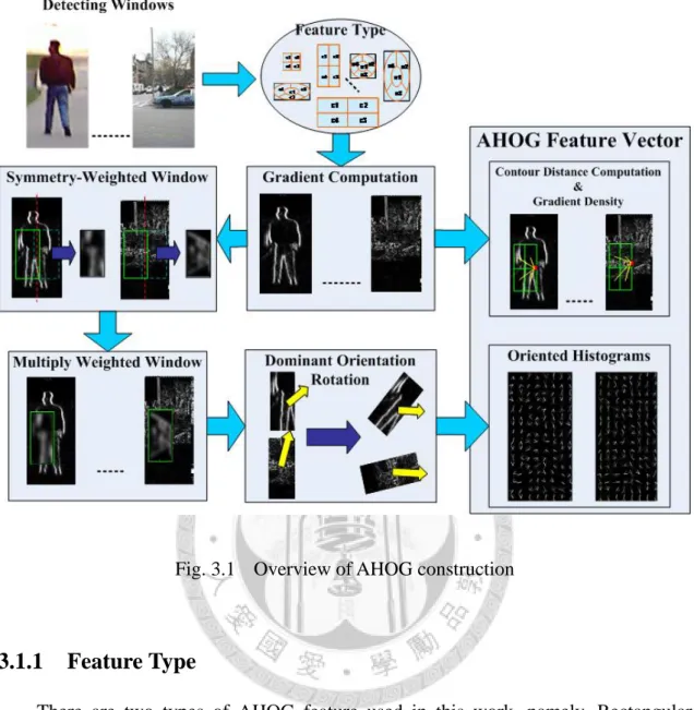
Fig. 3.1 Overview of AHOG construction ...28

Fig. 3.2 AHOG feature structure...29

Fig. 3.3 AHOG feature type...30

Fig. 3.4 Illustration of aspect ratio and block location interval ...31

Fig. 3.5 Illustration of gradient at (x, y) ...31

Fig. 3.6 Symmetry exists in humans. ...32

Fig. 3.7 Comparison of symmetric weighted and Gaussian weighted (intensity of block means the weighted values). (a) Feature block. (b) Symmetry weight. (c) Gaussian weight. ...32

Fig. 3.8 Flow of computing symmetry weighted window. ...35

Fig. 3.9 The symmetry weighted values in longitudinal and lateral views...35

Fig. 3.10 Weighted gradient image ...36

Fig. 3.11 Repetitive patterns ...37

(9)

Fig. 3.12 Contour distance ...38

Fig. 3.13 Limb variation ...39

Fig. 3.14 Orientation histograms ...40

Fig. 3.15 Flow of dominant orientation rotation...41

Fig. 3.16 Quantized orientation histograms ...42

Fig. 3.17 Visualization of orientation histograms ...42

Fig. 3.18 Potential detecting windows ...44

Fig. 4.1 False detected candidates...47

Fig. 4.2 Connected component ...48

Fig. 4.3 Best-fit ellipse estimation ...50

Fig. 5.1 Camera configuration ...52

Fig. 5.2 Human Databases ...53

Fig. 5.3 Number of weak classifier of each stage ...54

Fig. 5.4 Rejection rate of each stage ...54

Fig. 5.5 Intensity histograms of feature block ...56

Fig. 5.6 Visualizing the selected HOG and AHOG. ...57

Fig. 5.7 ROC curve ...58

Fig. 5.8 Experiment results ...62

(10)

LIST OF TABLES

Table 1.1 Traffic Accidents in Taiwan Area (Source: National Police Agency, Ministry of the Interior of R.O.C.) ...2 Table 5.1 Platform details...52 Table 5.2 Performance of each video. ...59

(11)

Chapter 1 Introduction

Nowadays, computers in various forms appear almost everywhere in our daily lives, and they perform tasks of repetitively computing a huge amount of data, more efficiently and more accurately than humans. It is natural to try to extend the computing capabilities to do more intelligent tasks such as interpretation of visual scene or speech, logical inference, and reasoning. Let’s take the human visual system as an example.

There are thousands of objects ranging from man made classes, like cars, bicycles, buildings, windows, to natural ones, like dogs, cows, trees, leaves, mountains and humans. Any one of these has large intra-class variation. For example “car” is used to denote the vehicles which have four wheels. Many various sub-categories are included in this class like a sedan, roadster, jeep or trunk. However, different sizes, colors, or viewpoints, will not affect the human’s capability to recognize vehicles. In the same way we have ability to find people even though they are under widely varied conditions, such as with difficult clothes, accessories, poses, partial occlusions, levels of illumination or kinds of background clutter. Currently, the capability of computers is still far behind that of humans when performing such tasks. Thus, one objective of this research is to enable computers to interpret human objects in the images or videos. In fact, many applications will follow this sharp ability, for example, human computer interaction, autonomous robotics, automatic analysis of digital media content, and pedestrian warning system.

In this chapter, we introduce the problem of object detection, especially in detecting people. We start in Sect. 1.1 with the motivation of human detection, and then in Sect. 1.2 we discuss objectives and some difficulties of this work. We also review some researches related to this problem and summarizes the contributions of them in

(12)

Sect 1.3. Finally, the outline of this thesis is given in Sect 1.4.

1.1 Motivation

Understanding human activity from a video is an active research in the field of computer vision in the last few years and it has applications in various fields, such as surveillance, intelligent user interface, and pedestrian warning system for intelligent vehicle. Before recognizing the human activity, we have to know where the humans are.

Once the human is detected, the system can do further processing to analyze the human activity. For an example of pedestrian safety, the most serious problems that lead to traffic accidents are often due to carelessness of the driver on the pedestrian. Actually, during recent five years, there are about 14,000 people who were killed out of the 13,300 fatal accidents in Taiwan, referring to Table 1.1. Thus, a pedestrian warning system based on an advanced human detection mechanism is needed to reduce the number of accidents caused by unawareness, since it constantly reminds the driver to take care of all the relevant traffic participants like pedestrians or motorbike riders.

Year Number of Fatal Accidents Killed (Persons) Injured (Persons)

2003 2,572 2,718 1,262

2004 2,502 2,634 1,248

2005 2,767 2,894 1,383

2006 2,999 3,140 1,301

2007 2,463 2,573 1,006

Total 13,303 13,959 6,200

Table 1.1 Traffic Accidents in Taiwan Area

(Source: National Police Agency, Ministry of the Interior of R.O.C.)

(13)

1.2 Challenges of Human Detection

The human category in object detection is probably one of the most difficult cases because it combines the difficulties of dealing with a moving camera, a broad range of deformable object appearances and poses, various types of human clothes, complex backgrounds, and highly varied illumination conditions in the outdoor environments. In the following, we discuss and analyze each difficulty of this problem.

First, the general image formation suppresses 3D depth information of the objects.

Different camera viewpoints slightly changes positions and orientations of the objects in the image. In other words, the object image could have large variations in varied scales.

Thus, a sound object detector has to tackle the problems of changing viewpoints and scales.

Second, unstable illumination and various object colors also affect decision made by the object detector. For example, objects appearing directly under sunlight or trees may affect the target region due to possible blending of tree shadows. A sound object detector must handle the color changes and provide an invariant method to accommodate a broad range of illumination changes.

Third, natural objects usually have high intra-class variations, like mankind.

Because human is an articulated object, its pose generally varies with time. Besides that, human appearances often change with clothes or accessories he or she wears. A reliable object detector must be independent of these variations.

Fourth, complex background varies with time while the camera is non-stationary.

For example, the videos are taken under various setting, such as in outdoor environments in cities or within indoor scenes. Moreover, there are many patterns which repetitively occurr in the background, like the trunks of trees, windows on the wall, and

(14)

streetlamps. These factors in the background may lead to many false detections. In order to alleviate the effects caused by these factors, more strict decision rules are needed, but these strict measures may conflict with the previous challenge. That is, because of the high intra-class variations, the system should loosen the decision rules to reduce the number of missed detection of targets. Therefore, a robust object detector must possess the capability of distinguishing targets from the clutter background.

Fifth, partial occlusions cause further difficulties since parts of the object become invisible and the remaining parts contain insufficient information for subsequent processing.

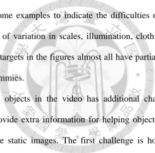
Fig. 1.1 shows some examples to indicate the difficulties of human detection. It includes a wide range of variation in scales, illumination, clothing, pose, appearance, and environment. The targets in the figures almost all have partial occlusions and some targets are even the dummies.

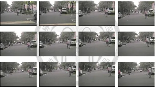
Finally, detecting objects in the video has additional challenges, although the motion feature can provide extra information for helping object detection, the feature becomes useless in the static images. The first challenge is how to remove adverse imaging due to sudden jump of the camera and which usually occurs on the scraggy ground, like pits, drain covers, or tiles. Fig. 1.2 shows image examples taken subjected to unstable shaking of camera while the camera platform crosses the slowdown roadblocks. By observing the sequence of images, we know that the height of object with respect to image coordinate is very unstable in a short time. Another challenge is hard to compute the target’s motion vector very clearly when the velocity of camera is much faster than that of the target sometimes on when the target motion is unobvious and the target is far from the camera. The third challenge is that the problem caused by interlaced process while the camera captures the data. This interlaced process causes

(15)

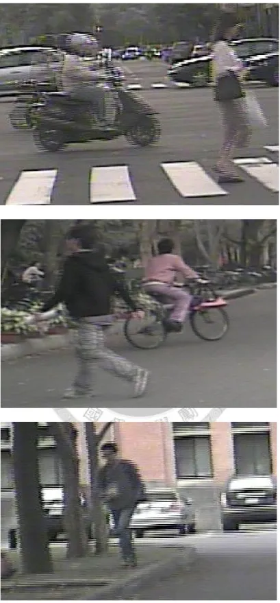
some adverse effects, such as an edge flicker, an interline flicker, and a line crawling, which especially occurs when object’s moving direction is different from that of the camera. Fig. 1.3 reveals some adverse effects on images due to the problem with interlaced process on objects’ boundary. These artifacts make the object’s appearance more uncertain as that the object becomes harder to be recognized. For these reasons, a reliable object detector has to use a robust feature set to cope with the above difficulties and to achieve reliable detection.

(16)

Fig. 1.1 Examples include targets with a variety of difficult factors.

Fig. 1.2 Camera moves up and down while crossing the slowdown roadblocks.

(17)

Fig. 1.3 Examples of interlaced problem

(18)

1.3 Related Work

In recent years, these have been widespread interests in studying problems with human detection, and many researches results have been repeated. So far, the proposed various methods can be classified into motion-based type and appearance-based type according to the way the targets are represented.

The motion-based approach observes the human’s motion in human movement through video sequences. The most direct way is to learn the typical motion patterns of human movement. For example, Viola et al. [1] compute the different directions between successive images as human motion patterns, which and then learned by AdaBoost algorithm to obtain a set of decision rules for detecting people. Little and Boyd [2] take the optical flow of two successive images as feature points of the human’s motion and analyze the motion periodicity to confirm the existence of moving human.

In [3], Heisele and Woehler extract the corresponding regions of two successive images through region tracking technique and use the Time-Delay Neural Network to detect the changing frequency of the width of the observing region to achieve human detection.

Through observation of image sequences, it is known that the gait of human’s walking is a distinct feature as suggested by Wang et al.[4]. Therefore, some researches put this periodic motion feature – gait – in use. In Cunado et al.[5], there are detailed descriptions and definitions about human gaits. They propose a pendulum model to describe the process of human’s walking. Curio et al. [6] combine texture and contour information extracted from video sequences along with motion patterns of humans’

gaits. Niyogi and Adelson [7] compute the differences of human silhouette in XYT-axis frame to obtain the gait pattern for gait detection. Based on the results in [8], Yang Ran et al. [9, 10] proposed a Twin-Pendulum Model to represent the gait of walking people.

(19)

They use image processing techniques to find the maximal and minimal angles between two limbs as the periodical motion features.

On the other hand, the appearance-based approach uses a set of appearance features of static human image to detect the existence of the target. This category uses low-level features to represent the possible human looks and apply standard pattern recognition process to find the corresponding appearance for detecting humans. Broggi et al. [11] use vertical symmetry properties of human shape to detect the position and the size of a human. Hayfron et al. [12] detect the humans by analyzing the symmetry information in spatio-temporal domain. Wu and Yu [13] proposed a two-layer statistical field model combining the Boltzman model and Markov model to describe the features of the non-rigid human shape. Their approach still works even when some parts of the human body are self occluded. Besides, the two-layer statistical field model flexibly describes the observations from the image. Another solution of appearance-based approach is based on template matching, which constructs the human templates from different viewing angles and poses and detects the humans by comparing the appearance feature with the constructed templates. For representing human appearance, Gavrila et al. [14, 15] and Liu et al. [16] characterize the human shape by silhouette or edge image and then transfer them into distance transformed images. But the above approaches fail to detect partially occluded humans due to the fact that they only take the global features – entire human shape. Thus, many researches detect humans via detection of each part of the human body and analysis of the relations among them to reconstruct the human shape. An example is by Mohan et al. [17], where they use an Adaptive Combination of Classifiers (ACC) to detect all kinds of body parts and integrate all part-classifiers to classify the humans. For more examples, Ramanan et al. [18] propose a pose model based on the human body parts, and they use a set of human poses to lock

(20)

the human candidates who are then tracked through detecting of the model generated from each image. Leibe et al. [19] propose an Implicit Shape Model (ISM) to model the relations between body parts and body centroid, and then apply a voting process to determine the human’s position. In order to tackle the problem with translation, scale, and orientation, many low-level features are proposed as well. For example, Oren et al.

[20] propose Haar vertical and horizontal wavelets to compute the intensity variations of the target’s appearance. The results by Wu and Nevatia [21] and by Sabzmeydani and Mori [22] use the edgelets and shapelets as the local features to describe the human shape. The edgelet feature is constructed by comparing the similarity between images and predefined edgelet templates, which differ in number of edge, orientations, single or pair. Similar to edgelet feature, shapelet feature is a set of edgelet feature. In another word, shapelet feature is a piece of shape. In addition, the work by N. Dalal et al.[23] is the first one which uses the Histograms of Oriented Gradients (HOG) to represent the features of people and becomes the performance benchmark in the field of human detection. Based on [23], Zhu et al.[24] use variable feature types to describe humans more flexibly and also improve the processing time by changing single complex classifier into a cascaded set of simple classifiers. Wang et al. [25] rotate each HOG feature according to its orientation to achieve the invariance of geometrical translation and rotation.

Recently, many automobile manufacturers including Toyota, DaimlerChrysler, BMW, Volvo, Honda, etc…have spent many efforts on transferring the technology of human detection to develop a pedestrian warning system on an intelligent vehicle. For example, the Mobileye [26] has developed maturity products that are equipped on advanced vehicles, but the prices of the entire system are still expensive because the system includes various types of sensors, like radar, laser, and camera. The related

(21)

information and materials of their work can be found on their respective web sites.

1.4 Objective

This thesis research aims at the problem of human detection in visual images and videos. In particular, we address the topic as how to constructing a human detector from a view point of computer vision, where the detector is used to search through the input images or videos for humans and their locations. For being more precise, we can see a human detector as a combination of two parts: a feature extraction algorithm which encodes image regions or parts of videos as feature vector, and a detector which uses the computed feature vector to determine whether the object is human or non-human. We give the formal problem definition in the Section 2.1.

1.5 Organization

This chapter introduces a brief background of object detection in computer vision, gives the reason why we need to detect humans, and discusses what difficulties in human detection. We also introduce the state-of-the-art results in the field and give the summaries of these pieces of work. The remaining chapters are organized as follows:

Chapter 2 describes the problem of human detection and some preliminary knowledge about machine learning. In final section, we give the overview of our approach.

Chapter 3 describes the computation of Augmented Histograms of Oriented Gradients (AHOG) feature vector in detail. It discusses the human shape properties and also presents the steps of training and detection.

Chapter 4 presents the approximation of human candidates detected from

(22)

classifier mentioned in Chapter 3. It describes the details of calculating the features of a human shape, such as connected components and moments.

Chapter 5 gives the details of experiment and also introduces the benchmark human databases. The performance and the discussion are presented in the final section.

Chapter 6 concludes the salient features of our approach and provides a discussion of the advantages and the limitations of the work. It also suggests some directions for future work in this research.

(23)

Chapter 2 Preliminaries

This chapter states with the mathematical definition of human detection problem, and them introduces preliminary knowledge about some relevant learning algorithms.

Specially, support Vector Machine (SVM) and AdaBoost algorithm are used in the training process in this research work and their details are given in sections 2.2 and 2.3.

In section 2.4, we provide an approach overview of the proposed approach and describe the relations between different functions. Finally, the contributions of this thesis are summarized in section 2.5.

2.1 Problem Definition

The problem of human detection using a monocular camera can be described as follows. Given the currently observed image frame, the objective is to estimate a collection of parameters that encode the positions of exactly N humans in each image.

Here, the location of each human is encoded by a set of ellipse parameters, namely, (xc, yc) being centroid of ellipse, θ being its orientation, and a and b are lengths of the major and minor axes, respectively. In order to determine the parameters {xc, yc, θ, a, b}, a detecting window W is first used to scan the entire image and is then further classified as human or non-human window by a classifier H(.), that is ,

. ( ) {human, non human}

H W ∈ −

We adopt the AdaBoost algorithm [27] to construct the classifier H(.) by selecting a set of K discriminative features {fi | i=1,…,K} and their associated weak classifiers {hi | i=1,…,K}. Each weak classifier is of the form:

1 if ( ) i

( )

0 otherw ise

i i i

i i

p f p

h f ⎧ ϕ ^< τ

= ⎨⎩ (2.1)

(24)

where ϕ(.) is a mapping function that maps a feature to a real value, ( ,

i )

τ ∈ −∞ ∞ is the classification threshold, and pi= ± 1 indicates the direction of

inequality sign. Then, the classifier H(.) can be further formulated as follows.

1 1

human ( ) 1

( ) 2

non human otherwise

K K

i i i i

i i

h f c

H W α α

= =

⎧ ≥ +

= ⎨⎪

⎪ −

⎩

∑ ∑

_(2.2)

where αi is the selected weight of the weak classifier hi, which is inversly proportional to the error rate computed by AdaBoost algorithm, and c is a constant for adjusting the thresholds to meet the need of the desired detecting criteria.

The following section gives the formal definition and mathematical inference of the Support Vector Machine (SVM) theory and also describes how to use the SVM to construct the weak classifiers h based on the given feature set. Following brief review of SVM, we introduce the main idea of the AdaBoost algorithm in the further section, which specifically goes over the objective and the theory of the AdaBoost and then presents the detail about the steps of selecting discriminative weak classifiers while adopting the AdaBoost algorithm. Besides, for saving the detecting time, how we apply the cascaded AdaBoost algorithm is also described here.

2.2 Support Vector Machine (SVM)

Support Vector Machine (SVM) is a machine learning algorithm proposed by Vapnik [28] based on statistical learning theory, and it is used to perform data classification or regression. SVM has many particular advantages in solving the pattern recognition problems with small number of samples, or being non-linear and high-dimensional, and it also has been used in many practical applications, such as face recognition, 3D object recognition, text categorization, and image classification.

(25)

2.2.1 Objective of SVM

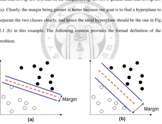
The idea of SVM is that given two sets of classified data, SVM first acquires a classification model after the training process, and then uses the classification model trained by the given data to predict the class to which the non-classified data belong. In simple terms, the objective of SVM is to find a hyperplane to separate data of two sets (i.e. black dots and white dots) in the feature space, referring to Fig. 2.1. Notice that the distance between two parallel solid lines, also called “margin”, in Fig. 2.1 (a) is shorter than that in Fig. 2.1 (b), that is, the margin in Fig. 2.1 (b) is greater than that in Fig. 2.1 (a). Clearly, the margin being greater is better because our goal is to find a hyperplane to separate the two classes clearly, and hence the ideal hyperplane should be the one in Fig.

2.1 (b) in this example. The following context provides the formal definition of the problem.

Fig. 2.1 Comparison of two hyperplanes

(26)

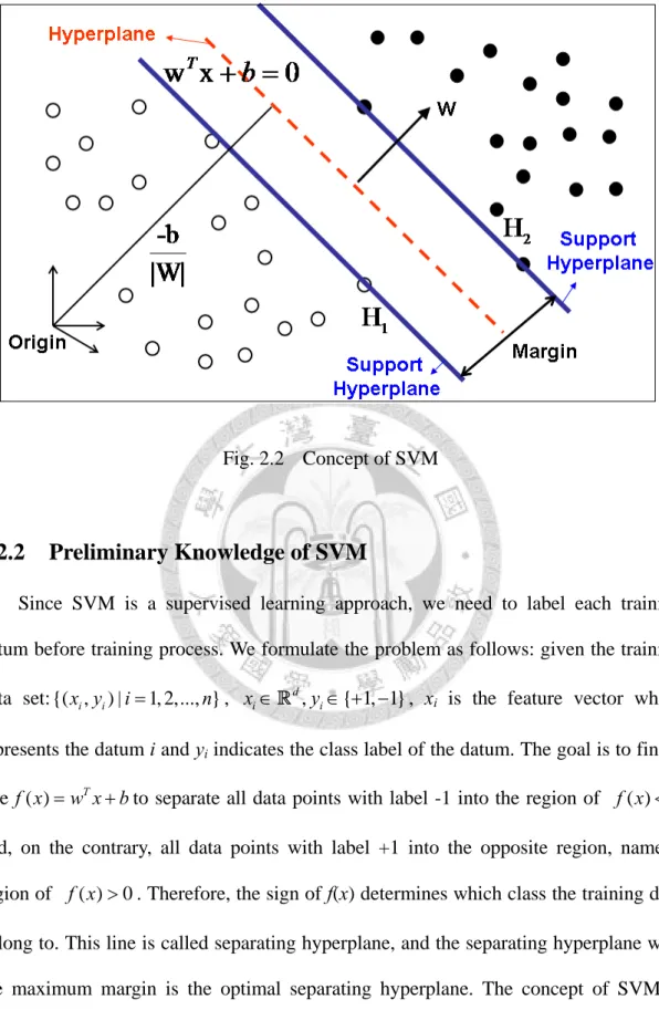
Fig. 2.2 Concept of SVM

2.2.2 Preliminary Knowledge of SVM

Since SVM is a supervised learning approach, we need to label each training datum before training process. We formulate the problem as follows: given the training data set:{( ,x y_i _i) |i=1, 2,..., }n , x_i∈R^d,y_i∈ + −{ 1, 1}, xi is the feature vector which represents the datum i and yi indicates the class label of the datum. The goal is to find a line f x( )=w x^T + bto separate all data points with label -1 into the region of f x( )<0 and, on the contrary, all data points with label +1 into the opposite region, namely, region of . Therefore, the sign of f(x) determines which class the training data belong to. This line is called separating hyperplane, and the separating hyperplane with the maximum margin is the optimal separating hyperplane. The concept of SVM is shown in

( ) 0 f x >

Fig. 2.2, where the support hyperplane (blue line) is the hyperplane which is parallel to separating hyperplane and is closest to the data points. The support

(27)

hyperplanes are formulated as follows:

T

w x b w x b

δ δ + =

+ = − (2.3)

where w is the normal vector of the hyperplane and b is the bias which is the shift distance from the origin. The above equations leads to a over-parameterized problem, that is, supposing we multiply x, b,δ by some arbitrary constant, the equations remain essentially identical, which means that there are infinite sets of parameters x, b,δ that can satisfy the equations. In order to eliminate the uncertainty and simplify the problem, we multiply a constant to scale the parameters and thus the equations can be rewritten as:

1 1

T

w x b w x b

+ =

+ = − (2.4)

Finding the optimal separating hyperplane is equivalent to finding the support hyperplanes with the maximum margin. Thus, we have to maximize the margin = 2/||w||, as to minimize ||w||/2. By recalling the property of the separating hyperplane, can reformulate eq. (2.4) as follows:

1 , if 1 1 , if 1

T i T

i i

w x b y

+ ≤ − ∀ = −i

+ ≥ + ∀ = + (2.5)

( ^T ) 1

i i

y w x + − ≥ (2.6) b 0

To sum up from the discussions given above, we obtain the objective function:

minimize ||w||/2 subjected to y w x_i( ^T _i + − ≥b) 1 0, ∀ , which comprises the primal i problem of SVM. Because the objective function is a quadratic function, which can be solved by Quadratic Programming, the Lagrange Multiplier Method is used to solve the quadratic function with constraints. Specifically, the objective function is transformed to

( , , ) L w bα :

(28)

2 1

( , , ) 1|| || ( ) 1 where 0

2

n T

i i i i

i

L w b α w α y w x b

=

⎡ ⎤

= −

∑

⎣ + − ⎦ ^α ^≥ ^(2.7)

where α is the Lagrange multiplier. To minimize the function L, one applies partial _i differentiation on L w.r.t. w and b, namely,

1

0

n n

i i i i i i

i n

i i i

L w y x w y

w

L y

b

α α

α

=

∂ = − = ⇒ =

∂

∂ = =

∂

∑ ∑

∑

i 1

x

= (2.8)

Therefore, the optimal separating hyperplane:f x( )=w x b^T + can be represented as:

1

( )

T n

i i i i

f x w x b α y x x bT

=

= + =

∑

+ ^(2.9)

Now if α_i ≥0, datum i is on the support hyperplane and it is also called support vector. After obtaining the support vectors, we use them to determine the class to which the datum x belong by following the classification function below:

1

( ) sgn

n T

i i i i

f x α y x

=

⎡ x b⎤

= ⎢⎣

∑

+ ⎥⎦^(2.10)

2.3 AdaBoost Algorithm

The AdaBoost algorithm, first introduced by Freund and Schapire [29], constructs a strong classifier which contains a set of weak classifiers, each of which only needs to have classification rate better than random guess (i.e. error rate < 50%). In computer vision, AdaBoost algorithm is commonly used to find a reliable object detector because it has many advantages: fast and easy to program, only one parameter to tune (the number of iteration), no need to acquire prior knowledge about the weak classifier, and theoretical assurance of obtaining reliable weak hypothesis with sufficient data. Since no prior knowledge is required, the weak classifier can be flexibly combined with any

(29)

means for finding weak hypotheses. Thus, many researches have proposed to fuse various types of feature under the AdaBoost framework and several applications have been accomplished under this framework, such as text categorization, natural language processing, general object detection, and face detection seen nowadays on many commercial digital cameras.

2.3.1 Objective of AdaBoost Algorithm

The objective of AdaBoost algorithm is to find a strong classifier consisting of a set of weak classifiers chosen from a given training data set containing positive and negative data. For each iteration of AdaBoost algorithm, the best weak classifier is chosen according to the error rate that relates to the weight of training data. The main idea of the algorithm is to focus on the incorrectly classified data, called hard examples, by increasing the weight of them to force the algorithm to concentrate on these hard examples. Finally, the selected weak classifiers are combined after their weights are summarized, each is computed by its corresponding error rate w.r.t. training data, so as to construct the final strong classifier.

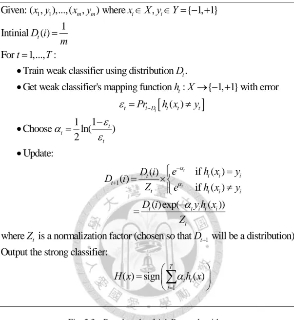
2.3.2 Preliminary Knowledge of AdaBoost Algorithm

AdaBoost is also a supervised learning algorithm for a given train set: {(xi, yi) | i=1,…,m}, where x_i∈{X | instance space}, y_i∈ = − +Y { 1, 1}. The algorithm generates a weak classifier for each iteration, t=1,...,T , and also maintains a distribution of weights over the training set. The distributed weight on the training datum i in iteration t is denoted as . At the beginning, we initialize all weights of the training data by assigning them to an identical value and after each iteration, the weights of incorrectly

t( ) D i

(30)

1}

classified data are increased to make the algorithm choose the best weak classifier according to the weights of the training data at the current iteration. Based on increased of the weights of the hard examples, the algorithm can still maintain the high accuracy with low false positives.

The job of a weak classifier is to determine the label of the training datum X with certain weights. Thus a mapping function that maps a set of real values to real number is . The criterion for selecting a weak classifier is dependent on its error on the training data. The error

: { 1, h Xt → − +

ε of weak classifier t is computed by the following t

equation and the AdaBoost algorithm pseudocode is given in Fig. 2.3

[ ]

~

: ( )

( ) ( )

t

t i i

t i D t i i t

i h x y

Pr h x y D i

ε

≠

= ≠ =

∑

^(2.11)

(31)

1 1

Given: ( , ),...,( , ) where , { 1, 1}

Intinial ( ) 1 For 1,..., :

Train weak classifier using distribution .

Get weak classifier's mapping function : { 1, 1} with erro

m m i i

t

t t

x y x y x X y Y

D i m

t T

D h X

∈ ∈ = − +

=

• • →

[ ]

− +

~

1

r ( )

1 Choose 1 ln( )

2 Update:

if ( ) ( ) ( )

if ( )

t

t i D t t t

t t

t

t i i

t t

t t i

Pr h x y

e h x y

D i D i

Z e h x y

α α

ε α ε

ε

− +

= ≠

• = −

• = × =

≠

1

( )exp( ( ))

where is a normalization factor (chosen so that will be a distribution) Output the strong classifier:

i

t t i t i

t

t t

D i y h x Z

Z D

α

+

⎧⎪ ⎨

⎪⎩

= −

1

( ) sign ( )

T t t t

H x α h x

=

⎛ ⎞

= ⎜ ⎟

⎝ ∑ ⎠

Fig. 2.3 Pseudocode of AdaBoost algorithm

2.3.3 Preliminary Knowledge of Cascaded AdaBoost Algorithm

In order to reduce the classification time cost by the strong classifier learned from the AdaBoost algorithm, we adopt the cascaded AdaBoost algorithm proposed by Viola and Jones [27]. The cascaded AdaBoost algorithm is used for constructing a cascaded weak classifiers which achieves increased classification performance and extremely decreases the computation time. The main idea of the cascaded classifier is to use the simpler classifiers to reject the majority of non-targets before more complex classifiers

(32)

are invoked in order to achieve low false positive rates. Besides that, the detection rate is maintained as well by means of adjusting the threshold of a weak classifier to achieve a false negative rate that is close to zero. The cascaded classifier can be seen as a general decision tree, as shown in Fig. 2.4. A positive result passes all stages of the cascaded classifier and on the contrary negative results are rejected at some stage immediately. The structure of the cascaded classifier reflects that a large number of negative examples are eliminated with very little processing in the previous stages and additional negative examples are eliminated by the subsequent stages. After several stages, the number of examples has been reduced drastically and hence the detecting time has been greatly improved. Different from the AdaBoost algorithm, the training data will change with different stage except at the first iteration. Because of the decision tree-like structure, subsequent classifiers are trained from those training examples which pass all stages up to the current one. Of course, in the further classifiers will face a more difficult task than the previous ones.

Stage 1

Stage 2

Stage n All

examples

Acceptance examples

Rejection examples (Negative)

(Positive)

Fig. 2.4 Cascaded classifier

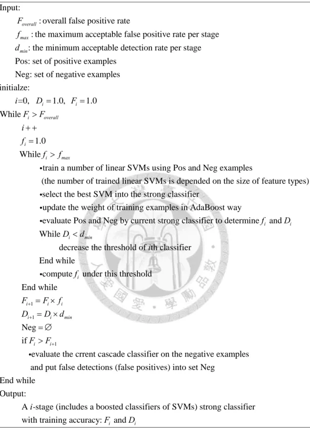
To obtain efficient cascade to meet false positive rate F and detection rate D, the optimal way is to minimize the expected number of features evaluated. Since this

(33)

optimization is extremely difficult, in practice, a simple framework is to choose the maximum acceptable false positive rate and the minimum acceptable detection rate per stage. Each stage is trained by adding weak classifiers until the required detection rate and false positive rates are met. These rates are measured by testing the classifier on a validation set. The final cascaded classifier stops adding stages whenever the overall detection rate and the false positive rate meet the requirement. The detailed pseudocode of the cascaded AdaBoost algorithm is given in Fig. 2.5.

(34)

Input:

: overall false positive rate

: the maximum acceptable false positive rate per stage : the minimum acceptable detection rate per stage Pos: set of positi

overall

max min

F f d

ve examples Neg: set of negative examples initialze:

=0, 1.0, 1.0 While

1.0 While

train a number of linear SV

i i

i overall

i

i max

i D F

F F

i f

f f

= =

>

+ +

=

>

i Ms using Pos and Neg examples

(the number of trained linear SVMs is depended on the size of feature types) select the best SVM into the strong classifier

i

update the weight of training examples in AdaBoost way

evaluate Pos and Neg by current strong classifier to determine and While

i i

i min

f D

D <d i

i

1 1

decrease the threshold of th classifier End while

compute under this threshold End while

N

i

i i i

i i min

i

f

F F f

D D d

+ +

= ×

i

1

eg if

evaluate the crrent cascade classifier on the negative examples and put false detections (false positives) into set Neg

End while Output:

A -

i i

F F

i

+

= ∅

>

i

stage (includes a boosted classifiers of SVMs) strong classifier with training accuracy: and F_i D_i

Fig. 2.5 Pseudocode of cascaded AdaBoost algorithm

(35)

2.4 Approach Overview

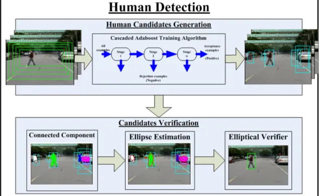
There are two fundamental steps for detecting a human target in our approach. In the beginning, we use grid search over the entire image employing detecting windows with varied scales, and the window’s scale in fact varies with the distance between the camera and the objects, which is also called depth. We represent a detecting window by a set of Augmented Histograms of Oriented Gradients (AHOG) features and generate the AHOG feature vectors as the inputs to the cascaded classifier learned by the cascaded AdaBoost algorithm. The detecting windows passing all stages are considered as the human candidates. The human candidates generated from the classifier need further validation that is accomplished via approximation of the connected components of the human candidates. The moments of the connected component are used to find a fitting ellipse, which is parameterized by size and the orientation. Finally, an ellipse verifier trained by SVM with the given these ellipse parameters is adopted to reject some false candidates for improving the false positive rates. Fig. 2.6 gives the overview of our approach.

2.5 Summary of Contributions

The contributions of this thesis are summarized in the following. The first is the symmetry property of human shape is taken as the weight for each HOG feature. Many noises caused by the complex background may influence measurement of the symmetry property, and thus we add the gradient density to alleviate the noise effects. Besides that, we also transfer the distance between centroid and contour into HOG features to model the geometrical relation between features and centroid. After modeling the relations among features and centroid, the more reliable representing power of a target is

(36)

provided. Moreover, the further human shape approximation by moments of candidate’s connected components increases the detection performance. The difference from the related work is to integrate these human shape properties into HOG features for increasing accuracy while detecting humans. The contributions of our approach are combining human shape properties and HOG to form Augmented HOG features which one then used to represent humans and to verify the candidates by an elliptical verifier to reduce false positives.

Fig. 2.6 Approach overview

(37)

Chapter 3 Human Candidate Detection

This chapter presents the details of generating human candidates. It includes the proposed Augmented Histogram of Oriented Gradient (AHOG) feature set, which describes the feature types, human shape properties, and how to construct an AHOG feature vector. In the next, it gives the description of the training process and analyzes the learned discriminative AHOG features used to illustrate a detecting window. Finally, it presents the method of generating a varied size detecting window for classifying the detected object into a human candidate or a non-human one.

3.1 Augmented Histograms of Oriented Gradients

In this section, we describe two major types of the AHOG encoding method and present the key parameters involved in each type. Section 3.1.1 defines the AHOG feature type, and section 3.1.2 describes the gradient computation. The human shape properties are presented in sections 3.1.3~3.1.5, which includes the symmetry, gradient density, and contour distance. Geometrical rotation invariance and feature vector construction are given at the end of this section. The overview of constructing Augmented Histograms of Oriented Gradients is shown in Fig. 3.1, which gives the flow path between each section.

(38)

Fig. 3.1 Overview of AHOG construction

3.1.1 Feature Type

There are two types of AHOG feature used in this work, namely, Rectangular AHOG (R-AHOG) and Circular AHOG (C-AHOG). Note that R-AHOG feature block uses rectangular grids of cell whereas C-AHOG feature block is divided into grids of cell of log-polar form. The AHOG feature structure is shown in Fig. 3.2. The left one is R-AHOG composed of four grids of cell which divide a feature block evenly. On the contrary, C-AHOG is shown on the right hand side and it is formed with a central cell and three semi-tire shape cells.

R-AHOGs are similar to the SIFT feature as proposed by Lowe [30], but they are actually quite different. SIFT features are computed at a sparse set of scale-invariant key

(39)

points with a Gaussian weighted mask, whereas R-AHOGs are calculated in grids at a certain scale without calling for a Gaussian weighted mask. Moreover, the cell position of the block encodes spatial position relative to the detecting window in the final feature vector. SIFTs are optimized for sparse wide baseline matching, whereas R-AHOGs for dense robust coding of spatial form.

Besides, C-AHOGs are used to encode the shape context into feature vector and allow fine coding of nearby structure to be combined with coarser coding of broader context. The C-AHOG structure has four parameters to denote a layout: center’s position of the block, radius of outer circle, radius of central cell, and expansion angles for subsequent radii.

Fig. 3.2 AHOG feature structure

Besides different types of dividing a block in different forms of cells, we use variable size features for feature selection. Because using multiple scales of blocks and

(40)

cells improves capability of describing an object reported in Dalal’s approach [23], for a 64 × 128 detecting window, we allow the size of all blocks vary from 12 × 12 to 64 × 128. The aspect ratio between block width and block height can be one of the following choices, ( 1 : 1 ), ( 2 : 1 ), and ( 1 : 2 ), for each block. Fig. 3.3 shows the AHOG feature blocks with different aspect ratios, sizes, and the cell order (ci: ith. cell). Some aspect ratios may correspond to some meaningful ratios of human body, and Fig. 3.4(a) gives some examples, say, ( 1 : 1 ) and ( 1 : 2 ), which correspond to human’s head and shoulder and entire human body, respectively. Three interval sizes, 4, 6, 8 pixels of overlapped block locations are used to form a dense grid of overlapping blocks depends on the block size. It means that if the block size is large, the interval should be small in order to well represent the detecting window, and Fig. 3.4(b) illustrates such idea.

Fig. 3.3 AHOG feature type

(41)

Fig. 3.4 Illustration of aspect ratio and block location interval

3.1.2 Gradient Computation

This section describes gradient computation for each pixel. It is accomplished by applying discrete derivative kernels in two directions, horizontal kernel Gh=[-1, 0, 1]

and vertical kernel Gv= [-1, 0 ,1]^T, to obtain the horizontal difference dh(x, y) and vertical difference dv(x, y) at location (x, y). The illustration of gradient computation is given in Fig. 3.5.

( , ) ( , ) ( , ) ( , )

h

v v

d x y f x y G d x y f x y G

= ∗ h

= ∗ (3.1)

Fig. 3.5 Illustration of gradient at (x, y)

(42)

where ﹡denotes convolution operator. Moreover, the gradient magnitude mag(x, y) is calculated by square root of squares sum of horizontal difference and vertical difference, and the orientation of gradient is computed by the following equations:

( , ) _h( , )2 _v( , )

mag x y = d x y +d x y ² (3.2)

1 ( , ) ( , ) tan ( )

( , )

v h

d x y

x y d x y

θ = ⁻ (3.3)

Fig. 3.6 Symmetry exists in humans.

Fig. 3.7 Comparison of symmetric weighted and Gaussian weighted (intensity of block means the weighted values). (a) Feature block. (b) Symmetry weight. (c) Gaussian weight.

(43)

3.1.3 Symmetry

Many researches have shown that representing the human local feature by HOGs is effective in human detection, but it lacks for encoding the beneficial geometric properties, such as symmetry and the relative positions between each part and the human body. We discover that the highly symmetric property exists in human shape no matter whether the human is walking or is standing. Take a walking person for an example; the swinging limbs are at about the same height and are symmetric with respect to human center (other examples are shown in Fig. 3.6 ).

Here, the idea behind our work is to focus on the informative parts of human body rather than the center of each block, and Fig. 3.7 gives an example on the lateral view of a walking human. As can be seen, if the Gaussian weighted window is applied, the feature will only focus on the central part which corresponds to the useless ground plane.

Hence, we take the similarity values of two feature blocks which have symmetric coordinates with respect to the vertical symmetry axis as the new weights used in multiplying the gradient magnitude while constructing the orientation histograms. We assume the symmetry axis is in the vertical center of detecting window. The similarity values are obtained by computing the distance of each pixel of two blocks. In order to be insensitive to slight shift and rotation affection, we not merely think about the similarity of single pixel, but also consider the pixels in the neighborhood instead. The similarity computation flow is shown in Fig. 3.8, and its value similar(x, y) of location (x, y) is measured by the Bhattacharyya distance as follows:

( , ) '( , ) ( , )

similar x y = f x y ×m x y (3.4)

where f’(x, y) is the flipped block which flips all pixels over in the original block and m(x, y) is the mirror block at symmetric coordinates. The symmetry weighted value

(44)

SymWeight(x, y) of location (x, y) is computed by the following equations:

( ', ') ( , )

#( ( , ))

x y N x yk

k

similar x y SymWeight x y

N x y

=

∑

∈

(3.5)

( , ) {( ', ') 0 | ' and ' }

2 2 2

k

k k k

N x y x y Z⁺ x x x y y y

2

= ∈ − ≤ ≤ + − ≤ ≤ +k (3.6)

where Nk(x, y) means the set of pixels in the neighborhood of (x, y), k is the size of neighbors, Z₀⁺ is the set of non-negative integers, and #(Nk(x, y)) is the number of pixels in the neighborhood. Thus, we express the equation of symmetry weighted value in another way as:

( ', ') ( , )

4 2

2

x y N x yk

similar x y SymWeight x y

k

= ∈

⎢ ⎥ +

⎢ ⎥⎣ ⎦

∑

(3.7)

The visualization of symmetry weighted values of a human can be set in two views as shown in Fig. 3.9, which are generated by overlapped grids of smallest cell. The enhanced symmetry part of gradients is given in Fig. 3.10. As can been seen, the discriminative part – shank – is clearly revealed after multiplying the gradients by symmetry weighted window.

(45)

Fig. 3.8 Flow of computing symmetry weighted window.

Fig. 3.9 The symmetry weighted values in longitudinal and lateral views.

(46)

Fig. 3.10 Weighted gradient image

3.1.4 Gradient Density

In practice, there are many repetitive patterns that may cause symmetry computation to fail in the usual scenario. Fig. 3.11 gives some samples of repetitive patterns which occur in the usual scene and these possibly affect the decision of determining the object’s class. To alleviate this affection, combining symmetry and gradient density makes it possible to concentrate on the objects with certain intensity.

Consequently, the gradient density of a block is given by the number of gradient magnitude which is greater than a threshold and then divided by the number of non-zero gradient magnitude. The density value densityblock is given in equation (3.8). Thus,

(47)

combining symmetry and gradient density eases off the influence caused by repetitive patterns in the background. ( #(.) denotes the number of elements )

{ }

( )

{ }

( )

# ( , ) | ( , )

# ( , ) | ( , ) 0

block

x y block mag x y threshold density

x y block mag x y

∈ >

= ∈ ≠ (3.8)

Fig. 3.11 Repetitive patterns

3.1.5 Contour Distance

In order to represent the biologic structural relations among AHOG features, we take the distance between AHOG and human centroid into consideration. Moreover, some human parts might not be symmetric because human could have strange poses, and thus, the symmetric weights of non-symmetric parts will be insignificant, namely, the non-symmetric parts will not be considered afterward. But in practice, non-symmetric parts may have some informative relations between them and human body.

(48)

For the purposes of representing the biological structure relations among AHOG features and keeping the information of non-symmetric parts, we encode the contour distance into AHOG by defining the contour distances as weighted distances between a cell and the centroid of a feature block. Different from [24, 25], we describe the structural relations among AHOGs by adding contour distance into feature vector. On the other hand, our approach is an implicit way of part-based detection under ISM [19]

framework if we use AHOGs to detect human body parts separately. Fig. 3.12 shows the contour distance of a block consists of four distances: cell ci, i=1,…,4, and we calculate the cell distances Disti by the following equations:

( , ) ( )2 ( )

Edist x y = x x− + y y− ² (3.9)

( , )

( , ) ( , )

x y ci

i

mag x y Edist x y

Dist L

∀ ∈

×

=

∑

(3.10)

note that Edist(x, y) means the Euclidean distance between (x, y) and centroid ( , )x y . Each distance is multiplied by the pixel gradient magnitude, mag(x, y), and is normalized to 0~1 by a constant L.

Fig. 3.12 Contour distance

(49)

3.1.6 Dominant Orientation Rotation

Because the highly intra-class variations in the human category, such as swinging limbs at different positions that may confuse human detector (see Fig. 3.13). In order to provide invariance to some affection of the rotational and geometrical variations of a human body, we rotate blocks to its dominant orientation before constructing the orientation histograms. Moreover, the human detector with dominant orientation rotation can use less number of features to represent the same body part even at different positions.

The dominant orientation is determined by the orientation histograms of the feature block. The orientation histograms are constructed from accumulating the weighted gradients (as shown in Fig. 3.10) according to gradient orientation θ. The illustration of constructing orientation histograms is given in Fig. 3.14. The dominant orientation is the angle of the maximum accumulated magnitude (red bar in the figure).

Fig. 3.13 Limb variation

(50)

Fig. 3.14 Orientation histograms

After acquiring the dominant orientation, we rotate the entire block to align the dominant angle with the horizontal, that is, 0°. The histograms of rotated block are shown in Fig. 3.15. From the illustration in Fig. 3.15, two non-rotated histograms of left and right legs are dissimilarity, but after rotating them to their dominant angles, two rotated histograms become more similar. Thus, applying dominant orientation rotation to each feature block not only guarantees invariance to different positions of the body parts but also use the same feature to represent the same body part.

(51)

Fig. 3.15 Flow of dominant orientation rotation

3.1.7 Orientation Histogram Construction

In this section, we describe the way of constructing the AHOG feature vector, which includes gradient density, contour distance, and orientation histograms. First, we calculate four orientation histograms for each cell in a feature block. For time saving, we quantize the orientation into 9 ranges, that is, 40° a range (see Fig. 3.16). Therefore, there are four 9 dimensional orientation histograms within a feature block. The visualization of the four 9-D histograms and entire detecting window with overlapped 9-D histograms are shown in Fig. 3.17. We concatenate the gradient density value, four contour distances, four 9-D orientation histograms to form the final AHOG feature vector for further training and classification.

(52)

Fig. 3.16 Quantized orientation histograms

Fig. 3.17 Visualization of orientation histograms

3.2 Training

Human candidate detection consists of a training process and a detecting process.

Here, we discuss the human candidate training process based on the AHOG features. We construct a cascaded human classifier as mentioned in subsection 2.3.3 with some modifications. Each feature block is described by a 41-D feature vector, which is the

(53)

input vector of SVM as mentioned in subsection 2.2 We use linear SVM provided by libSVM [31] to find the separating hyperplane of weak classifier used in cascaded AdaBoost algorithm. There are more than 14,000 possible AHOG blocks to be evaluated in each stage, but it is very time consuming. So we adopt a sampling approach as suggested by Scholkopf and Smola [32]. They showed that choosing from a small set (5%) of all estimations can obtain a feasible estimation which achieves 95%

performance of the best solution. Thus, we select the best weak classifier from 5% of all kinds of weak classifiers, that is, about 700 weak classifiers trained by linear SVM in each iteration.

3.3 Detection

Human candidates are those detecting windows which pass all stages of the cascaded human classifier as described above. Before classifying a detecting window, we should generate detecting windows with reasonable sizes. The human candidates are determined for further validating step via the candidate verifier. In the following sections, are given the way of classifying the generated potential detecting windows.

3.3.1 Human Potential Location

In this section, we describe how to generate detecting windows with different sizes varied with depths. We adopt the estimation proposed by Hoiem et al. [33] with some modification, which tolerate little errors due to non-flat plane or different human heights.

The height of the detecting window hd relative to depth is given by:

' '

( _d _vanish) _target

d

camera

p p h

h h

− ×

= (3.11)

where pd is the bottom position of the detecting window, pvanish is the position of the