智慧型居家看護影像監控系統(3/3)

行政院國家科學委員會專題研究計畫 成果報告

智慧型居家看護影像監控系統(3/3)

研究成果報告(完整版)

計 畫 類 別 ： 個別型 計 畫 編 號 ： NSC 95-2221-E-002-234- 執 行 期 間 ： 95 年 08 月 01 日至 96 年 10 月 31 日 執 行 單 位 ： 國立臺灣大學電機工程學系暨研究所 計 畫 主 持 人 ： 陳永耀 計畫參與人員： 碩士班研究生-兼任助理：馮孝天、黃璿、劉致廷、江易道 報 告 附 件 ： 出席國際會議研究心得報告及發表論文 處 理 方 式 ： 本計畫可公開查詢

中 華 民 國 97 年 01 月 31 日

行政院國家科學委員會補助專題研究計畫

;

成 果 報 告

□期中進度報告

智慧型居家看護影像監控系統

Intelligent Vision-based Home Care System

計畫類別：

;

個別型計畫 □ 整合型計畫

計畫編號：NSC – 95 – 2221 – E – 002 – 234

執行期間：95 年 8 月 1 日至 96 年 10 月 31 日

計畫主持人：陳永耀 教授 （Chen, Yung-Yaw）

共同主持人：

計畫參與人員：馮孝天、黃璿、劉致廷、江易道

成果報告類型(依經費核定清單規定繳交)：□精簡報告

;

完整報告

本成果報告包括以下應繳交之附件：

□赴國外出差或研習心得報告一份

□赴大陸地區出差或研習心得報告一份

□出席國際學術會議心得報告及發表之論文各一份

□國際合作研究計畫國外研究報告書一份，

處理方式：除產學合作研究計畫、提升產業技術及人才培育研究計畫、

列管計畫及下列情形者外，得立即公開查詢

;

涉及專利或其他智慧財產權，□一年□二年後可公開查詢

執行單位：國立台灣大學 電機工程系(所)

中 華 民 國 九 十七 年 一 月 三 十一 日

Abstract

Intelligent video surveillance system is discussed for years and applied in many areas, like home care systems, security in the public place and so on. Due to this technique development, it can lower down the product cost and decrease the error judgment by human.

In this NSC project, we focused on the home care system which can analyze the human activities automatically. As the growing number of the elder population, more and more people cannot take care of their parents or the elderly all the time. There is definitely a demand to build a system with the ability to watch the elderly and alarm people when they have abnormal behaviors, such as falling down to the ground. In our concept we first want to recognize the human postures, so we set a CCD camera to grab the image containing the elderly and environment. And then we separate the person from the environment using the background subtraction method. After the object is subtracted, some parameters from the silhouette will be extracted and viewed as the input of our classification system. As for the classification system, we use the adaptive fuzzy rule-based system. It can generate the fuzzy rules automatically according to the feature parameters we extract, and give a good performance in classifying the postures.

Keywords: Human Activities, Background Subtraction, Adaptive Fuzzy-Rule Based Classified System

中文摘要

智慧型監控系統在未來的科學研究領域當中，將會是一個值得令人討論的技術。其應 用層面相當之廣泛，不管在居家看護、公共場所安全檢測…等，經由這類的技術發展，不 僅可以降低成本還可以進而改善人為疏失的問題。 在本國科會計劃當中，將會著重在居家看護系統分析與建立的部分。而在居家看護當 中我門所關切的是人類動作行為異常的判斷，也就是說，隨著老年化的社會成長，越來越 多的老年人會待在家中，而當這些老人跌倒甚至發生危險時，我們將會透過這樣的系統提 醒正在遠方工作的兒女，讓他們可以及時的做出解救的動作。而在計劃中，除了異常姿態 的辨識，我們也將辨識一般日常行為中的人體姿態。我們首先利用CCD 攝影機擷取環境影 像，並且利用背景去除的影像處理方式，將移動中的物體擷取出來，並對此物體作簡單的 特徵擷取。藉由得取的這些參數，利用本篇提及的適應性自我學習模糊規則分類系統，產 生模糊規則並且利用這些規則判斷人體姿態。本系統建立了一個常態的模糊規則庫，並將 此應用在人體姿態的分類，最後達成智慧型辨識的能力。 關鍵字：居家看護系統、人體姿態辨識、模糊適應性、模糊規則、背景去除

Table of Contents

Abstract I

中文摘要 II

Table of Contents ... III List of Figures ... V List of Tables ...VII

1 INTRODUCTION ...1

1.1 Motivation ... 1

1.2 Purpose of Research ... 2

1.3 Overview of System Architecture ... 3

2 PRELIMINARIES ...5

2.1 Introduction of Human Activities Identification ... 5

2.2 Modeling of Human Body ... 5

2.2.1 Model Based Approaches ... 6

2.2.2 Non-Model Based Approaches ... 10

2.3 Human Activities Recognition Approaches ... 12

2.3.1 State-Space Approaches ... 12

2.3.2 Template Matching Approaches ... 16

2.3.3 Silhouette Based Method ... 17

3 IMAGE PROCESSING AND FEATURE EXTRACTION ...23

3.1 Moving Object Segmentation ... 24

3.1.1 Block Diagram for Background Subtraction... 24

3.1.2 Auto-Adjust Threshold Algorithm ... 25

3.2 Features Extraction... 27

3.2.1 Definition of Postures ... 28

3.2.2 Definition of Feature Parameters ... 30

4 ADAPTIVE FUZZY RULE-BASED CLASSIFICATION SYSTEMS ...37

4.1 Fuzzy Rule-Based Classification Systems ... 37

4.1.1 Fuzzy Rule Generation Procedure ... 38

4.1.2 Fuzzy reasoning ... 40

4.1.3 Learning Algorithm ... 42

4.2 Apply the AFRBCS in Posture Recognition ... 43

5.1 Hardware Architecture and Environment ... 55

5.2 Experimental Section ... 56

6 DISCUSSIONS AND CONCLUSIONS ...67

Reference List ...68

計畫成果自評 ...73

List of Figures

Figure 1.1 Procedure of human posture recognition. ...3

Figure 1.2 Procedure of human postures recognition. ...4

Figure 2.1 Classification of human motion analysis [3] ...6

Figure 2.2 A stick-figure human model [12] ...7

Figure 2.3 A 2D contour human model [13] ...8

Figure 2.4 A volumetric human model [23] ...10

Figure 2.5 Detecting and Tracking Human “blobs” with The PFINDER System [30] ... 11

Figure2.6 Hidden Markov Model (HMM) ...14

Figure2.7 Example of MEI and MHI [43] ...17

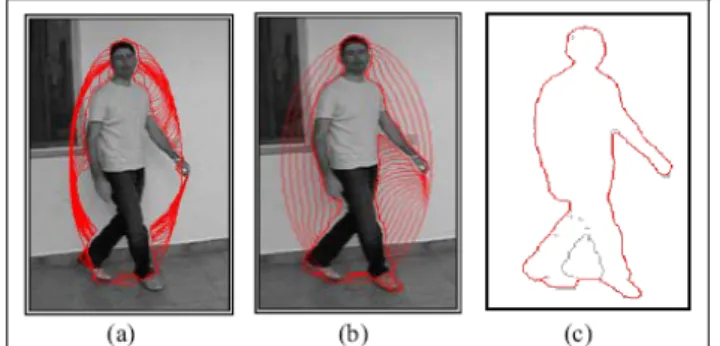
Figure 2.8 Segmentation of a grey-level image through the traditional-snake (a) and GVF-snake (b).Comparison between the final shape of the GVF-snake and the real human shape (c). ...18

Figure 2.9 Left image shows the active contour at the end of the deformation. Right graphics represent the relative Euclidean distance and histogram of radial projections. ...19

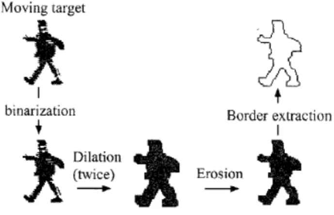
Figure 2.10 Target pre-processing. A moving target region is morphologically dilated (twice) then eroded. Then its border is extracted. ...20

Figure 2.11 The boundary is “unwrapped” as a distance function from the centroid. This function is then smoothed and external points are extracted. ...21

Figure 3.1 Moving object segmentation diagram. ...24

Figure 3.2 (a) Background Image (b) Object Moving Image (c) Segmentation Result ...25

Figure 3.3 Histogram of AD values, x axis is the AD value of total image and y axis is the counter number ...26

Figure 3.6 Stand Postures ...28

Figure 3.8 Kneel Posture ...29

Figure 3.9 Bend Posture ...29

Figure 3.10 Lie Posture ...30

Figure 3.11 Bounding box of the human silhouette and its parameters ...30

Figure 3.12 (a) Segmentation (b) Column Index vs. Counter Numbers ...31

Figure 3.13 Human Hand Spread Plot ...32

Figure 3.14 Modified bounding box of human silhouette ...32

Figure 3.15 Histogram of the human to modify bounding box boundary ...33

Figure 3.16 Definition of neck line plot ...34

Figure 3.17 Parameters of kneel-pose ...35

Figure 3.18 Parameters of Bend-pose ...35

Figure 3.19 All of the Feature Parameters Plot. ...36

Figure 4.1 Plot of membership function of K=5 subsets. ...38

Figure 4.2 Two dimension membership function with don’t-care term ...39

Figure 4.3 Training vectors of five postures distribution in the two dimensions (Xo,Xm) plot. 44 Figure 4.4 Training vectors of five postures distribution in the two dimensions (Xo,Xk) plot. .45 Figure 4.5 Training Vectors of Five Postures Distribution in The 2-D (Xm,Xb) Plot. ...45

Figure 4.6 AFRCS Architecture ...51

Figure 4.7 Standing Training Patterns Images. ...52

Figure 4.8 Sitting Training Patterns Images ...52

Figure 4.9 Lying Training Patterns Images ...53

Figure 4.10 Kneeling Training Patterns Images ...53

Figure 4.11 Bending Training Patterns Images ...53

Figure 5.1 General Postures Recognition Demo Images ...61

List of Tables

Table 4.1 Generating Rules Index Form. ... 47

Table 4.2 Training Patterns for Stand Postures ... 48

Table 4.3 Rules for Recognizing Standing Postures (the first 15 terms). ... 49

Table 4.4 Each βclass Value of Rule 2060. ... 49

Table 4.5 Five postures and its corresponding feature parameters. ... 50

Table 4.6 Training Vectors vs. max( ( )*μ xp CFclass) Values. ... 51

Table 5.1 List of experiment equipment. ... 55

1 INTRODUCTION

1.1 Motivation

The concept of e-home is developed for years, and it involves many aspects of technology. The main goal for an e-home system is always to find an automatic control mechanism that involves watching if there exist some dangers in the home environment and switching on the power of the electric equipments before people coming home and so on. There are many researches in solving these problems, in our research we will focus on the real time intelligent video surveillance systems aspect.

Intelligent video surveillance systems have been mentioned in recent years. We can find many applications in many areas such as airports monitoring systems, home care systems, bank monitoring systems…etc. Especially in home care systems, it is more important in this time as the growing numbers of the elder people. As we introduce before the development of video surveillance systems is so fast cause of that we do not need a lot of security personnel to monitor the human actions. Computer vision is usually used in this kind of intelligent video surveillance systems. It is convenient cause of the information of human body is gathered by using the image processing method without touching or putting the sensor directly on the human body.

As the growth of the elder people, the elderly have more and more time to stay at home without the children’s care. The fast solution is to hire a person nursing beside, but it always has the cost problem. As we know that the cost of the consuming electronics in this time is cheaper and cheaper, to establish a system with some simple electrical products is more convenient and cost down. That is people just need to buy a display and set it up on its own office. Then the parents living situations will be transferred to the display and tell what if there happens some

dangerous.

The home care systems are expected to provide the functions that can monitoring the people inside the house and alarm the watcher when people in some dangerous situations. To give more applications even the human postures can be classified is also needed added. In our approach we want to establish a simple system with a PC and a CCD camera only to get the goal. More application it may be used in the other regions such as the robotics or some artificial science.

1.2 Purpose of Research

In the human action recognition part there are many tasks that are hard to solve. There are two main problems, one is the image processing part and the other is how to define the human action.

In discussing the image processing, the images shot by CCD camera are usual including the moving object and the background. So how to subtract the object we want is a main task dealing with in our system. After getting the object the human action is defined in what descriptions is the next problem. As for the human action there are many words expressed in the similar way like action, behavior, motion, gesture, posture, deed, and movement. For simply dividing, one is the individual static frames like gesture and postures, and the other is continuous dynamic frames like action and behavior.

Our research provides a solution to establish a home care system with the images processing and human action recognition. The image processing part will use a easy concept of background subtraction to complete, and the human action recognition here is focus on the static frame discussion. That is we mainly discuss on the postures recognition parts. The postures part is also can be view as the basic of the human behavior recognition, as you can recognize the human postures the human behavior will be more easily defined.

1.3 Overview of System Architecture

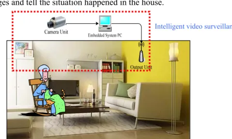
As mentioned before for the easy setup, in our system a camera and a PC are needed and show as figure 1.1. In figure it shows the whole system architecture, the CCD camera is fixed in the corner of the indoor environment and using the image grabbing card to get images, and a PC will process the images and tell the situation happened in the house.

Figure 1.1 Procedure of human posture recognition.

The procedure of imaging processing subtracts the human silhouette from the background image. The silhouette helps us to define the human parameters for the next postures recognition procedure. Of course the parameters we get from the silhouette are usually some characteristic of the human postures. In the postures recognition, it can use the figure 1.2 to explain how it works precisely.

Figure 1.2 Procedure of human postures recognition.

In figure 1.2, the vectors Xp are composed of the parameters we get from the procedure before, and they are viewed as the systems input. In the adaptive fuzzy rule based classified system, it is based on the original fuzzy rule based method with a little change in the generating fuzzy rules. The detail will be introduced in the following sections.

2 PRELIMINARIES

2.1 Introduction of Human Activities Identification

Human activities identification is a quite challenge topic in many kinds of respects. It is complicated in that it can be divided into motion estimation, behavior understanding, and postures recognition. As the various applications of the identification of human activities such as video surveillance, artificial intelligence, medical diagnosis and so on, it is more and more discussed in the computer vision science. In analyzing this problem it usually can be separated from the processing procedure parts. That is in the high level processing tasks usually deal with the body modeling and the whole action identification. As for the low level processing part, they are usually taking the video tracking, segmentation, and pose recovery.

In other words before discussing the problem we need to figure out how the different processing parts works. So in this chapter, section 2.2 will show how to model the human body in two kind of respects, one is based on the pre-build modeling based method to recover a human model and the other is build a human model without pre-model. The section 2.3 will show the key method in modifying the human actions including the HMM method, template matching method and so on. Finally we will give a summary in section 2.4 for the method introduced in this chapter.

2.2 Modeling of Human Body

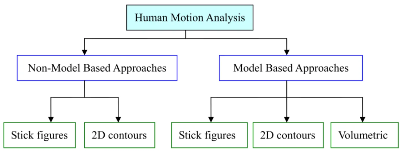
Human motion analysis usually includes human body part segmentation and the recovery of 3D structure from the 2D projections in an image sequence. There are two typical approaches related motion analysis. One is model based method and the other is non-model based approach.

The difference between the two methodologies is in the process of establishing feature correspondence between consecutive frames. Methods which assume a priori shape models match the 2D image sequences to the model data. Feature correspondence is automatically achieved once matching between the image and the model data is established. As no a priori shape models are available, correspondence between successive frames is based upon prediction or estimation of features related to position, velocity, shape, texture, and shape. Conventionally, the representation of human body maybe uses the stick figures, 2D contours, or volumetric model. Section 2.2.1 and 2.2.2 would respectively discuss model based and non-model based approaches. Figure 2.1 shows the classification of human motion analysis.

Figure 2.1 Classification of human motion analysis [3]

2.2.1 Model Based Approaches

Model-based approaches build the body representation by fitting to the image data the predefined parameter values of a parametric body model. This approach can efficiently integrate shape knowledge and visual input, and are better for high-level identification of complicated motions. However, model-based approaches usually require additional processing steps of model selection and parameter estimation to fit the model to a given visual input. Addition of a new

Human Motion Analysis

Non-Model Based Approaches Model Based Approaches

activity or motion may require significant complexity to model-based techniques. In model-based approaches, the fitting process involves either an optimization scheme such as the least square method of Gavrila and Davis [10] or a stochastic sampling scheme such as the particle filtering method by Isard and Blake [11].

In general, human bodies could be represented as stick figures, 2D contours, or volumetric models. Thus, body segments can be approximated as lines, 2D ribbons, and elliptical cylinders, accordingly. Bharatkumar et al. [29] used stick figures to model the lower limbs of the moving human body. They aimed at constructing a general model for gait analysis in human walking. Chen and Lee [12] recovered the 3D configuration of a moving subject according to its projected 2D image. Their model used 17 line segments and 14 joints to represent the features of the head, torso, hip, arms, and legs. The model is shown in figure 2.2.

Figure 2.2 A stick-figure human model [12]

Various constraints were imposed for the basic analysis of the gait. The method was computational expensively, as they use the full search to find the possible combinations of 3D

configurations, given the known 2D projection, and required accurate extraction of 2D stick figures.

The pioneer work of O’Rourke and Badler [27] used a volumetric model consisting of 24 rigid segments and 25 joints. The surface of each segment is defined as a collection of overlapping sphere primitives. Sato et al. [28] developed a different approach that treats a moving human as a combination of various blobs of its body parts. Leung and Yang [13] applied a 2D ribbon model to recognize poses of human performing gymnastic movements. The emphasis of their work is to estimate motion solely from the outline of a moving human subject. The system consists of two major processes: extraction of human outline and interpretation of human motion. The 2D ribbon model is comprised of two components, the “basic” body model and the “extended” body model. The basic body model outlines the structural and shape relationships between the body parts, shown in Figure 2.3.

Figure 2.3 A 2D contour human model [13]

The extended model consists of three patterns: the support posture model, the side-view kneeling model, and side horse motion model. A modified edge detection technique was

developed based on the work in Jain and Nagel [22] to generate a compete outline of the moving object images, A spatial-temporal relaxation process was proposed to determine which side of the moving edge belongs to the moving object. Two sets of 2D ribbons on each side of the moving edge, either a part of the body or that of the background, are identified according to their shape changes over time. The body parts are labeled according to the human body model. Then, a description of the body parts and the appropriate body joints is obtained.

Elliptical cylinders are one of the commonly used volumetric models for modeling human forms. Hogg [23] and Rohr [24] used the cylinder model originated by Marr and Nishihara [25], in which the human body is represented by 14 elliptical cylinders. Each cylinder is described by three parameters: the length of the axis and the major and minor axes of the ellipse cross section. The origin of the coordinate system is located at the center of the torso. Hogg attempted to generate 3D descriptions of a human walking by modeling. Hogg [23] presented a computer program (WLKER) which attempted to recover the 3D structure of a walking person. Rohr [26] found the initial pose of the human first and then incremented it from frame to frame. He used the Kalman filter, edge segmentation, and a motion model tuned to the walking image object for a more robust result. He applied eigenvector line fitting to outline the human image, and then fitted the 2D projections into the 3D human model using a distance measure similar to Hogg [23]. Besides, Rohr [26]’s method identified the straight edges for tracking the restricted movement of walking human parallel to the image plane. The representation of volumetric human model is shown in figure 2.4.

Figure 2.4 A volumetric human model [23]

All of these approaches must match each real image frame to the corresponding model, which represents the human body structure at an abstract level. This procedure is itself non-trivial. The complexity of the matching process is governed by the number of model parameters and the efficiency if human body segmentation. When fewer model parameters are used, it is easier to match the feature to the model, but more difficult to extract the feature. For example, the stick figure is the simplest way to represent a human body, and thus it is relatively easier to fit the extracted lines into the corresponding body segments. However, extracting a stick figure from real images needs more care than searching for 2D blobs or 3D volumes.

2.2.2 Non-Model Based Approaches

As no predefined shape models are assumed, heuristic assumptions, which impose constraints on feature correspondence and decreasing search space, are usually used to establish the correspondence of joints between successive frames. The approaches of non-model based human motion analysis are applicable to more diverse situations. However, these approaches are sensitive to noise in general, because they lack any mechanism to distinguish noise from signal in

visual input.

The approaches of non-model based human motion analysis are also called as view-based approaches. They build a body representation in a bottom-up fashion by first detecting appropriate features in an image. The methods do, however, build some sort of model to represent the pose. These pose representations are points, simple shapes, and stick-figures. The pose of the subject may be represented by a set of points and is widely utilized as markers are attached to the subject. Without the markers, the hands and the head may be estimated from the image represented by just three points [30] as figure 2.5. This is a very compact representation which suffices for a variety of applications. By utilizing color segmentation [31] or blob segmentations [30], these three points are usually found.

Figure 2.5 Detecting and Tracking Human “blobs” with The PFINDER System [30]

A subject in an image can be simply represented into some boxes by the boundary of subject [32]. However, the boundary box representation is mainly utilized as an intermediate representation during processing and not as the final representation. Instead, shapes which are more human-like, such as ellipses [33], may be used as a final representation.

features to posture data. In the work proposed by Brand [34], the paths through the 3D state space obtained through training are modeled using an HMM where the states are linear paths modeled by multivariate Gaussians. As in [35] the moments (central) are found by synthesizing various poses. The moments are associated to the HMM. Altogether a sequence of moments is mapped to the most likely sequence of 3D poses. Obviously this approach is either offline or includes a significant time-lag, but it has the ability to resolve ambiguities using hindsight and foresight.

2.3 Human Activities Recognition Approaches

For human activity or behavior recognition, most efforts have been concentrated on using state-space approaches [36] to understand the human motion sequence [37, 38, 39, 40]. Another approach is to use the template matching technique [41, 42, 43] to compare the feature which is extracted from the given image sequence to the pre-stored patterns during the recognition process. There are still some researches in discussing how to get the human feature from the silhouette image, like image skeletonization [5, 29], active contours based [1], and so on.

The approaches which are related to human action recognition will be surveyed and introduced in this section. Besides, the recognition of human behavior is our future desired research. Some approaches of human behavior recognition will be presented below.

2.3.1 State-Space Approaches

Approaches using state-space models define each static posture as a state. These states are connected by certain probabilities. Any motion sequence as a composition of these static poses is considered a tour going through various states. Joint probabilities are computed through these tours, and the maximum value is selected as the criterion for classification of activities [3]. Most

studies using state-space model have applied the methods of ‘Dynamic Time Warping’ (DTW) [33] or ‘Hidden Markov Model’ (HMM) [30].

DTW is a method of sequence comparison used in various applications such as DNA comparison in microbiology, comparison of strings of symbols in signal transmission, and analysis of bird songs and human speech. DTW deals with differences between sequences by operations of deletion-insertion, compression-expansion, and substitution, of subsequences. By defining a metric of how much the sequences differ before and after these operations, DTW classifies the sequences. DTW can also be applied to image sequences. However, DTW lacks the consideration of interactions between nearby subsequences occurring in time. In many actual situations, a sequence has higher correlation between closer subsequences than between distant subsequences [44].

State-space models have been widely used in the recognition of human activities. Hidden Markov Model (HMM) is a finite set of states, each of which is associated with a probability distribution. HMM has been successfully applied in speech recognition [10, 35]. Recently, it has been applied in the research field of image processing and computer vision such as handwritten character recognition, human action recognition [30, 45], sign language recognition, and facial expression identification [12]. The conception of HMM comes from the Markov chain. The most difference between hidden Markov model and Markov chain is that HMM can not acquire the states of event directly. HMM must utilize the observation function to infer the event states indirectly. The observation is a probabilistic function of the state. The basic HMM model can see the Figure 2.6.

Figure2.6 Hidden Markov Model (HMM)

In order to define an HMM completely, following elements are needed.

„ N: the number of states in the posture graph. The model state at time t is denoted as qt , 1≦qt≦ N , 1≦t≦ T.

„ T : length of the observation sequence.

„ S={ Si | 1≦i≦ N }：a set of model-states; if the state is k at time t, it is denoted as qt = Sk . „ M：the number of observation model-states.

„ V={ vi | 1≦i≦ M }：a set of observation model-states.

„ A={a | 1≦i,j≦ N }：a state transition probability distribution, where _ij a =P(q_ij j at n+1 | qi at n ).

„ B={ bj(k) | 1≦j≦ N and 1≦k≦M } : an observed state probability distribution where bj(k)= P(vk at t | qt = Sj ).

„ Π={πi | 1≦i≦ N }: an initial state probability distribution , where πi = P(qj = Sk).

„ λ = (A,B, π) : HMM parameter.

„ O={O1,O2,…,OT} : observable symbol sequence.

The complete parameter set λ of the discrete HMM is represented by vector π and matrices A State 1

and B. In order to accurately describe a real world process such as posture with a HMM, the HMM parameters have to be selected accurately. The parameter selection process is called the HMM training process. This parameter set λ can be used to evaluate the probability P(O | λ), that is to measure the maximum likelihood performance of an output observable symbol sequence [46].

There are three basic problems in HMM design: 1. Evaluation problem

Given the observable symbol sequence O={O1,O2,…,OT} and the HMM parameter set

λ=(A,B, π), how do we efficiently compute the probability P(O| λ) ? 2. Estimation problem

Given the observable symbol sequence O={O1,O2,…,OT} and the HMM parameter set

λ=(A,B, π), how do we choose an optimal corresponding state sequence q = (q ,q , q )_{1 2} L _T ? 3. Training problem

How do we adjust an HMM parameter set λ=(A,B, π) in order to maximize the output probability P(O| λ) of generating the output observable symbol sequence O={O1,O2,…,OT} ?

These problems have had complete and effective theory to solve. Problem 1 utilizes the forward-backward algorithm to reduce computation [49, 50]. Problem 2 uses the Viterbi algorithm to find the state which has a maximal probability at a given time [47, 48]. Problem 3 utilizes the Baum-Welch algorithm to increase training efficiency [46].

A good tutorial for details of HMM is proposed by Rabiner [48]. HMM has been more popular than DTW for dynamic representation of action because of its ability to handle uncertainty in its stochastic framework. For instance, hand motions are classified by HMM [49]. Min et al. [50] used both static representation and dynamic representation for hand gesture recognition. Yang et al. [51] applied HMM to classify human action intent and to learn human skills.

2.3.2 Template Matching Approaches

The template matching approaches analyze the individual frames first and then combine the results. The motion magnitude in each cell is summed, forming a high dimensional feature vector used for recognition. To normalize the duration of the movement, they assume that human motion is periodic and divide the entire sequence into a number of cycles of the activity. Motion in a single cycle is averaged throughout the number of cycles and differentiated into it fixed number of temporal divisions. Finally, activity recognition is processed to use the nearest neighbor algorithm.

In an early research, Herman [52] utilized the template matching of stick-figures of a given frame to analyze different poses of a person. The emotions and actions at a given frame based on the person’s pose are inferred. His stick figure was built by manually locating body parts, and he analyzed individual frames separately, without considering the interrelations between the frames in a sequence. Akita [53] used template matching of silhouette images to recognize different motions of a person in tennis play. Recent work by Bobick and Davis [41], they follows the same vein, but extracts the motion feature differently. They interpret human motion in an image sequence by using motion-energy images (MEI) and motion-history images (MHI). The example can see the figure 2.7. The MEI is binary images containing motion blobs. The motion images in a sequence are calculated via differencing between successive frames and then threshold into binary values. The MEI (E_T(x,y,t)) is combined by these motion images in time and is defined:

1 0 ( , , ) ( , , ) T i E x y t D x y t i τ− = =

_U

− (2.1) where D(x, y, t) is a binary image sequence indicating regions of motion, τ is critical in defining the temporal extent of a movement.

MHI is to represent how motion the image is moving. The each pixel value is proportional to the duration of motion at that position. The MHI (H_τ(x,y,t)) is defined:

if ( , , ) 1 ( , , ) max(0, ( , , 1) 1) otherwise D x y t H x y t H x y t τ τ τ = ⎧ = ⎨ _{− −} ⎩ (2.2)

The MEI can be generated by threshold the MHI above zero. Moment-based featured are extracted from MEI and MHI and employed for recognition using template matching.

Figure2.7 Example of MEI and MHI [43]

2.3.3 Silhouette Based Method

the next activities identifications. It means first the image subtractions for the moving object is all needed to be done. As the silhouette getting the next procedure is divided into some different method. [1] efforts the active contours features to represent the human postures, [2] take the Fourier transform concept to develop an image Fourier descriptor method. It will be introduced one by one.

A. Active Contour Based Method

In the research mentioned, Buccolieri [1] give a method using the active contours as the image features and take this as the NN input to model a systems in recognition the postures. The system architecture consists of five sequential modules that include the moving target detection process, two levels of segmentation process for interested element localization, features extraction of the object shape and a human posture classification system based on the Radial Basis Functions Neural Network. Moving objects are detected by using an adaptive background subtraction method with an automatic background adaptation speed parameter and a new fast Gradient Vector Flow snake algorithm for the elements segmentation is proposed.

The GVF-snake method can separate the object as the figure 2.8, its detail derivation is not mentioned here.

Figure 2.8 Segmentation of a grey-level image through the traditional-snake (a) and GVF-snake (b).Comparison between the final shape of the GVF-snake and the real human shape (c).

In its research, it use the three layers Radial basis function neural network, and as for the input of these system is the Euclidian distance form the snake center that is shown in the figure 2.9. The Euclidian distance is calculated by the equation 2.X expressed as bellow.

Figure 2.9 Left image shows the active contour at the end of the deformation. Right graphics represent the relative Euclidean distance and histogram of radial projections.

2 2 ( ) ( ) 1 i i c i c d = x −x + y −y i= Ln ………. (2.3) 1 1 1 1 , y n n c i c i i i x x y n = n = =

∑

=

∑

……….. (2.4)

Where ( ,y ) x_{c c} means the center of the contours and ( ,y ) x_{c c} is the coordinate of each point

on the contour, and n is the number of the contour points. As the features can be extracted the input is chosen from these data. Although these features are easily evaluated, a high number of them is necessary (depending of the object’s size) and, moreover, they are too sensitive to excess parts (noise and shadow) and to lacking parts.

There is another extension active contours method for the analysis of human motions. [5, 29] take a more deepgoing process to represent a human model. From these, a “star” skeleton is produced. Two motion cues are determined from this skeletonization: body posture, and cyclic motion of skeleton segments. These cues are used to determine human activities such as walking or

running, and even potentially, the target S gait. Unlike other methods, this does not require an a priori human model, or a large number of ‘pixels on target”. Furthermore, it is computationally inexpensive, and thus ideal for real-world video applications such as outdoor video surveillance.

For getting the ‘star’ shape of a tracking human model it is using some image process from segmentation of the moving object and using morphology process like dilation and erosion it shows in the figure 2.10. The figure shows the whole preprocess procedure step by step. The process dilation is first fitting the hole in the original image then using erosion the make the image thinner. Finally grab the contour for the image and finish the pre-process.

Figure 2.10 Target pre-processing. A moving target region is morphologically dilated (twice) then eroded. Then its border is extracted.

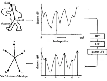
As the pre-process finished, the data process part is then continued. It is shown in the figure 2.11. The figure shows the main procedure in getting the star skeleton, that is first calculate the active contour like before and the take the DFT for the data curve, and by using low pass filter to get the low frequency characteristic. Finally do the inverse DFT can get another smooth curve and find the characteristic point to represent the apex of the star shape. And the whole diagram is shown in the figure 2.11.

Figure 2.11 The boundary is “unwrapped” as a distance function from the centroid. This function is then smoothed and external points are extracted.

As a reason that the star shape is somewhat like our hand and foot, the angle from the shape can be view as the motion analysis key point. Besides the angle of the star apex the period of the skeleton changing is also another human motion analysis property. The system then applies the concept to model a running person motion and the detail here will not to be focused.

B. Fourier Descriptor

In the paper, it assumes that a human silhouette can be extracted from monocular visual input. The idea behind Fourier descriptors is to describe a silhouette by a fixed number n of sample points{( ,y ), ,(x0 0 L xn−1,y )}n−1 on the boundary. Since Fourier descriptors can describe only

a single closed-curve shape, we only sample along the external boundary. Sampling can be done randomly but in practice, equidistant sampling is preferred to make sure the sampling is more uniform. The sample points are transformed into complex

coordinates{z , , z }0 L n−1 with zi = +xi yi* −1 and are further transformed to the frequency

the Fourier coefficients, denoted by{ , ,f0 L fn−1}.

The coefficients with low index contain information on the general form of the shape and the ones with high index contain information on the finer details of the shape. The first coefficient depends only on the position of the shape and setting it to zero makes the representation position invariant. Rotation invariance is obtained by ignoring the phase information and scale invariance is obtained by dividing the magnitude values of all coefficients by the magnitude of the second coefficient f . Since after normalization0 f is always zero and0 f is always one, we have n1 −2

unique coefficients given by:

1 2 1 1 ( f , , fn ) FD f f − = _L (2.5)

This descriptor is a shape signature and can be used as a basis for similarity and for retrieval. When we deal with Fourier descriptors of length n, we actually use only n − 2 coefficients. It is clear that Fourier descriptors describe a shape globally. The finer details are filtered out. Now consider two shapes indexed by Fourier descriptors FD1 and FD2. Since both Fourier descriptors are (n − 2)- dimensional vectors, we can use the Euclidian distance d as a similarity measure between the two shapes:

2 3 0 ( 1 2 ) n j j j d FD FD − = =

∑

− (2.6)

3 IMAGE PROCESSING AND FEATURE

EXTRACTION

A real time man-less monitoring system requires three main process procedures. One is moving object segmentation, one is feature extraction and the final is the smart sensing procedure. The first of all is to subtract the foreground image like the elderly from the background image. Many segmentation techniques have been developed which can be classified into five types：

(1) Temporal Segmentation, (2) Spatial Segmentation,

(3) Spatial-Temporal Segmentation, (4) Motion Estimation Segmentation, (5) Background Subtraction Segmentation.

In our research we use the fifth kind of method to develop our home care system, we will introduce in the next paragraph. As the foreground object has been captured the features characteristic will be extracted from the object. These features will help us in classifying the human motions. At the final stage we use the Adaptive Fuzzy Rule-based Classification method to model the system. The extracted features are the system input vectors and the output is the classified postures. The whole system will be introduced in the next paragraph step by step.

3.1 Moving Object Segmentation

In this plan, the method we applied in moving object segmentation is the background subtraction. Its main concept is to subtract the current frame from the background frame to separate the foreground object. More precisely, we take the difference operation to see the pixel value change from these two frames. So the problem now is to determine the suitable threshold value to separate the foreground and background. In this plan, the histogram method is used to count the difference pixel value and than the threshold value will be decided. More detail will be introduced in the next sections.

3.1.1 Block Diagram for Background Subtraction

Figure 3.1 Moving object segmentation diagram.

In figure 3.1, it shows the segmentation procedure. In this method the main goal is to get the background and foreground image, so at first the CCD camera will automatically take a quick

shot as the background image. Next step it takes the next frame as the foreground image. Then the system will put these two image into auto-adjust threshold algorithm to get the moving object silhouette, i.e. the gray level value between foreground image and background image changing too large to exceed the threshold the output image gray level value will be assigned as 0. In the final we will get a two gray level value image which gray level value is 0 or 255. In figure 3.2, it shows the result of this applied subtract method.

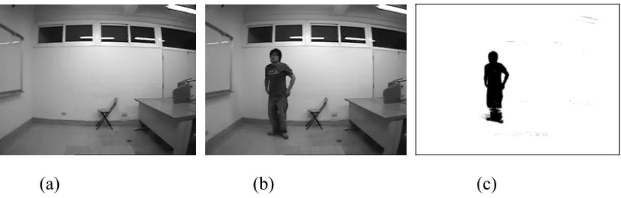
(a) (b) (c)

Figure 3.2 (a) Background Image (b) Object Moving Image (c) Segmentation Result

3.1.2 Auto-Adjust Threshold Algorithm

In this section, the plan will introduce how to decide a good threshold to subtract the object. In the traditional method is determined by the following equations：

( , , ) ( , , ) ( , ) D x y t = F x y t −B x y (3.1) ( , , ) ,if ( , , ) Th ( , , ) 0 ,if ( , , ) Th F x y t D x y t I x y t D x y t ≥ ⎧ = ⎨ _≤ ⎩ (3.2)

In these equations, F(x, y, t) is the pixel value of current frame. B(x, y) is the pixel value of background frame Th is the global threshold value and I(x, y, t) is the segmentation result. D(x, y, t) is the different value between current frame and background frame. So in these two equations above the different threshold value we choose the segmentation will also have different result.

(absolute difference), which is defined as：

( , , ) ( , ) ,where 1 ~ , 1 ~ ij

AD = F i j t −B i j i= dx j= dy (3.3)

It means that we first need to calculate the difference value for each pixel in the capture image, where dx means the resolution of the x dimension of the image and dy means the resolution of the y dimension of the image. After getting the AD value we make a histogram to count this AD value. More precisely, we take each pixel absolute difference from (dx , dy)=(1 , 1) to (dx , dy)=(480 , 640), and assign a row vector, HISTOGRAM(1, 260), to save this value. The length of this row vector is 260 in order to make sure that every pixel’s gray level difference from 0~255 can be saved. For example, if the AD value is 23 we will put one count in the row vector (1, 23), i.e. the value of the HISTOGRAM (1, 23) will be added one. Figure 3.3 shows the histogram plot.

Figure 3.3 Histogram of AD values, x axis is the AD value of total image and y axis is the counter number

As long as we got the histogram, the Rules of Auto-Adjust Threshold will be realized in the next four steps.

1. Find the globally maximal counter number.

2. Search the first locally minimal counter number that is located at right side of globally maximal counter number

c

c

d

d

e

e

3. If the first locally minimal counter number is greater than 100, find the next locally minimal counter number as step 2, otherwise the threshold value is not changed and go to step four 4. Check the index of globally maximal counter number. If the index of global maximum equals

zero, the system will decrease the threshold value. The new threshold value is decided from the point where the SAD variation greater than 150. Otherwise the system does not change the threshold.

The first step assumes the SAD value of background information is lower than foreground information. The second step assumes that there is a border between moving object and background so we find the first local minimum to determine the threshold value. The third step confirmed that the threshold value would not be influenced by false histogram of SAD different value. The fourth step checks the index of globally maximal counter number to monitor the camera noise to apply on different video sequence. If the index of globally maximal counter number equals zero that means the camera noise is very small. If camera noise is small, we will decrease the threshold value to adapt different video sequence.

3.2 Features Extraction

Like the figure 3.2 (c), we got the binary value image i.e. the black pixel gray value is 0 and the white pixel gray value is 1. There are many kind of method in discussing how to extract the human silhouette features, [2] transfer the image into the FD (Fourier descriptor), [1, 5, 29] calculates the image counter called active contour…etc. In the FD method, it is often viewed the 2-D image as the complex plane. Assume the close plane image curve can be got, it take the Fourier transform of this curve, and take the dominate term to represent the image feature, It has the space-invariant characteristic, i.e. the rotation will just differ in phase. But in our goal to

determine a man which is lying is not properly used here because the lying pose is the rotation of the standing pose. The other method, Active Contour, is a kind of contour based method. It first to find out the contour mass center and next to calculate the Euclidean norm between each point and the mass center. Then the distance data will be regard as the feature of the image. Above methods are quite useful for some special situation, but it usually takes time to process this algorithm. So in order to deal with the real time problem, we should take a quick process to find the proper feature. In the next paragraph, the method we use will be discussed.

3.2.1 Definition of Postures

Actually the obvious human pose in this plan is divided into five kinds of postures such as stand, sit, lie, kneel and bend. This section will show this kind of pictures and explain some definition. First we show the stand pose as the figure 3.6.

Figure 3.6 Stand Postures

In the standing poses the hands motions may be an effect of the parameter we define in the next section. So in this plan the most frequent poses people will act are included and discussed. For the purpose to get the real time postures recognition system, besides the standing postures we also consider the other four kinds of postures, such as sit, kneel, bend and lie. They are all shown

as below. In the kneeling and bending postures for the convenience of feature extraction, the side view images are used.

Figure 3.7 Sit Posture

Figure 3.8 Kneel Posture

Figure 3.10 Lie Posture

As getting these postures definition, it is now important to find the different feature expression for these different postures. In the next section the feature extraction methods are discussed.

3.2.2 Definition of Feature Parameters

In fact, in this plan we take the bounding box of human contour, see as the figure 3.11.

Figure 3.11 Bounding box of the human silhouette and its parameters

In the figure 3.11, L1 means the left boundary of the bounding box, R1 means the right boundary of the bounding box, H1 means the upper boundary of the boundary box and F1 means the lower boundary of the bounding box. M1 is calculated by (F1+H1)/2, it means the middle line of the bounding box.

the bounding box will help us to obtain the value we need. Cause of the imperfect of the image segmentation the subtraction image we got usually has some noise. It is shown in figure 3.2 (c), the up-right corner has some noise disturbances. The noise will be viewed as the moving object if we take the boundary by finding the first black pixel we met form left to right, top to down. To solve this problem, we count the black pixel number column by column. As we known the moving object will be assigned the black pixels, and it will occupy the large image space. Again we use the histogram method to record this counter values, figure 3.12 shows the plot. In figure 3.12 the x axis of the lower plot means the x coordinate of the image i.e. it ranges from 1 to 640, and the y axis means the counter numbers of each coordinate. The max counter line here is point out the maximum black pixel counter numbers.

Figure 3.12 (a) Segmentation (b) Column Index vs. Counter Numbers

For finding the outer bounding box we check the black pixel counter numbers from the index of the maximum counter line to the boundary of the image. If the counter numbers of index (i) and (i+1) are not equal to 0, we set the index to be the bounding box boundary. For example in figure 3.12, the index of maximum counter line is 239. From column index 239 to column index 640 the first two zero count numbers are column index 311 and 312. Then the right bounding box boundary, i.e. the parameter R1 in the figure 3.9 is the column index 313. In the same way we can

find the outer bounding box H1, F1 and L1.

In fact, the hand is rising or not will make the bounding box more complicated. It means that when the hand is spread like the figure 3.13, the width of the outer bounding box will become larger than the original width, i.e. the ratio also becomes smaller than the original stand pose ratio. To accurately determine the real human body boundary in this case we should modify the bounding box boundary.

Figure 3.13 Human Hand Spread Plot

Figure 3.14 Modified bounding box of human silhouette

In further discussion, we modify the figure into figure 3.14. The ML1 and MR1 mean the left and right boundary after modifying. The M_Width means the distance between MR1 and ML1. The way we find the modified parameters is also using the same histogram way discussed

before.

As mentioned before, we take the figure 3.15 for the example. We take some mark for the figure 3.12 (b) and it becomes figure 3.15. The symbol B is the main body part of human, symbol A and symbol C are the hand part. It can be obviously found from the figure 3.12 (a) that the black pixel numbers of hand parts are much smaller than the body part, so the boundary of part A and part B is chosen by this concept.

First, after finding the maximum counter numbers of part B, we move to the right part to get the counter numbers of each column. As the process going we pick the column index as the boundary of part B and part C if the counter numbers of the right part divide by the maximum counter numbers is larger than the threshold value. The boundary of part A and part B is also chosen as the same way. It can be seen as the figure, at column index 280 the counter numbers suddenly drop to a small value so we take the 280 to boundary of the modified bounding box.

Figure 3.15 Histogram of the human to modify bounding box boundary

Once again the hand effect is not only in spreading out case, but the raising effect. It means that if the hand is rising over the head the ratio of width-length will be lager than the original case. By solving this kind of problem we take a quick process to define the head line it is shown below. The symbol of N1 in the plot indicates the line which is modified as the neck line. The definition of the line index is calculated by dividing the upper bounding box into three part and we take the 1/3 length for its coordinate. M_Height here represents the length form N1 to F1.

Figure 3.16 Definition of neck line plot

In the next paragraph the two postures, kneel and bend will be discussed. Cause of the specialty of these two postures, that is the length-width ratio of these two postures are easily confused with the sit postures, it is necessary for finding another proper parameters.

The main concepts of our feature extraction are based on the shape method. That is the formation of the postures shape is a kind of index to point out the different postures. Take the kneel postures for example, that is show a below in figure 3.17. In the figure the symbol KN_1 means the parameter to define the kneel-pose line, and the BN_1 means the parameter to define the bend-pose line. More concisely, the other two parameters are defined to calculate the features. The line index of KN_1 is found by finding the maximum black pixel numbers from the half line of lower bounding box to the bottom line of the lower bounding box. It can be drawn as the fig. 3.17 shown. The meaning of BN_1 line is also very clear seen as the fig. 3.18. In the bend-pose, the number of black pixels in the line BN_1 are obviously large than others. For the quick process procedure the line of BN_1 are chosen by take the half of the upper bounding box. For recoding the two parameters we use the symbol of Pixel(BN_1) and Pixel(KN_1) to stand for the pixel numbers of the KN_1 line and BN_1 line.

Figure 3.17 Parameters of kneel-pose

Figure 3.18 Parameters of Bend-pose

1. _Original length−width ratio_ =(Height Width/ )≡ x_o

2. Modify length_ −width ratio_ (1) (= Height M/ _Width)≡xm1

3. Modify length_ −width ratio_ (2) (= M _Height M/ _Width)≡x_m2

4. _Kneel ratio=(Pixel KN( _1) /Pixel BN( _1))= xk 5. _Bend ratio=(Pixel BN( _1) /Pixel KN( _1))≡ x_b

Figure 3.19 All of the Feature Parameters Plot.

By summing all above up, we can derive five main feature parameters for our classifier system. It can be summarized as the five equations shown below. Figure 3.19 shows the parameters plot for the system. All the five parameters can be derived from the plot, ant the plot in other words is the summary of all the plots shown before. So in our processing, every image taken by the CCD camera will be through the image subtraction and feature extraction. Then we can get the feature extraction vector which has the five components, like ( ,x= x xo m1,xm2, , ) x xk b represents.

4 ADAPTIVE FUZZY RULE-BASED

CLASSIFICATION SYSTEMS

This paper proposes an adaptive method to construct a fuzzy rule-based classification system with high performance for pattern classification problems. The proposed method consists of two procedures: an error correction-based learning procedure and an additional learning procedure. The error correction-based learning procedure adjusts the grade of certainty of each fuzzy rule by its classification performance. That is, when a pattern is misclassified by a particular fuzzy rule, the grade of certainty of that rule is decreased. On the contrary, when a pattern is correctly classified, the grade of certainty is increased. Because the error correction-based learning procedure is not meaningful after all the given patterns are correctly classified, we cannot adjust a classification boundary in such a case. To acquire a more intuitively acceptable boundary, we propose an additional learning procedure. We also propose a method for selecting significant fuzzy rules by pruning unnecessary fuzzy rules, which consists of the error correction-based learning procedure and the concept of forgetting. We can construct a compact fuzzy rule-based classification system with high performance. Finally, we test the performance of the proposed two methods on the pose recognition system.

4.1 Fuzzy Rule-Based Classification Systems

In this section, a method for auto generating fuzzy if-then rules systems will be introduced. First step is generating the fuzzy if-then rules by using the data partition in the fuzzy subsets. Next we define the fuzzy classification procedure, and at last we introduce an adaptive learning method to correct the error classified postures. As the three main processes are done the system is

constructed.

4.1.1 Fuzzy Rule Generation Procedure

Let us consider the training patterns are normalized between the axis [0,1]. For example, if the training vectors have the dimension of X₁×X₂ then the dimension is [0,1] [0,1]× . Now

suppose that we have n training vectors pair xp =(xp₁,xp₂, ,L xpm) p=1, 2, ,L which is n divided into M classes ：class 1（C1）, class 2（C2）_Lclass M（CM）. In our research, the training vectors have five components like length-width ratio, modified length-width ratio_L, and the classified categories are stand, sit, kneel, bend and lie. The classification problem here is to generate fuzzy rules that divide the pattern space into M disjoint decision areas. For this problem, we employ fuzzy rules of the following type：

1 2

:

if is in and is in and is in

then classify as class with

1 , 1 , , 1 , 1 K ij u K K K p i p j pm u K p ij u R x A x A x A Cm CF CF i K j K u K m M = = = = = x L L L L L L L L (4.1) Where the K ij u

R_L the rule number, K, K, , K

i j u

A A _L A are fuzzy sets on the unit interval [0,l], Cm

means the consequent class (in this plan is five). The K means the numbers of the fuzzy subsets in the axis of universe [0,1]. In the plan we set the K equals to 5 like figure 4.4.

In fuzzy systems, the membership functions have various kind of type, like triangular, bell and trapezoid. The membership function we choose here is the triangular membership function. It can be described as the following equation：

( ) max 1 ,0 , 1 K K i i K x a x i K b μ = ⎧⎪_⎨⎛_⎜ − − ⎞_⎟ ⎫⎪_⎬ = ⎪⎝ ⎠ ⎪ ⎩ ⎭ L Where = 1 , 1 1 1 1 K K i i a i K b K k − _{= =} − L − (4.2)

For more detail discussions, a don’t care term is added for the consideration, the don’t-care term membership function is plot as figure 4.5. In the fig. 4.5, it shows the membership function shape of the don’t-care term for a two dimensional training vector. The generating rules method are calculated by X1×X2× ×L Xm so the numbers of rules generated by the method are

( 1)m

K+ , where m is the numbers of the training vector, in the plan m is equal to 5. It means that

we have _{6 rules before eliminating the dummy or unnecessary rules. After the procedure the} 5

CF values are calculated by the method below.

Figure 4.2 Two dimension membership function with don’t-care term

K( ₁) K( ₂) K( ) CT i p j p u pm p CT x x x β μ μ μ ∈ =

∑

_L (4.3) 2. Find Class X (CX) by 1 2 max( , , , ) CX C C CM

β = β β _L β In the plan which is represented as

_ _ tan _ _ _

max( , , , , )

CX C sit C s d C kneel C bend C lie

β = β β β β β (4.4)

If multiple classes take the maximum value in (4.4), the consequent CX of the fuzzy rule corresponding to the fuzzy subspace cannot be determined uniquely. Thus, let CX be dummy class and the procedure is terminated. Otherwise, CT is determined as CX in (4.4).

3. K

ij u

CF_L is calculated by the following equations

1 , where 1 K CX CT ij u M CT CX CT T CF M β β _β β β ≠ = − = = −

∑

∑

L (4.5)

Here if we take an example for a three class i.e. we just classified the pose into pose-sit, pose-stand and pose-lie. The CF value will be calculated as below.

_ _ tan _ _ _ tan _ ( ) _ , where ( ) 2 C sit C s d C lie K ij u C sit C s d C lie CF sit β β β β β β β β − + = = + + L (4.6)

Take more consideration, the meaning of K( ₁) K( ₂) K( )

CT i p j p u pm p CT x x x β μ μ μ ∈ =

∑

_L is to see

the partitions of each pose in the fuzzy subsets. Then compare and find the maximum value to decide the rules which is guiding the decision of this pose. It is described as the equation (4.4). CF value are the index of fuzzy if-then rules, it represents how certain the rules in classifying the poses. After the parameters are getting by us the next step is to the main classified process i.e. the fuzzy reasoning parts.

When the antecedent fuzzy sets of each fuzzy if–then rule are given, we can determine the consequent class and the grade of certainty by the heuristic rule generation procedure in the previous section. Here we assume that we have already generated a set of fuzzy if–then rules for a pattern classification problem. In our fuzzy classifier system, we perform the fuzzy reasoning via

the single winner rule. The winner rule K ij u

R_L for the input pattern x is determined as： _p

( ) max( ( ) K | )

p CF p CFij u Rij u S

μ′ x ′ = μ x _{L L} ∈ (4.7)

1 2

where ( ) K( ) K( ) K( ), is the generating rule sets. p i xp j xp u xpm S

μ x =μ μ _Lμ That is, the winner

rule has the maximum product of the compatibility ( )μ x_p and the grade of certainty CFijKLu. In other words, assume that we got a training pattern,x_p =(x_p1,x_p2,x_p3), once the membership function is needed to be considered, we divide the five linguistic variables are small, medium small, medium, medium large and large, so the fuzzy if-then reasoning rules is described as below.

1 2 3

:

If is small and if is large and if is medium small then Class with

K ij u p p p K j ij u R x x x C CF=CF L L

As shown in the previous, if we have 100 if-then rules for the classifier problem, we will calculate 100 times the CF values and find the maximum CF value to see which class the CF represents. The mathematical representations are shown below.

1. Calculate α_CT for class T = L as 1 M

{

1 2 3

}

max K( )* K( )* K( )* K |

CT i xp j xp k xp CFijk Rijk S

α = μ μ μ ∈ (4.8)

{

1 1

}

max , , , | 1

CX C C CT T M

α = α α _L α = _L (4.9)

By combining these equations the classified problem can be easily done. When multiple classes take the maximum value of α_CT, the classification of the unknown pattern will be rejected

in this procedure.

4.1.3 Learning Algorithm

So far the classified system is almost finished except the miss classified part. The fuzzy reasoning part although can almost solve the classified problem but the blurred data. It means that it can be misclassified in the follow steps if we don not add the learning algorithm. To adjust the grades of certainty of the fuzzy rules, we use the following error correction-based learning procedure.

1. When x is correctly classified by _p R_ijK_Lu.

_ _ 1(1 _ )

K K K

ij u ij u ij u

CF_L NEW =CF_L OLD+η −CF_L OLD (4.10)

2. When x is misclassified by _p RijKLu.

_ _ 2* _

K K K

ij u ij u ij u

CF_L NEW =CF_L OLD−η CF_L OLD (4.11)

Where 1η and 2η are learning constants. Generally, because the number of correctly classified patterns is much larger than that of misclassified patterns, the grade of certainty of each

fuzzy rule tends to be increased to its upper limit (i.e., K 1 ij u

CF_L = ) by (4.10) if we choose the

proper 1η . In other way, the misclassified training patterns will be narrow down by choosing the proper 2η . By this assumption, we take the value for these tow constants 0<η1 η2 1< . A

learning method with Procedure C for generating a fuzzy rule-based classification system can be written as the following algorithm.

1. Initialization：

a. Set the stop iteration numbers J_max and desirable classification rate.

b. Let K be the number of the fuzzy subsets in each axis of the training vectors. c. Generate the fuzzy if-then rules by using procedure A.

2. Classification：

a. Classify all the training patterns with the generated fuzzy rules and calculate the classification rate.

b. Stop the algorithm if J =J_max or the classification rate is reached.

3. Tuning the grades of certainty (CF values)：

(a.) Stop algorithm when the classification rate is reached. (b). Set J = +J 1

(c.) Perform the learning procedure in C for each pattern. (d.) Go back to step 2.

4.2 Apply the AFRBCS in Posture Recognition

In our plan the, each subtracted image has the five feature parameters as in the section mentioned above. That is the training pattern vector for each image is expressed as ( ,x= x x_{o m1},x_m2, , ),x x_{k b} each element in the vector is introduced before. As mentioned before

we have the five postures needed to be classified, and it will show the feature parameter distribution for them. Figure 4.6 shows the five postures feature vector distribution plot. In our training patterns the vectors have five dimensions it excesses the three dimensions expression, so