Extracting Color Features and Dynamic
Matching for Image Data-Base Retrieval
Soo-Chang Pei,
Senior Member, IEEE, and Ching-Min Cheng
Abstract—Color-based indexing is an important tool in image data-base retrieval. Compared with other features of the image, color features are less sensitive to noise and background compli-cation. Based on the human visual system’s perception of color information, this paper presents a dependent scalar quantization approach to extract the characteristic colors of an image as color features. The characteristic colors are suitably arranged in order to obtain a sequence of feature vectors. Using this sequence of feature vectors, a dynamic matching method is then employed to match the query image with data-base images for a nonstationary identification environment. The empirical results show that the characteristic colors are reliable color features for image data-base retrieval. In addition, the proposed matching method has acceptable accuracy of image retrieval compared with existing methods.
Index Terms— Color extraction, color index, dynamic match-ing, image data-base retrieval.
I. INTRODUCTION
T
HE fast evolution of workstations and network technol-ogy has made visual communication service more and more popular. One application of this service is allowing net-work users to view materials of remote image data bases—e.g., a trademarks data base, multimedia data base, etc.—on their workstations. To make this application realistic, the effective indexing and retrieval of image data bases is essential. In [1] and [2], texture keyword is described as a means for image indexing and retrieval. This approach searches image data bases on the keyword records, and the associated images are retrieved on the completeness of the texture search. Some approaches [3] using computer vision techniques are also considered. In computer vision, the identification of objects is always the major task. Traditionally, the identification is based on the geometrical features of the object, e.g., the gray spatial moments, the area, the extremal points, and the orientation. This means of identification suffers from variations in the geometrical features in the scene, most importantly: distractions in the background of the object, viewing the object from a variety of viewing points, occlusion, varying image resolution, and varying lighting conditions.Manuscript received January 2, 1997; revised October 1, 1998. This work was supported by the National Science Council, R.O.C., under Contract NSC88-2213-E-002-047. This paper was recommended by Associate Editor S. Panchanathan.
S.-C. Pei is with the Department of Electrical Engineering, National Taiwan University, Taipei, Taiwan, R.O.C. (e-mail: [email protected]).
C.-M. Cheng is with the Applied Research Laboratory, Telecommunication Laboratories, Ministry of Communications, Taipei, Taiwan, R.O.C. (e-mail: [email protected]).
Publisher Item Identifier S 1051-8215(99)03051-7.
On the contrary, color, unlike image irradiance, can be used to compute image statistics independent of geometrical variations in the scene [4]. With the help of color-based features, Swain and Ballard have presented a color index method [5], called the histogram intersection method. In their method, they use the color histograms to create three-dimensional (3-D) histogram bins for each query image. The 3-D bins are then matched with those of data-base images by using the histogram match value. Although this approach is useful in many situations, performance degrades signifi-cantly in changing illumination. To alleviate this problem, Funt and Finlayson [18] have extended Swain’s method to develop an algorithm called color constant color indexing, which recognizes objects by matching histograms of color ratios. Reference [18] reported that Funt’s algorithm does slightly worse than Swain’s under fixed illumination, but substantially better than Swain’s under varying illumination. Recently, Slater and Healey [19] have derived local color invariants, which capture information about the distribution of spectral reflectance, to recognize three-dimensional objects with good accuracy. Slater’s algorithm is independent of object configuration and scene illumination, but the computational cost of processing an image is high.
On the other hand, Mehtre et al. [6] have developed the distance method and reference color table method to do color matching for image retrieval. The distance method uses the mean value of the one-dimensional (1-D) histograms of each of the three color components as the feature. Then a measure of distance between two feature vectors, in which one is from a query image and the other is from a data-base image, is used to compute the similarity of two feature vectors. In the reference color table method, a set of reference colors is first defined as a color table. Each color pixel in the color image is assigned to the nearest color in the table. The histogram of pixels with the newly assigned colors is then computed as the color feature of the image. For image retrieval, the color feature of the query image is matched against all images in the data base by a similarity measure to obtain the correct match. Different from the above-mentioned color-based methods, which use the color histogram as a feature, we propose in this paper the usage of the representative colors of an image as the features for identification. This approach is similar to what the human visual system does to capture color information of an image. When viewing the displayed image from a distance, our eyes integrate to average out some fine detail within the small areas and perceive the representative colors of the image. The representative colors, called characteristic
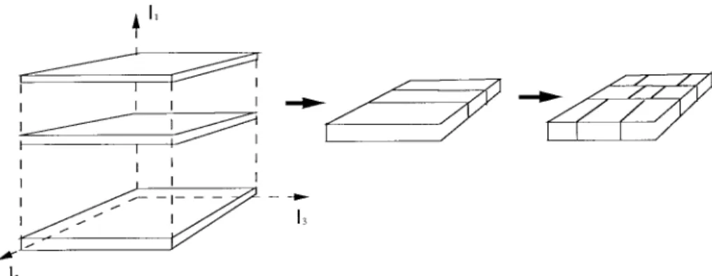
Fig. 1. The partition of color space by the DSQ.
colors in this paper, are extracted by a dependent scalar quantization (DSQ) algorithm and ordered to obtain a sequence of feature vectors. Matching the characteristic colors between a query image and each data-base image is achieved by using a dynamic matching method, which is based on the dynamic programming equation in order to overcome varying viewpoints of the image, occlusion, and varying lighting conditions and to obtain the best match path. A dynamic programming approach has shown great potential in solving difficult problems in optical character recognition (OCR) [20], and especially speech recognition [21]. Combining the DSQ algorithm and the dynamic matching method, a mechanism is proposed for image data-base retrieval. We demonstrate the proposed mechanism with a set of experiments, which compare the performance of existing methods with that of the proposed mechanism.
This paper is organized as follows. The approach to extract-ing the characteristic colors as the color features is presented in Section II. Section III describes how to use the proposed color features to carry out the tasks of image data-base retrieval. Section IV reports the simulation results of the proposed matching method. Conclusions are drawn in Section V.
II. APPROACH TO COLORFEATURE EXTRACTION
In the early perception stages of human beings, similar colors are grouped together to fulfill the tasks of identification. Based on this assumption, we present a scheme in this section to group similar colors of an image and extract the charac-teristic colors as the features for identification. The proposed scheme for extracting the color features is similar to the design of the color palette for an image. It requires quantization of the original full-color image into the limited color image. Among many approaches to the design of the color palette [7], [8], the DSQ approach proposed by Pei and Cheng [9] has been shown to perform well. We employ the DSQ approach to generate a color palette that contains the characteristic colors used as the color features. This approach for the design of the color palette is reviewed below.
A. Dependent Scalar Quantization
As displayed in Fig. 1, the DSQ approach partitions color space of an image in a dependent way in order to fully utilize
the correlations of the color components of an image. The partition used is the 1-D moment-preserving (MP) technique. The advantage of the MP quantizer is that the output can be written in the closed form [10]. When using another fidelity criterion, such as mean square error (MSE) [11], it is usually impossible to obtain a closed-form expression for the quantizer. Also, using this DSQ procedure, the computational cost is rather small.
The DSQ mainly consists of two stages, namely, the bit allocation and recursive binary MP thresholding. Suppose the set of all grid points of the image is denoted by , and its members that belong to may be explicitly written as , where is the row index and is the column index. The color value of is denoted as , where is the associated color component value.
1) Bit Allocation: If the DSQ expects to be unsupervised,
the number of thresholding levels in each color component must be decided a priori. Since the number of thresholding levels can be expressed by powers of two, we choose bits to represent the total thresholding levels. The purpose of the bit allocation is to automatically assign a given quota of bits to each color component of the image, that is, a fixed number of bits has to be divided among the color components, . The bit-allocation method typically assigns more bits to the color components with larger variance and fewer bits to the ones with smaller variance. The reason for this choice is that if the data are very spread out on a particular color component, then presumably the data in that component are more significant than that of other, more densely grouped components.
The significant component should be given more bits in order to reduce the quantization error. If the probability density functions are the same for all the components , except for their variance, an approximate solution to the bit allocation of each component is given by [12]
(1)
where is the variance of the component . After the bit allocation, the number of thresholding levels of each component for has been determined. Then, the recursive binary MP thresholding is used to partition each component.
(a)
(b)
Fig. 2. Recursive binary moment-preserving thresholding.
2) Recursive Binary MP Thresholding: Employing the
bi-nary MP thresholding on a color component , the total pixels are thresholded into two pixel classes, i.e., the below-threshold pixels and the above-below-threshold ones. The problem of binary MP thresholding, as Fig. 2(a) illustrates, is to select a threshold value such that if the component values of all below-threshold pixels are replaced by , and those of all above-threshold pixels are set to , then the first three moments of color component for the image are preserved in the resulting two-level image. Given the color value of each pixel, the th moment of color component is defined as (2a)
where is the total pixel number. The th moment can also be computed from the distribution of values, or histogram, as follows:
(2b)
where is the total distribution levels in the histogram and is the number of pixels with the value in the histogram.
Let and denote the fraction of the below-threshold and above-threshold pixels in the image after the binary MP thresholding. Then the resultant th moments of the two-level image are just
(3)
If we preserve the first three moments of the resultant two-level image equal to those of original image
, we get the following moment-preserving equations:
After some simple computations, can be obtained as
(4) From , the desired threshold is chosen as the -tile of the histogram such that
(5) Now considering partitioning color component into intervals, we use the binary MP thresholding technique re-cursively to obtain the desired thresholding levels instead of directly applying the multilevel thresholding technique as in [10]. The range of the color component , with boundary values zero and , is first partitioned into two
inter-vals and , where represents the
threshold obtained by first binary MP thresholding. Then the interval is partitioned into two subintervals
and , where is the threshold obtained by second binary MP thresholding. Similarly, is partitioned into two subintervals and
by third binary MP thresholding. The above procedures are illustrated in Fig. 2. If we continue the procedure recursively by using the binary MP thresholding times and order the resultant thresholds according to their values, the
output thresholding levels will be
determined, i.e., for .
3) The DSQ Algorithms: Based on the above discussion
of bit allocation and recursive binary MP thresholding, the algorithm to generate the DSQ color palette can be described as follows.
Step 1) Input the image and utilize the bit-allocation pro-cedure to determine the total thresholding levels of each color component.
Step 2) Do the recursive binary MP thresholding on and calculate the associated thresholding levels
.
Step 3) Do the following steps times:
3.1) Perform the recursive binary MP thresholding on of pixels within the rectangular box bounded by and calculate the associated thresholding levels
.
(a)
(b)
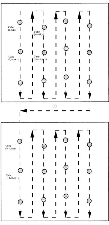
Fig. 3. The ordering of characteristic colors. (a) Layer l. (b) Layer l+ 1.
3.2.1) Calculate the recursive binary MP threshold-ing on of the pixels within the long bar
limited by and
and compute the associated
threshold-ing levels .
Step 4) Assign the centroid of color points inside a cube formed by Steps 2) and 3) as a characteristic color of the color palette.
B. Color Features from the DSQ Approach
After using the DSQ approach, the input colors of the image are grouped into disjoint sets, .
is the predetermined color-palette size. In each set , there
Fig. 4. The images of 27 objects in the first data base.
is a characteristic color chosen. These characteristic colors constitute the color palette. We define
as the set of the color features that represent the original image. The DSQ approach requires
times binary MP thresholding to finish color space partition. It takes approximately multiplication oper-ations for binary MP thresholding. So, the total multiplicoper-ations for the recursive binary MP thresholding will be approximately
.
Furthermore, the partition of color space by the DSQ approach shown in Fig. 1 causes the characteristic colors to be distributed layer by layer in the 3-D space. We arrange these characteristic colors in the 1-D way in order to process them efficiently in the mechanism of image data-base retrieval. As shown in Fig. 3, the characteristic colors are ordered sequentially in the 1-D way, where denotes the index of the associated characteristic color. The value of the index is increasing from the bottom layer to the upper layer. Through this ordering, two neighboring indexes would represent two visually close colors. The image could be represented by a sequence of feature vectors
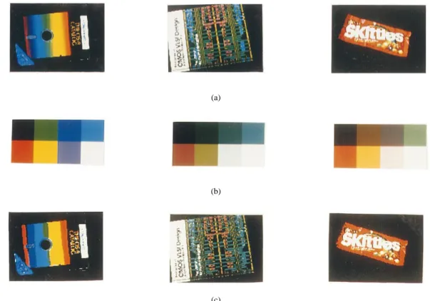
(6) To illustrate the color features extracted by the proposed approach, we have chosen three test images from a data base of 27 images, shown in Fig. 4. The red, green, blue (RGB) images in the data base are 159 119 size coded at eight bits for each color component. For each test image, we utilize the DSQ approach, which allocates three bits to color components, to obtain a color feature set of size eight. Setting in (1), we have acquired for . Thus, binary MP thresholding is used once for each color component in the sequential partition of color space shown in Fig. 1. In Fig. 5, we show test images, the corresponding color feature sets, and the quantized images, which used the characteristic colors in each color feature set to form the associated color palette. It is noticed from Fig. 5(c) that color information inside the quantized images is similar to that of the corresponding test images. That is, the characteristic colors in each color
(a)
(b)
(c)
Fig. 5. Results of the DSQ approach to extract the color feature sets: (a) original images, (b) corresponding color feature sets, and (c) corresponding quantized images by using the characteristic colors to form the color palette.
feature set of Fig. 5(b) can represent color information inside the corresponding image. Therefore, the characteristic colors extracted by our DSQ approach are reliable and able to be used as the color features of the image.
III. MECHANISM OF IMAGEDATA-BASERETRIEVAL
This section describes how to use the sequence of feature vectors, which are the characteristic colors extracted by the DSQ approach, to identify a query image from data-base images. The problem of identification can be described as follows. If is the query image and is one of images in the data base, minimize the distortion between and . The goal thus is to find an image in the data base whose distortion satisfies
for (7)
where is the number of data-base images. Concerning the distortion between two images, we designate it as the distance between two sequences of feature vectors. To calculate this distance, a measure of closeness between two feature vectors has to be found. Since each feature vector is a characteristic color, the measure used in this paper is the color distance. Then we will introduce a dynamic matching method to obtain the distance between two sequences of feature vectors.
A. Color Distance
A color space describing colors close to human perception is crucial in calculating color difference based on color
percep-tual similarity. The RGB color space, which is normally used in the frame grabber of color-processing systems, does not carry direct information about the color. For example, people cannot distinguish between colors by their (R,G,B) triplet. Contrary to the RGB color space, the empirically defined hue, value, saturation (HVC) space, which is a variant of the Munsell color space, expresses colors in terms of triattributes of human color perception. Hafner et al. [16] have found that the HVC color space gives the best performance (using human judgment of the similarity between the query and data-base images) for experiments with a variety of color spaces. Processing color images based on the HVC space, existing processed errors can be evaluated according to how human beings perceive the errors. To calculate color difference in the HVC color space, we adopt Godlove’s formula [13] instead of a Euclidean distance measure. Godlove’s formula defines color difference directly related to the National Bureau of Standards (NBS) unit color difference, which is for the assessment of color difference [17].
There are several ways to mathematically transform between the RGB and HVC color space. The transformation used in this paper involves color space. If a set of RGB color value is given, the transformation of color value from the RGB color space to the HVC color space is as follows [14].
Step 1) RGB color value is first transformed into XYZ color value as
Step 2) A nonlinear process concerned with a human vision model is performed as
where .
Step 3) HVC color value is obtained by the formula
(8)
where and
.
For two colors in the HVC color space, expressed as and , Godlove’s formula of color distance is defined by
(9)
where and
.
B. Dynamic Matching Method
If the conditions of identification of the query image are consistent, the images of the same object captured at different instants will also not differ much in their histograms of color components. The locations of their associated characteristic colors with the same index will thus be close. In this circum-stance, the distance between two sequences of feature vectors can be defined as the sum of color distances between two characteristic colors with the same index . That is
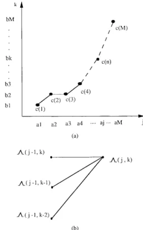
However, due to varying viewpoints of the image, occlusion, and varying lighting conditions, the environment for identify-ing the query image is nonstationary. To find the color distance of two sequences of feature vectors in these situations, we propose a dynamic matching method, depicted in Fig. 6(a), where input sequences and are developed along the horizontal -axis and vertical -axis, respectively. We try to find a path that represents the best match between two input sequences. This best match path is shown as the sequence in Fig. 6(a). After this match path is obtained, we then calculate the color distance of each matched pair of characteristic colors, which are feature vectors from and . Last, the distance between two sequences of feature vectors is defined as the sum of these color distances.
The sequence can be considered to represent the output of matching function from the axis of sequence
(a)
(b)
Fig. 6. (a) Dynamic matching method. (b) Dynamic programming equation of matching function.
onto that of sequence . In Fig. 6(a), we suppose that and are expressed as
where is the index of the characteristic color and is the length of the sequence. and are the characteristic colors with color value . The matching function is denoted as
where . When there is no difference
between and , the matching function coincides with the diagonal line . It deviates further from the diagonal line as the difference grows.
The matching process is normally performed by using a dynamic programming equation [15]. In our case, the equation is given by
(10)
where is the partial sum of distance related to point along the best path from point to point and is the color distance between two matched feature vectors or characteristic colors. Fig. 6(b) illustrates how the partial sum of distance is obtained. In (10), we employ color
(a)
(b)
Fig. 7. (a) The images of 27 query objects. (b) Query images with blurring, 19-dB, and 9-dB degradations from left to right.
TABLE I
COMPARATIVEPERFORMANCE: QUERYIMAGES FORDATABASEI
difference from Godlove’s formula, which is expressed in (9) to calculate .
The summation of color distances by (10) will reach its minimum value when matching function is ob-tained so as to optimally adjust the difference between se-quences and . This minimum distance value is then denoted as the distance between sequences and
(11)
TABLE II
COMPARATIVEPERFORMANCE: QUERYIMAGES OFTABLEIWITHDISTORTION
The computational complexity of the dynamic matching method is mainly due to determining the partial sum of (10) in each point . In (10), it requires three addition calculations, one color distance calculation by Godlove’s formula, and
TABLE III
COMPARATIVEPERFORMANCE: SCALEDQUERYIMAGES FORDATABASEI
Fig. 8. Effects of changing intensity on match success of the proposed method, Swain’s method, Funt’s method, the distance method, and the reference color table method.
one comparison. The total number of processing points is proportional to . If is small—for example, eight in the experiments below, this would not cost too much computational overhead.
IV. EXPERIMENTAL RESULTS
To illustrate the performances of the proposed matching method, we built 27 query images, shown in Fig. 7(a). Com-pared with the first data base shown in Fig. 4, the objects as
(a)
(b)
Fig. 9. The 65 trademark images in the second data base and six query images. (a) 65 trademark images. (b) Six query images:T1; T2; T3; T4; T5, and T6.
TABLE IV
COMPARATIVEPERFORMANCE: QUERYIMAGES FORDATABASEII
shown in Fig. 7(a) are translated, rotated, and occluded. For these query images, we have utilized:
1) Swain’s histogram intersection method [5]; 2) Mehtre’s distance method [6];
3) Mehtre’s reference color table method [6];
4) the proposed dynamic matching method to see if the query objects can be distinguished from the data base of Fig. 4 and to evaluate the sensitivity of the above
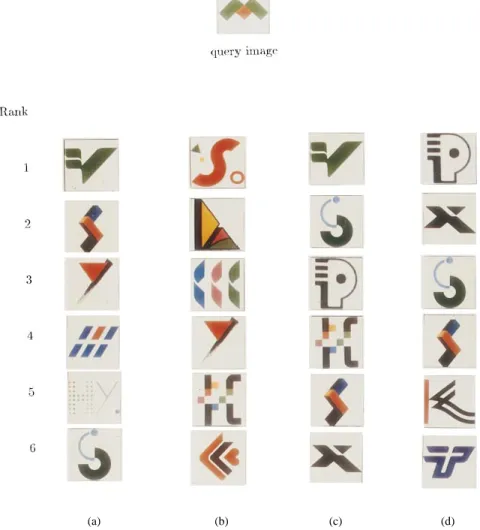
(a) (b) (c) (d)
Fig. 10. Sample query results of different matching methods: (a) Swain’s method, (b) the proposed method, (c) the distance method, and (d) the reference color table method.
matching methods to noise, changes in resolution, and various lighting conditions.
The color space used in the experiments is the RGB space. Concerning the proposed matching method, the length of the sequence of feature vectors chosen is eight. The number of 3-D histogram bins used by Swain’s method is 2048. In the reference color table method, the reference color table contains 27 colors, as suggested by [6]. The matching percentile [5] for each query image is calculated as
matching percentile rank
where is the total number of objects in the data base and
rank is the position of correct match after matched results are
sorted.
Table I shows the matching success of the above testing methods for the query images. As we observe, Swain’s and the proposed methods can correctly identify each query image. To see how noise affects the matching accuracy, we added two sets of Gaussian noise to the query images with the signal-to-noise-ratio (SNR) value defined as
SNR
where , and are the input color component power. , and are the noise color component power. SNR ranges from 19 to 22 dB for the first set of noise and 7 to 12 dB for the second set of noise. For each pixel of every query image, we also blurred the query image by averaging pixel values within an 11 11 window centered at it in order to see how this distortion would affect the matching accuracy. Fig. 7(b) displays one query image with the above added degradations. Table II illustrates the matching success of the testing methods for these noise-added and blurred images. As we observe, the proposed method achieves a better average match percentile than both the distance method and the reference color table method. It missed four query objects in the blurred query images. Swain’s method does not have good matched results for the query images added with the second set of noise as compared with the proposed method. In these empirical results, our current implementation of the DSQ algorithm and the dynamic matching method takes less than 2 s of CPU time to process a query image with size 159 119 on a SunSPARC Station 10. Of this total time, about 1 s is needed for the DSQ approach; about 1/3 of a second is needed for matching the query image with one image in the data base.
(a)
(b)
Fig. 11. (a) The 61 images in the third data base. (b) Query results by the proposed method.
The effect of reducing the resolution of the query images is investigated and shown in the Table III. As we see, the proposed method performs the best among the testing methods, especially for the resolution 9 7. To simulate the changing lighting condition, we have multiplied the image pixel values by a constant factor ranging from 0.5 to 1.5 for each query image. The resultant pixel values were constrained to be no greater than 255. The transformed images were then matched to the data base of Fig. 4. The results are displayed in Fig. 8. In this simulation, we have also included Funt’s method [18], which is specifically designed to be invariant to lighting. Except for our method and Funt’s method, the matching accuracy is degraded significantly when the factor
values approach 1.5 and 0.5. As we know, the effect of multiplying each pixel with a factor value would cause the histogram of color components to be changed notably. For the histogram-matching methods, like Swain’s method and the color reference table method, this multiplication effect thus lowers the matching accuracy. Since Funt’s method uses the ratios of color RGB triples from neighboring locations, its results are constant for this simulation. As can be verified, Funt’s method has the best performance for a factor value of 1.5. On the other hand, since the order of the sequence of feature vectors does not change too much by these values of factor, our method generally has good performance as compared with the other testing methods. However, with a
multiplication factor larger than 1.5, it is expected that the matching accuracy of our method will degrade gradually.
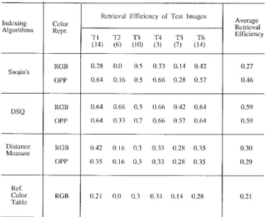
In addition, we constructed a second data base of 65 trademark images to test another image data-base retrieval scenario. Given a query image, we want to obtain a list of images from the trademark data base that most resemble colors in the query image. We captured six query images, designated from T1 to T6, and manually listed the resembling images found in the data base for each query image. Each data-base and query image with size 128 128 consists of 8-bit “red,” “green,” and “blue” color components. The data-base and query images are displayed in Fig. 9. Let be the number of manually listed images for each query image. We applied the above testing methods to each query image. A list of images with size for each query image is then created to check how many images are correctly matched. If is the number of such matched images, the retrieval efficiency can be defined as follows:
In Table IV, we show the retrieval efficiency of each query image for two color spaces, the RGB and opponent color axes [5], with shown below the notion of each query image. As we observe, the proposed method has better average retrieval efficiency than the other testing methods for this trademark retrieval scenario. The performance of the RGB and that of the opponent color axes is similar for the proposed method. However, for Swain’s method, opponent axes have better results. The retrieval results of the second query image for the RGB space is also illustrated in Fig. 10.
Finally, we have applied the proposed method to a data base of more natural images with a wider range of colors in order to give more insight into its performance. The data base shown in Fig. 11(a) is populated by 61 color images, which have 8-bit “red,” “green,” and “blue” color components. Each time, we picked a color image from the data base as the query sample in order to retrieve the top four images that most resembled in colors. Fig. 11(b) displays three examples of image retrieval. Although the first candidate may not subjectively be the best match, it can be observed that all the retrieved images contain color content quite similar to the query sample. To accurately rank retrieved images, we understand that other features like shape, texture, and color histogram can be adopted. This approach is still open for further study.
V. CONCLUSION
This paper presents an approach of color feature extraction for image indexing. This approach, called DSQ, is similar to the design of a color palette for an image. The DSQ approach first extracts the characteristic colors, which contain color information of the image, by sequentially quantizing color components. The chosen characteristic colors are then ordered to obtain a sequence of feature vectors. Using this sequence of feature vectors, a matching method, called the dynamic matching method, is proposed to carry out the task of image data-base retrieval. The proposed method is mainly based
on the dynamic programming equations to obtain the best match path between two input sequences of feature vectors. The color distance used to obtain the best match path is Godlove’s formula for the HVC color space. The experimental results show that the characteristic colors are reliable color features for image indexing. The proposed matching method has acceptable accuracy of image retrieval as compared with existing color indexing methods mentioned in Section IV. In addition, we have analyzed the computational complexity for both the DSQ approach and the dynamic matching method. Our results show that the proposed method is feasible for implementation.
ACKNOWLEDGMENT
The authors would like to thank the anonymous reviewers, who made many useful comments. Their help is gratefully appreciated.
REFERENCES
[1] T. L. Kunii, Visual Database System. Amsterdam, The Netherlands: Elsevier, 1989.
[2] E. Knuth and L. M. Wegner, Visual Database System II. Amsterdam, The Netherlands: Elsevier, 1992.
[3] R. M. Haralick and L. G. Shapiro, Computer and Robot Vision. Reading, MA: Addison-Wesley, 1993.
[4] G. Healey, “Using color for geometry insensitive segmentations,” J. Opt.
Soc. Amer. A, vol. 6, pp. 920–937, June 1989.
[5] M. J. Swain and D. H. Ballard, “Color index,” Int. J. Comput. Vision, vol. 7, no. 1, pp. 11–32, July 1991.
[6] B. M. Mehtre, M. S. Kankanhalli, A. D. Narasimhalu, and G. C. Man, “Color matching for image retrieval,” Pattern Recognit. Lett., vol. 16, pp. 325–331, Mar. 1995.
[7] P. Heckbert, “Color image quantization for frame buffer display,”
Comput. Graph., vol. 16, no. 3, pp. 297–307, July 1982.
[8] M. T. Orchard and C. A. Bouman, “Color quantization of images,” IEEE
Trans. Signal Processing, vol. 39, pp. 2677–2690, Dec. 1991.
[9] S. C. Pei and C. M. Cheng, “Dependent scalar quantization of color images,” IEEE Trans. Circuits Syst. Video Technol., vol. 5, pp. 124–139, Apr. 1995.
[10] W. Tsai, “Moment preserving thresholding: A new approach,” Comput.
Vision, Graph., Image Processing, vol. 29, pp. 377–393, 1985.
[11] S. P. Lloyd, “Least square quantization in PCM,” IEEE Trans. Inform.
Theory, vol. IT-28, pp. 129–137, Mar. 1982.
[12] A. Segall, “Bit allocation and encoding for vector sources,” IEEE Trans.
Inform. Theory, vol. IT-22, pp. 162–169, Mar. 1976.
[13] I. H. Godlove, “Improved color-difference formula, with application to the perceptibility and acceptability of fadings,” J. Opt. Soc. Amer., vol. 41, pp. 760–772, 1951.
[14] M. Miyahara and Y. Yoshida, “Mathematical transform of (R, G, B) color data to Munsell (H, V, C) color data,” in Proc. SPIE Visual
Communication and Image Processing, 1988, vol. 1001, pp. 650–657.
[15] R. Bellman and S. Dreyfus, Applied Dynamic Programming. Prince-ton, NJ: Princeton Univ. Press, 1962.
[16] J. Hafner, H. S. Sawhney, W. Equitz, M. Flickner, and W. Niblack, “Ef-ficient color histogram indexing for quadratic form distance functions,”
IEEE Trans. Pattern Anal. Machine Intell., vol. 16, pp. 729–736, July
1995.
[17] D. B. Judd and G. Wyszeki, Color in Business, Science, and Industry. New York: Wiley, 1963.
[18] B. V. Funt and G. D. Finlayson, “Color constant color indexing,” IEEE
Trans. Pattern Anal. Machine Intell., vol. 17, pp. 522–529, May 1995.
[19] D. Slater and G. Healey, “The illumination-invariant recognition of 3D objects using local color invariants,” IEEE Trans. Pattern Anal. Machine
Intell., vol. 18, pp. 206–210, Feb. 1996.
[20] K. S. Fu, Y. T. Chien, and G. P. Cardillo, “A dynamic programming approach to sequential pattern recognition,” IEEE Trans. Pattern Anal.
Machine Intell., vol. PAMI-8, pp. 313–326, May 1986.
[21] H. Sakoe and S. Chiba, “Dynamic programming algorithm optimization for spoken word recognition,” IEEE Trans. Acoust., Speech, Signal
Soo-Chang Pei (S’71–M’86–SM’89) was born in
Soo-Auo, Taiwan, R.O.C., in 1949. He received the B.S.E.E. degree from National Taiwan University, Taipei, in 1970 and the M.S.E.E. and Ph.D. degrees from the University of California, Santa Barbara, in 1972 and 1975, respectively.
He was an Engineering Officer in the Chinese Navy Shipyard from 1970 to 1971. From 1971 to 1975, he was a Research Assistant at the University of California, Santa Barbara. He was a Professor and Chairman of the Electrical Engineering Department of Tatung Institute of Technology from 1981 to 1983. Presently, he is a Professor in the Electrical Engineering Department of National Taiwan University. His research interests include digital signal processing, image processing, optical information processing, and laser holography.
Dr. Pei is member of Eta Kappa Nu and the Optical Society of America.
Ching-Min Cheng was born in Taipei, Taiwan,
R.O.C., in 1959. He received the B.S.E.E. de-gree from the National College of Marine Science and Technology, Keelung, Taiwan, in 1982, the M.S.E.E. degree from the University of California, San Diego, in 1986, and the Ph.D. degree in elec-trical engineering from National Taiwan University, Taipei, in 1996.
From 1983 to 1984, he was an Engineering Of-ficer in the Chinese Airforce Anti-Aircraft Corps. From 1986 to 1989, he was a Patent Examiner with the National Bureau of Standards. Since September 1989, he has been with the Telecommunication Laboratories, Ministry of Communications, Taipei, Taiwan, as a Research Engineer. His research interests include digital signal processing, video compression, and multimedia communication.