A multiparameter analysis of domino tiling with an application to concurrent systems

Theoretical Computer Science 98 (1992) 263-287 Elsevier

263

A multiparameter

analysis of

domino tiling with an application

to concurrent systems

Hsu-Chun

Yen

Deparlment of Electrical Engineering, National Taiwan University, Taipei, Taiwan, Republic of China

Communicated by A. Salomaa Received December 1989 Revised July 1990

Abstract

Yen, H.-C., A multiparameter analysis of domino tiling with an application to concurrent systems, Theoretical Computer Science 98 (1992) 263-287.

The complexities of two domino problems, namely the (n, k) domain problem and the (n, k) 2-person domino game problem, will be investigated with respect to parameters n and k simultaneously. The former concerns itself with tiling a rectangle of width k in the Cartesian plane using a given set of n domino types. The latter involves two players taking turns to tile a rectangle of width k using a given set of n domino types in an antagonistic fashion. (We are interested in determining whether there is a winning strategy for the first player.) It turns out that the (n, k) domino problem has upper and lower bounds of ti(k * log n) and Q(((k - 6)/2) * log n) nondeterministic space, respectively. For the (n, k) 2-person domino game problem, we are able to show upper and lower bounds of O(n”‘) and R(n’k-5)“6-E) deterministic time, respectively, for some constant c, any e@O and k> 17. Using the result concerning the 2-person domino game problem, we then establish a lower bound of Q(nc’-7”‘6-E) deterministic time, any &>O and k>21, for the lockout problem for systems of k communicating processes in which the size of each process is bounded by n. This, together with an O(d”) deterministic time upper bound (which will also be shown in this paper), fully explains the role played by each of the two parameters (n and k) in the overall complexity of the problem. (It indicates that the upper bound is optimal with respect to parameters n and k.)

1. Introduction

Domino problems, first introduced by Wang [19] more than two decades ago, have been gaining more and more popularity over the past few years. The merit of domino tilings comes from the fact that dominoes are structurally simple and conceptually easy to visualize. Furthermore, they represent a unified model for which many 0304-3975/92/$05.00 0 1992-Elsevier Science Publishers B.V. All rights reserved

important complexity classes can be defined in a natural way. As a result, they provide proofs which are easy to present and understand, compared to those involving brute-force reductions from Turing machines.

A domino is a 1 x 1 square tile with colored edges. Assuming that we have an unlimited supply of copies of each domino type, the domino problem is that of determining, given a set T of domino types, whether a grid region (bounded or unbounded) in the Cartesian plane can be covered using only dominoes from T such that adjacent dominoes have matching colors along their common boundaries. In the literature, a number of variants of domino problems have been shown to be undecid- able. The most natural and general unbounded domino problem, i.e., the problem of determining whether the plane can be tiled using the dominoes from a given set of domino types, was proved undecidable by Berger in [2]. By imposing an additional constraint that certain domino types (or colors) occur infinitely often, Hare1 [6, 71 subsequently introduced the so-called unbounded recurring domino problems as a vehicle for showing highly undecidable lower bounds such as Z : (the first level of the analytical hierarchy). See [6, 73 for more about unbounded recurring domino prob- lems and their applications to logic. Bounded domino problems, proposed by Lewis [12], involve tiling bounded regions in the Cartesian plane. In the literature, various bounded domino problems have been shown to be complete for a wide spectrum of complexity classes, including NP, PSPACE, EXPTIME, 2EXPTIME and, more recently, the entire polynomial-time hierarchy. They have also been shown to be very useful, as a reduction tool, for proving lower bound results. (See e.g. [3, 4, 5, 13, 16, 181.)

The goal of this paper is to incorporate the idea of multiparameter analysis into domino problems, thus providing a tool for analyzing problems for which multiple parameters are involved. By multiparameter analysis, we mean the technique of studying the complexity of a problem in terms of two or more natural parameters simultaneously and of revealing the role played by each parameter in the overall complexity, as opposed to examining the problem when one (or more) of the para- meters is fixed.

To motivate our work, we consider an example concerning concurrent systems. (The problem will be studied in greater detail later.) Suppose we are given a system of k concurrent processes P = ( PI, . , Pk). Let (PiI be the size of process Pi (when some standard binary encoding scheme is used). So 1 P I< k * n, where n is max { 1 PI 1, . . . , ) Pk ) } (i.e., the maximal size of all processes). Consider the lockout problem defined by Ladner in [l 11. Roughly speaking, the lockout problem is that of determining, given a system of processes, a process Pi and a set of states Q (of Pi), whether Pi will be locked out of Q by the rest of the system. More precisely, can the rest of the system “conspire” in such a way that Pi will be denied from entering Q forever? The lockout problem was shown to be EXPTIME-complete by Ladner in [ 111. There the complexity bound was measured in terms of the size of the system, i.e., (PI. Since EXPTIME is beyond the scope of any tractable computation, it is therefore of practical interest to know whether the problem will become tractable when a certain constraint is imposed. By

Multiparameter analysis of domino tiling 265 carefully examining the proof in [ 111, it is not hard to see that the problem is solvable in O(nc*k) deterministic time, for some constant c, meaning that if the number of communicating processes (i.e., k) is a fixed known constant, then the problem can be solved in polynomial time. However, this result does not preclude the existence of an O(nd + 2k) deterministic time algorithm (for some constant d). We shall provide, in this paper, a simultaneous lower bound over parameters n and k for the lockout problem by exhibiting a lower bound of fi(nck-7”‘6-E ) deterministic time, for any k > 21 and E>O. As a consequence, the O(nc*k) upper bound is optimal with respect to both n and k.

So far, not many problems have appeared in the literature which are examined in terms of two or more parameters simultaneously. Problems requiring Q(n”) determin- istic time were previously shown in [l]; while problems requiring Q( k * log n) non- deterministic space were considered in [9]. In [14], the boundedness problem for vector addition systems with states was shown to have upper and lower bounds of 0(2 2 * k*‘og k( 1+ log n)) and Q(2d*k( I + log n)) nondeterministic space, respectively, where k is the dimension of the vector addition system with states, 1 is the maximum size of any integer mentioned, n is the number of states and c and d are constants. Rosier and Yen [15] dealt with the multiparameter complexity of the fair nontermina- tion problem for systems of probabilistic concurrent finite-state programs with respect to various fairness constraints. In [20], the complexity of the nontermination problem for systems of communicating processes was studied in terms of two natural para- meters, namely, the number of processes and the size of the maximum process, with respect to different scheduling methods.

In this paper, we begin with a multiparameter analysis of a domino problem, known as the rectangle tiling problem. It is the problem of determining, given a set T of domino types and a k (in unary), whether any rectangle of width k can be tiled using T. This problem was first studied in [12] and was shown to be PSPACE-complete, provided k is part of the input. We will provide a refinement of the PSPACE result by showing that the rectangle tiling problem has lower and upper bounds of Q((( k - 6)/2) * log n) and 0 (k * log n) nondeterministic space, respectively, where n is the number of types of dominoes in T. As a consequence, the problem is PSPACE- complete in k and is solvable in NLOGSPACE, provided k is a fixed constant.

Another problem to which we shall apply the multiparameter analysis technique is the 2-person rectangle tiling game, introduced by Chlebus in [3]. In this game, two players, say CONSTRUCTOR and SABOTEUR, take turns to tile a rectangle. The 2-person rectangle tiling game problem is to determine whether CONSTRUCTOR has a winning strategy regardless of how SABOTEUR counter-moves. It turns out that this problem is EXPTIME-complete [3]. In this paper, we demonstrate lower and upper bounds of Cl(n(k-5)‘16-E) (f or any k>

[l 11) requires Cl(n(k-7)‘16-e) deterministic time, for any k > 21 and E > 0, for systems of k communicating processes in which the size of each process is bounded by n (when a standard binary encoding

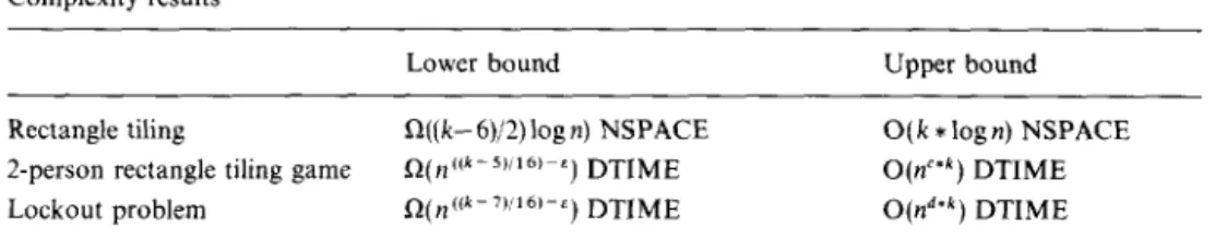
Table 1 Complexity results

Lower bound Upper bound

Rectangle tiling

2-person rectangle tiling game Lockout problem Q((k- 6)/2) log n) NSPACE qncck-5)/16)~c) DTIME ,(,((k-7)!16)-&) DTIME 0( k * log n) NSPACE O(n’*‘) DTIME O(n”‘k) DTIME

scheme is used). This clearly illustrates the role played by the degree of concurrency

(i.e. k) in the complexity of the lockout problem. As a result, if the number of processes

is a fixed constant, the problem can be solved in polynomial time. However, the order

of the polynomial grows linearly as the number of processes increases. A summary of

our results is presented in Table 1.

The key contributions of this paper include the following:

(1) For the first time, we show some domino problems suitable for characterizing

complexity classes involving multiple parameters.

(2) We provide refinements over some previously known results, including com-

plexities of the rectangle tiling problem (of [IZ]), the 2-person rectangle tiling game (of

[3]), and the lockout problem for systems of communicating sequential processes

(of

Clll).

(3) Our application to concurrent systems, to some degree, seems to open a new

area of application for domino problems. That is, our work provides concrete

evidence to suggest that domino problems might be useful for proving lower bounds

for problems concerning concurrent systems.

The remainder of this paper is organized as follows. In Sections 2 and 3, we review

some basic definitions, notations and results of complexity theory which will be used

in subsequent sections. Section 4 concerns itself with incorporating multiparameter

analysis techniques into two rectangle domino tiling problems. In Section 5, the

complexity

of the lockout

problem for systems of communicating

processes

will be investigated (using results from Section 4) with respect to two natural para-

meters.

2.

In this section, we review some basic notations and results of complexity theory that

we shall use later in this paper. Unless otherwise stated, we use multitape

machines

(TMs) as the model of computation.

We denote by DTIME(f(n))

Multiparameter analysis of domino tiling 261

TMs using at most f(n) time, where IZ is the length of the input. Similarly,

DSPACE(g(n)) (NSPACE(g(n)) denotes the class of languages accepted by determin-

istic (nondeterministic) TMs using at most g(n) space in the course of the computation.

Let

DLOGSPACE = DSPACE(log n)

NLOGSPACE = NSPACE(log n)

PTIME = UkE,~~l~~(nk)

NP= UkE,~~l~~(nk)

PSPACE= U,,,DSPACE(~~)

EXPTIME = UkENDTIME(2”‘)

It is well known that DLOGSPACE c NLOGSPACE c PTIME E NP E PSPACE s

EXPTIME. Given two languages

and

is said to be

reducible (polynomial-time many-one reducible)

to

denoted

by

(L,-jj: L,)

iff there exists a TM transducer

operating in DLOGSPACE (PTIME)

such that for all x,

iff

Throughout

the rest of this paper, we shall

use logspace many-one

reductions, unless stated otherwise. (Hence, we abbre-

viate SE, by 5.) Let V be a complexity class. A language

is said to be

for %’

iff for every LIE%?,

is said to be

for %? iff

is in %Y

and

is hard

for %Y. For complete problems concerning

complexity

classes DLOGSPACE,

NLOGSPACE,

PTIME, NP, PSPACE, EXPTIME, the reader is referred to [S].

Let C={O,l}. A mapping g:C*+C

* is said to be

in S(n) space

time) iff there exists a deterministic TM M such that, given an input XEC*,

will

output g(x) using at most S( Ix I) space

time). Now, consider two problems

L

and

over C *,

is said to be (S(n), Q(n)),,,,,- reducible

(n)),,,,-reducible) to

L’ iff there exists a mapping g computable in S(n) space

time) such that

(1)

iff

and

(2) vx~C*,

Is(x)I~Q(l~l).

Let %? be a class of problems over C.

is said to be

with respect to

6%

QLpace-

reducibility

Q),i,,-reducibility) if for every L’ in %‘,

there exists a constant

c such that L’ is (S(n), c * Q(n)),,,,,- reducible ((T(n),

Q(n)),i,,-reducible) to

[9].)

The following results were given in [9].

Lemma 2.1. If

a

M with tape symbols (0, 1,

#}

log

symbols (0,

l}.

Lemma 2.2. Let L ( EZ*) be W-hard with respect to (S, Q),,,,,reducibility. Zf L is

solvable in S’(n) nondeterministic space, then for any problem L’ in %?, there are constants cl and c2 such that L’ is solvable in S”(n) + c2

log

Lemma 2.3. Given two languages L, and L2, suppose L1 is (T(n), Z(n)),i,,-reducible to

L2. If L2 can be solved in T2(n) deterministic time and T(n)@ T2(Z(n)), then L1 can be solved in T,(Z(n)) deterministic time.

3. Domino problems

A domino is a 1 x 1 unit square tile whose edges are colored and whose orientation is fixed. We denote by (left-color, right-color, bottom-color, top-color) a domino type, representing dominoes whose left, right, bottom, and top edges are colored left-color, right-color, bottom-color and top-color, respectively. Pictorially, Fig. 1 shows a domino of type (a, b, c, d). Given a domino type d, we use left(d), right(d), top(d) and

bottom(d) to denote the left, right, top and bottom colors of d, respectively. For a set of

domino types T, we define Color(T) to be {left(d), right(d), top(d), bottom(d) 1 de T}, i.e., the set of colors appearing in T. Assuming that we have an infinite supply of copies of each domino type, the domino problem is that of determining whether a (finite or infinite) grid region in the Cartesian plane can be tiled using dominoes from T such that some specific constraints are met. Let G(width, height) represent the region

((x,y)IO<xbwidth, O<y<height}, where width and height are in Nu{co). (For example, G(co, co) represents the first quadrant.) A domino system is a tuple

(T, G(width, height),f), where

(1) T is a set of domino types, (2) G(width, height) is a region, and

(3) f: { 1,2, . . , width} x { 1,2, . . . , height} + T is the tiling function.

(For convenience, we use fi,j to denote f(i,j) throughout the remainder of this paper.) h,j can be thought of as the domino (in the tiling defined by f) whose upper right-hand corner is located at coordinates (i,j). A domino system

(T, G(width, height),f) is said to have a solution iff

(1) Vi, 1 gi<width, bottom(fi,l)=“White”,

(2) Vi, 1 <id width, top(~,heisht)=“White” if height < co,

(3) Vj, 1 <j<height, lef(f~,j)=“White”,

(4) Vj, 1 <j<height, right(f,,,,,j)=“White” if width< CO,

(5) V&j, l<i<width, l<j<height, lefi(fi,j)=right(f,_,,j), and V&j, l<i<width, 1 <j< height, bottom(fi,j)= tOp(f,,j- 1).

In words, (l)-(4) ensure that external edges are colored “White”. (5) ensures that adjacent edges of dominoes have matching colors. The domino problem is that of

d

•;3

c

Multiparameter analysis of domino tiling 269

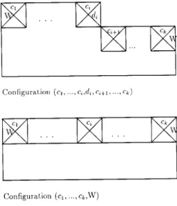
Configurat>ion (c,, . . . . c,,d,, c,+,r . . . . Q)

Configurat,ion (cl, .._, ck,LV)

Fig. 2. Domino configurations.

determining, given T and G, whether there exists an f such that the domino system

(T, G, f) has a solution.

Given a (finite or infinite) region G of width k, we define a conjiguration with respect to G to be a (k+l)-tuple ([C1,,didi,ci+l)..., ck), describing a partial tiling as shown in Fig. 2. (-1, W) denotes a configuration in which the current row is completely tiled.) Given two configurations a1 and az, we write al 5 a2 iff placing d in its appropriate position in a, will result in configuration u2.

A 2-person domino game, introduced by Chlebus [3], consists of two players, CONSTRUCTOR and SABOTEUR, taking turns to tile a finite region using a given set of domino types. CONSRUCTOR plays the first move by placing a domino in the lower left-hand corner. SABOTEUR then selects a domino for the second column and first row. Then CONSTRUCTOR selects a domino for the third column and first row, and so on. This sort of alternation continues until either the region is completely tiled or neither player is able to move. CONSTRUCTOR wins if the tiling is successful; otherwise, SABOTEUR wins. (At any time, if no legal move is available, then SABOTEUR wins.) We require that SABOTEUR must always select a tile that does not violate the tiling property if such tiles exist. A 2-person domino game is said to have a winning strategy for CONSTRUCTOR 8 CONSTRUCTOR can al- ways manage to win regardless of SABOTEUR’s counter-moves. (The goal of CONSTRUCTOR is to finish the tiling, while SABOTEUR will try all he can to prevent this from happening.) In [3], three versions of 2-person domino game problems, namely, square tiling game, rectangle tiling game and high tiling game, have been shown to be complete for PSPACE, EXPTIME, and 2EXPTIME, respectively. Recently, Grade1 [S] has used domino games to characterize the entire polynomial- time hierarchy.

In Section 4, we shall investigate the complexity of each of the following two problems as a function of two natural parameters II and k:

(1) The (n, k) domino problem: Given a set T of n domino types and a keN, does there exist an mEN such that the region G(k,m) can be tiled using T?

(2) The (n, k) 2-person domino game problem: Given a set T of n domino types and

a kEN, does there exist an mEN such that CONSTRUCTOR has a winning strategy in tiling region G(k,m)?

4. Complexity results

We first deal with the (n, k) domino problem. As mentioned earlier, the main concern here is to investigate the overall complexity of the problem as a function of parameters n and k. As defined in [9], we let NLI, be the class of languages accepted by nondeterministic Turing machines in k * log n space using binary tape symbols (i.e., its tape alphabet is (0, 1)).

Theorem 4.1. NLI, is reducible to the (O(n’ log n), k) domino problem with respect to

((2 + E) * log n, n* log* n),,,,,reducibility.

Proof. Let M be an arbitrary k * log n space bound nondeterministic Turing machine whose tape alphabet is (0, l}. Consider an arbitrary input string x. (Let n = 1x1.) In what follows, we show how to construct a set of domino types T, consisting of

O(n* log n) domino types, to simulate the computation of M on x in such a way that

M accepts x iff G(k,m) can be tiled by T, for some meN. We assume that each

transition of M is of the form

(

symbol to b’ and move its input and work tape heads in directions d, and

d2 (dl,d2E(1, -l}), respectively.

The basic idea behind our proof is similar to that of using dominoes to simulate the computation of a general Turing machine. (See, for example, [13].) Basically, each row is used to encode, using appropriate colors, the contents of the k *log n work tape cells, the current state as well as the current input and work tape head positions. Furthermore, the execution of a transition (of M on x) corresponds to the action of tiling two adjacent rows in the upward direction. (The unfamiliar reader is referred to [13] for more details.) The key difference here is that the width of our region is limited to k. As a result, more involved simulation of the TM tape is needed. We divide the

k * log n work tape cells into k blocks of length log n bits each. By doing so, we will

then be able to simulate each block (of length log n) by a single domino. (Overall, only polynomial (in n) number of dominoes are required.)

Multiparameter analysis of domino tiling 271

We are now in a position to construct T. The top edge color of each domino belongs to the following:

(1) “W” (“white”),

(2) i, 06 i<n (representing the tape contents of a block), or (3) q i

( Pl P2 1 ’

where 0 < i < n, qEQ, 1 d p1 < n and 1 d p2 <log n. In words, q, i, p1 and p2 represent the current state, the tape contents of a block, the current input head position, and the displacement of the current tape head position within the scanned block, respectively. (For convenience, “(” and “)” are omitted in all figures.)

Assuming that initially M is in state qO, the input head (work tape head) is scanning the first cell of the input tape (work tape), and the work tape cells are all 0, T consists of the dominoes shown in Figs. 3-8. More precisely, they are:

(1) The dominoes described in Fig. 3 are used to force the bottom row of dominoes to encode the initial configuration of M on x.

(2) For each i, O<i<n, T contains the domino type depicted in Fig. 4.

(3) Whenever (q,a,b)-+(q’, b’,dI,d2) appears in M (assuming that q is not an accepting state) and

x( pI)=a (the pith symbol of x is a),

i(p2)= b (the p,th position of the work tape in the current block contains i’(p,)=b’, i’(j)=i(j), Vj#p2,

P;=PI+dI, P;=P2+d2,

(a) if 1 <p2 + d2 <log n (i.e., the new work tape head remains in the same then T contains the domino shown in Fig. 5.

block), (b) if p2 +d, =0 (i.e., the work tape head moves to the previous block), then

T contains the dominoes shown in Fig. 6.

(c) if p2 +d, = log n + 1 (i.e., the work tape head moves to the next block), then

T contains the dominoes shown in Fig. 7.

pig

pJ

Da

w

w

Fig. 5.

Fig. 6.

Fig. 7.

q

is

vo < j <

Fig. 8.

(4) The dominoes shown in Fig. 8 are used for completing the roof (top row) when

M reaches an accepting state.

As stated earlier, the claim of the construction is that the color of the (top) boundary in each row corresponds to a reachable configuration of M on x. In addition, two adjacent rows correspond to the execution of a transition of M. These facts can easily be verified from the above construction. If, at some point, M enters an accepting state, one can then complete the tiling by placing a row on top using appropriate dominoes (those belonging to the last category).

Now we calculate the size of T(i.e., the number of types in T). It is fairly easy to see, from the above construction, that this quantity is bounded by 0(n2 logn). Hence,

Multiparameter analysis of domino tiling 213

T can be written in O(n’ log2 n) bits. Now we describe the Turing machine transducer

D that, when given x, produces T. The work tape of D is of the following form for each of the above domino categories:

(1) # i #, i is of constant length. (2) # i #, i is of length log n bits.

(3) (4) # i # j # I #, i is of length log n (for representing the contents of a block), j is of length log n (for representing the input head position) and 1 is of length log log n (for representing the work tape head position).

Overall, D requires no more than 2 + log II + log log n bits plus some # ‘s. According to Lemma 2.1, the construction can be carried out in deterministic space ((2 + E) * log n), for any E > 0. 0

Corollary 4.2. For k > 6, the (n, k) domino problem requires sZ( (( k - 6)/2) * log n) non-

deterministic space.

Proof. Assume that the problem can be solved in ((k - 6)/2 -E) * log n nondeterminis- tic space, for some k > 6 and E > 0. According to Theorem 4.1, the problem is NL,-hard with respect to ((2 + ai) * log n, n2 log2 n)space reducibility, for any .sl > 0. From Lemma 2.2, we have that any language in NLI, can be solved in S”(n) + c2 log S’(n) nondeter- ministic space, where S”(n)=(((k-6)/2-e)*log(cIn210g2 n))+2 *log(cIn210g2n)+

(2 + Ed) * log n. This amount is in (k - 2.5 + s1 + s2) * log n space, for any s2 >O. Since

s1 and s2 are arbitrary, we can pick s1 and s2 such that the amount is in (k - e3) * log n, for some sj >O, which is a contradiction of the result of [17]. (In [17], it was shown that for any E>O, NL, is a proper subset of NL,.,.) 0

Now the upper bound.

Theorem 4.3. The (n, k) domino problem can be solved in O(k * log n) nondeterministic

space.

Proof. First note that it takes k *logn bits to record a domino configuration. As a result, one can employ an 0( k * log n) space nondeterministic search procedure to test whether the configuration (m,W) is reachable. 0

In what follows, we consider the case when the parameter k is part of the input and is represented in unary. Recall that each domino is represented by a four tuple. Hence, the size of an (n, k) domino problem (when the standard binary encoding scheme is used) is k + 4 * n * log n. (log n bits are sufficient to uniquely describe a color; as a result, the set of n dominoes can be represented in 4 *n* logn bits. Also notice that k is assumed to be in unary.) Let h = k + 4 * n * log n be the overall size of an instance of the

(n, k) domino problem. According to Theorem 4.3, the (n, k) domino problem can be

solved in O(k * log n) nondeterministic space, which is in O(h * log h) nondeterministic space since k, n < h. Hence, the problem is in PSPACE. To show the lower bound,

consider the language accepted by an arbitrary nondeterministic Turing machine using p(n) space, where n is the size of the input and p(n) is a polynomial in n. Clearly, the language is in NLp(nJilogn. According to Theorem 4.1, any language in NLp(nj,logn can be reduced to the (O(n’ log n), p(n)/log n) domino problem. This implies that the domino problem is PSPACE-hard if the parameter k (in this case, k = p(n)/log n) is part of the input. (Note that k = p(n)/log n is bounded by a polynomial.) (From the statement of Corollary 4.2, it can also be observed that the amount of space required by the (n, k) domino problem is polynomial in k.)

Thus, we have the following corollary.

Corollary 4.4. Zf k is not fixed (i.e. k is part of the input) and is written in unary, then the (n, k) domino problem is PSPACE-complete.

We now turn our attention to the (n, k) 2-person domino game problem. We are again concerned with a multiparameter analysis of the problem. We shall prove that the (n, k) 2-person domino game problem has lower and upper bounds of Q(n (k-5)‘16-E) and O(nclk) deterministic time, respectively, for any E >O and some constant c. Before proving this, we require the following definitions.

A two-person pebble game G is a 4-tuple (N, R, S, T), where l N is a finite set of nodes,

l R(sNxNxN)isthesetofrules,

l S (EN) is the set of initial nodes, l T (EN) is the terminal node.

G is said to be an (n, k)-pebble game iff 1 N I = n and 1 SI = k. Initially, pebbles are placed

on initial nodes, i.e., all nodes in S. The playing (pebble-moving) rule is that, whenever (x, y, Z)E R and nodes x and y, but not z, contain pebbles, a pebble can be moved from x to z. Two players, say A and B, take turns moving the pebbles. Each player can make at most one move during his turn. A winning position (or win) for a player is when he either moves a pebble to T, or he forces his opponent to be unable to move. At such a time the game is over. The pebble game problem, given a pebble game, is to determine whether the first player has a winning strategy, i.e., whether the first player can always manage to win regardless of his opponent’s moves. As one can easily see, the pebble game problem possesses characteristics similar to that of the computation of an alternating Turing machine (ATM). More precisely, the moves of the first player, when trying to obtain a winning position (regardless of how his opponent moves), corres- pond to the existential branches in an ATM; while the moves of the second player, when trying to prevent the first player from winning, correspond to the universal branches in an ATM. Because of this alternating behavior, the pebble game problem requires exponential execution time. In fact, the following result concerning the complexity of pebble game problem was shown in Cl]: The (n, k)-pebble game problem

requires Q(n(k-‘)14-E ) deterministic time for any E>O and k> 5 on multitape Turing machines.

Multiparameter analysis of domino tiling 21s To derive the complexity for the (n, k) 2-person domino game problem, we begin by proving the following theorem.

Theorem 4.5. The (n, k) 2-person pebble game problem is (O(n4 log’ n), n4 log n)time-

reducible to

l the (O(n4), k + 3) 2-person domino game problem if k is odd, l the (O(n4), k+4) 2-person domino game problem if k is even.

Proof. Let G = (N, R, S, T) be an (n, k)-pebble game between players A and B. We first consider the case when k is odd. In what follows, we show how to construct an

(O(n4), k + 3) 2-person domino game problem T to simulate G in such a way that

CONSTRUCTOR has a winning strategy in tiling a rectangle of width k using Tiff G has a winning strategy for player A.

Before describing the simulation in detail, we first present the general idea of how the simulation works. The idea will be for a tiling of a width k rectangle to exist iff player A wins. We begin by letting the bottom row represent the initial positions of the

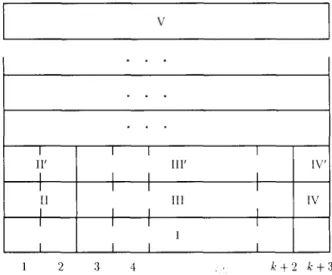
k pebbles, using appropriate dominoes. In a successful tiling, each row (except top and bottom) of the rectangle corresponds to a move made by either player A or B. After a winning move for player A is detected, a white ceiling will then be put on. To gain a better understanding of how this works, consider Fig. 9 in which the tiled rectangle is divided into several regions. Since k is assumed to be odd, odd- (even-) column dominoes will be placed by CONSTRUCTOR (SABOTEUR).

(1) Region I: This is the bottom row of the rectangle, which is used to encode the initial configuration of the pebble game. To be more precise, top(fi+2,1), 1 <i$k, represents the initial location of the ith pebble in G.

. . . . . .

I

. . .

I I I I

II’ III’ IV’

I I I I II 111 IV I I I I 1 I I I I 1 2 3 4 k+2 !i+3

(2) Region II: In this region, CONSTRUCTOR nondeterministically selects a rule for player A.

(3) Region Ill: The dominoes involved in this region are designed to check, by CONSTRUCTOR and SABOTEUR working together in a deterministic way, whether the rule selected in region II is legal or not. Recall that for a rule (x, y, z) to be legal, it must be the case that nodes x and y, but not z, contain tokens in the current pebble game configuration. The outcome will be propagated to region IV.

(4) Region IV: Three cases can happen regarding the selected rule (x,y,z). l Case 1: If (x, y, z) is a legal move and z is not the terminal node, the simulation

continues.

l Case 2: If (x, y, z) is not legal, then a domino whose top color is “B wins” will be placed in this region. As we will see later that our set of domino types does not contain any domino that matches this color, the tiling can never be completed. (SABOTEUR wins in this case.)

l Case 3: If (x, y, z) is legal and z is the terminal node, then a domino with top edge colored “A wins” will be placed in this region. As a result, we can complete the tiling by placing region V on top. (CONSTRUCTOR wins in this case.)

(5) Regions II’, III’ and IV’ are similar to regions II, III and IV, respectively, with the exceptions that in region II ‘, a rule for player B is selected nondeterministically by SABOTEUR, and “A wins” (“B wins”) in cases 2 and 3 above is replaced by “B wins” (“A wins”).

(6) Region I/: This layer can be built iff the last domino of the layer immediately below has its top edge colored “A wins”.

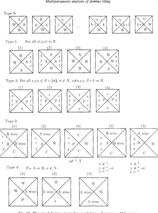
Now we show the detailed construction. The set of domino types involved in the simulation is displayed in Fig. 10. Let S = {si, s2, . , sk} be the set of initial nodes of the pebble game.

Type 0 dominoes are used for constructing the bottom row of the rectangle (i.e., region I). Note that the one and only one applicable domino in the beginning is the leftmost domino of type 0. (This is the only one whose left and bottom edges are colored “white” (“W”).) Once this domino is applied, all the remaining type 0 dom- inoes must be used in the order given in Fig. 10. As a result, the top colors of f3,1&,1, ...> fk+2,1 represent the initial locations of the k pebbles. Also note that ~(fi,i)=A and ro~(f~,~)=B.

In region II, CONSTRUCTOR will pick a move for player A by selecting (non- deterministically) a domino of type 1 (l), for some (x, y, z)ER. Note that at this juncture, there is no way of knowing whether (x, y, z) is legal or not (i.e., whether x and y, but not z, contain tokens). The idea of checking and making (if feasible) the selected move is as follows. First note that the right edge color of the selected domino is “(x, y, z, A)“. Once this domino is put in the plane by CONSTRUCTOR, SABOTEUR has only one choice, namely, using a domino of type l(2) whose left edge matches “(x, y, z, A)“. At this moment, the reader should also note how the top colors of the first two dominoes change (compared to the row underneath), i.e., t~p(f~,~)=B and top( fi, 2) = A. This will allow B’s move to be simulated in the row immediately above.

Multiparameter analysis of domino tiling 211 Type 0: Type :3: (1) (2) (:j) (1) (3)

zf *,

Fig. 10. The set of domino types for simulating a 2-person pebble game

As stated earlier, region III is designed for the purpose of checking whether the selected playing rule is legal or not. This is done by using dominoes of type 2. Suppose that domino f;.-1,2, 3 d i < k + 2, is the one being placed most recently. Consider the following three cases:

(1) Suppose rop(J, I )=x. This implies that node x possesses a token. Hence, the

execution of rule (x, y, z) (if legal) will result in moving a token from x to z. Such a move can be simulated by a domino of type 2(2). Note that top(&)=z and

right(&, 2) = ( * , y, z, A), where * indicates the confirmation of the existence of a token in x.

(2) Suppose top(f;,i)=y. In this case, a domino of type 2(3) will be used. (3) Suppose top(fi,,)=z. In this case, (x, y,z) is not a legal move. A type 2(4) domino (whose right edge color is (x, y, * , A)) will be used to propagate such information to the right.

(4) Suppose top(&)${x, y, z}. Then we simply propagate (x, y, z, A) and top(f;, i) to the right and in the upward directions, respectively, using a domino of type 2(l). Region III is built by CONSTRUCTOR and SABOTEUR in a deterministic way as described above.

Now consider domino fk+3,2 (i.e., the one in region IV). This domino is used to analyze the outcome propagated from region III in order to either continue the simulation or declare a winner. Consider the following three cases:

(1) right(f, + 2,2) = ( * , * , z, A) and z # * or T (the terminal node): In this case, rule (x, y,z) is legal and the pebble game is not over yet. Hence, a domino of type 3(3) (whose top edge color is “C”) will be used to wrap up this row and to allow the simulation to continue.

(2) right(fk+2,2) =( * , * , T, A): This implies that player A’s rule is legal and he first moves a token to the terminal node T. We therefore would like CONSTRUCTOR to be able to finish the tiling in the next run. Color ( * , *, T, A) forces SABOTEUR to utilize a domino of type 3(2) (whose top edge color is “A wins”).

(3) right(f,+ 2,2) # ( * , * , z, A): If this is the case, player A apparently made an illegal move. So we would like SABOTEUR to win. This is done by using a domino of type 3(4) (the only applicable domino at this point).

Suppose that the second row has been completed. We now consider the third row. Suppose t~p(f~+~,*)= C, i.e., neither player A nor player B has won the pebble game. In this case, player B’s move will be simulated by row 3. As we saw earlier that

top(fl,*)= B and t~p(f~,~) = A, CONSTRUCTOR is forced to use a type l(3) domino for fi,3. As a result, SABOTEUR can then nondeterministically select a rule for player B by using a domino of type l(4). (At this point, the reader should pay attention to how alternation between players A and B can be achieved by alternating the top colors of the first two dominoes from row to row.) The checking of the selected rule will be carried out exactly the same way as before by using types 2 and 3 dominoes.

Now we show how the rectangle can be tiled if player A wins. Recall that for all i, top(fk+s,i) is “Cl’, “ A wins” or “B wins”. If “B wins” occurs, then the rectangle can never be finished because of the fact that the right edge of the domino is not white. On the other hand, if “A wins” occurs, then CONSTRUCTOR can use type 4 dominoes to finish the final row of the rectangle. (This is done in a nondeterministic manner. More precisely, in the beginning of each row, CONSTRUCTOR will select a domino from either type 1 or type 4 for fi,i+ 1. If he guesses wrong, then the rectangle will not be completed. Since we are interested in knowing whether there is a winning strategy for CONSTRUCTOR, we may assume that he is “smart” enough to always make the right choice.)

Multiparameter analysis of domino tiling 279 Now, we are able to argue that G has a winning strategy for player A iff CONSTRUCTOR has a winning strategy in the domino game. This is based on the following facts:

l player A’s moves are picked by CONSTRUCTOR, l player B’s moves are picked by SABOTEUR, and

l nondeterminism occurs only in regions II, II’ and the beginning of V.

To complete the proof, it remains to show the size of the domino game. It is easy to see that the numbers of types 0, 1,2,3 and 4 dominoes are bounded by k+3, 3*IR(+l, 8*(JN(+1)4, 2*(1Nj+1)3+2*(INI+1)+2 and INl+3, respectively. Let (N ( = n. The total number of domino types is bounded by O(n4). Since each domino type can be represented in O(log n) bits, the size of the domino problem is bounded by 0(n410gn). Furthermore, the construction can be carried out in 0(n410gZ n) deter- ministic time.

So far we have assumed that k is odd. The simulation for even k is almost identical except that in this case we need an extra column to ensure that dominoes belonging to the first column will always be placed by CONSTRUCTOR. (That is, the total number of columns to be tiled must be even.) The details are left to the reader. Cl Corollary 4.6. The (n, k) 2-person domino game problem requires SZ(n’k-5”‘6-E) deter-

ministic time for any E >O and k> 17, on multitape Turing machines.

Proof. According to Theorem 4.5, the (n, k) 2-person pebble game problem is reduc- ible to the (O(n4), k+ 3) (or (O(n4), k+4), depending on whether k is odd or even) 2-person domino game problem. To derive the lower bound, it suffices to consider the weaker case, i.e., when k is even.

First note that for k> 17, lim,,,(n4 log’n)/(n (k-1)14-E1)=O, for some s1 >O. Now suppose that there exists an O(n (k-5)‘16-E1) deterministic time solution for the (n, k) 2-person domino game problem, for some s1 >O. Since the (n, k) pebble game is

(O(n4 log* n), n4 log n)time reducible to the (n4, k + 3) 2-person domino game, the (n, k)

pebble game problem can therefore be solved in 0(n(k-1)‘4-4ELfE2), for some s1 >O and any c2 >O (according to Lemma 2.3). By picking s2 <4&i, we immediately have that the (n,k) pebble game problem can be solved in 0(n(k-1)14-E), for some E > 0- a contradiction. q

Theorem 4.7. The (n, k) 2-person domino game problem can be solved in O(ncvk)

deterministic time, for some constant c.

Proof. First note that, given an (n, k) 2-person domino game, the number of distinct configurations is bounded by nk. Our result follows immediately from a standard marking procedure, which tries to label each configuration by “yes” or “no” depend- ing on whether a successful tiling can be done if starting in that configuration. A 2-person domino game has a solution iff the initial configuration can be labeled “yes”. 0

Now suppose k is part of the input and is written in the unary notation. Let h be the overall size of an (n, k) 2-person game. Clearly, n, k < h. From Theorem 4.7, the (n, k) 2-person domino game problem can be solved in O(ncrk) deterministic time, for some constant c. This amount is in 0(2c*h*‘og h ) deterministic time. Hence, the (n, k) 2-person domino game problem is in EXPTIME, when k (i.e., the number of columns to be tiled) is a problem parameter. Now consider the lower bound. To show that a problem is EXPTIME-hard, it suffices to reduce a known EXPTIME-hard problem to our problem. To this end, we consider the original 2-person pebble game problem defined and shown to be EXPTIME-complete by Kasai et al. [lo]. Their proof relies on using the 2-person pebble game prob!em to simulate the computation of an arbitrary polynomial space bounded alternating Turing machine. (It is known that the class of languages accepted by polynomial space bounded alternating Turing machines co- incides with EXPTIME.) A careful examination of their proof further reveals that the number of pebbles needed in the simulation is linearly proportional to the amount of space used by the alternating Turing machine. (The reader is referred to [lo] for more details.) This, together with Theorem 4.5, in turn indicates that a p(n) (where p(n) is a polynomial in n) space bounded alternating Turing machine can be simulated by a (O(q(n)),O(p(n))) 2-person domino game (for some polynomial q(n)). Hence we have that the (n, k) 2-person domino game problem is EXPTIME-hard if k is a prob- lem parameter (rather than a fixed constant). (In fact, Corollary 4.6 also reveals the fact that the complexity of the (n, k) 2-person domino game problem is exponential in

k.) Thus, we have the following corollary.

Corollary 4.8. The (n, k) 2-person domino game problem is EXPTIME-complete when

k is a problem parameter written in unary.

The reader should note that when k is part of the input parameter, the problem is exactly the same as the “rectangle tiling game” of [3].

5. An application to concurrent systems

In this section, we show how to use Corollary 4.6 to derive a multiparameter lower bound for the lockout problem of systems of communicating processes. The lockout problem of systems of communicating processes was first considered in [ 111, where it was shown to require Q(c”““* “) time, for some constant c. The size of a system (i.e., n) in [11] was measured solely in terms of the number of bits required to represent the system. Furthermore, the proof of [I l] does not apply to systems with a fixed number of processes. In this section, we will show that for systems of k communicating processes in which the maximum size of each process is bounded by n, the lockout problem requires Q(n(k-7)/16-E) deterministic time, for any E>O and k>21. This, together with an O(ncrk) upper bound, which will also be derived in this section, fully explains how the degree of concurrency (i.e., k) will affect the complexity of the lockout

Multiparameter analysis

of

problem. To be more precise, the problem is solvable in polynomial time if the number of processes is a fixed constant. However, the degree of the polynomial grows linearly as the number of processes increases. If the number of processes is not fixed, then the problem becomes EXPTIME-complete. In what follows, we give an informal defini- tion of the lockout problem. The reader is referred to [l l] for formal definitions of communicating processes and the lockout problem.

A communicating process P is a directed labeled graph (V, E), where I/ (the set of vertices) and E (the set of edges) represent the sets of states and transitions, respect- ively. Each transition (edge) of a process is labeled by a two-tuple [i, c], where i is a process name and c is a message type. A system of communicating processes P is an n-tuple (PI, P2, . . . . P,,), where each Pi is a process. A state of P is an n-tuple

(ql, q2, . . , qn), 1 <i < n, where qi is a state of process Pi. The communication between processes is synchronized by the notion of “hand-shaking”. If at any one time, two processes A and B are in states p and q, respectively, and p % p’ and q ‘A’c1 -4’ are two transitions from states p and q, respectively, then processes A and B can communicate with each other by exchanging message c and simultaneously enter states p’ and q’, respectively. The size of a process is defined to be the size of its graph representation when a standard binary encoding scheme is used.

A process, say P, is locked out of a predefined set of states Q if regardless of how hard it tries to move towards Q, the remainder of the system can always “conspire” in such a way as to prevent P from entering Q. The lockout problem is that of determining whether a process is locked out of a set of states in a given system. See [ 1 l] for a more detailed definition of the lockout problem. Let %(n,k) be the class of systems of

k communicating processes in which the size of each process is bounded by n. Now we are in a position to show our lower bound result.

Theorem 5.1. The lockout problem for W(n, k) requires Cl(n (k-7)/16-E) deterministic time,

for any E>O and k>21.

Proof. The proof relies on showing that, given an (n, k) 2-person domino game, we can construct a system of communicating processes in %‘(n log n, k + 2), a process P and a set of states Q in such a way that the domino game has a winning strategy for CONSTRUCTOR iff P is not locked out of Q.

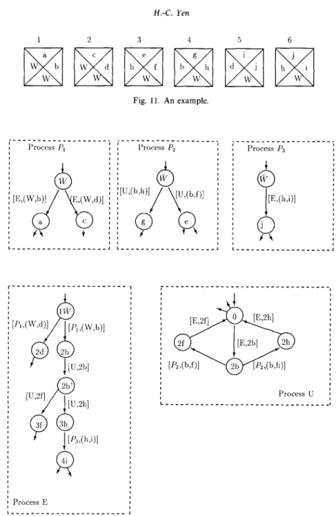
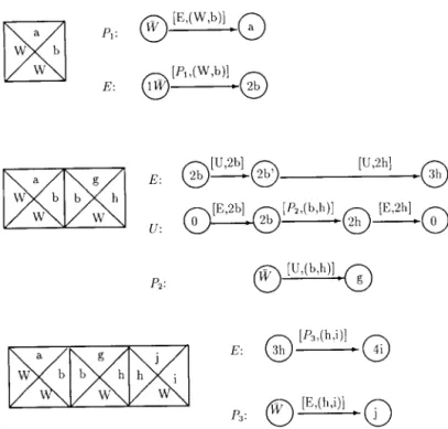
We begin by using a simple example to illustrate the first few steps of the simulation so as to allow the reader to have a better understanding of the proof. In this example, we assume that the width of the region to be tiled is 4. Now consider the set of domino types displayed in Fig. 11. The associated system is shown in Fig. 12.

The intuition behind the simulation is to use a process Pi, 1~ i < 4, to simulate row

i of the tiling, and two additional processes E and U to simulate CONSTRUCTOR and SABOTEUR moves, respectively.

Initially, all processes Pi’s are in state Wand processes E and U are in states 1 @and 0, respectively. Figure 13 illustrates the first 3 moves of the simulations. More precisely, these are as follows.

Fig. 11. An example. “ _ _ _ _ _ _ _ _ _ _ _ _ _ _ _ ‘ _ _ . , i______----_________. 9 l’roccss PI Process Pz I : : 8 --____-____----_--_. Process P3 I I I I j Process E I _I L____-__________________ 1

Fig. 12. A concurrent system for the example in Fig. 11.

(1) Simulation of the jifirst domino: CONSTRUCTOR begins by placing either a type 1 or type 2 domino in the lower left-hand corner. Suppose a type 1 domino is picked. This will be simulated by the exchange of message (W, b) between processes PI and E. (Likewise, the exchange of message (W, d) will correspond to the selection of

Multiparameter analysis of domino tiling 283

P*:

[k(h>i)l E:

0

0

PJ:

0

rv

[WWI c j

0

Fig. 13. Simulation of the first three dominoes.

a type 2 domino.) The subsequent states of P1 and E are a and 2b, respectively. The meanings of a and 2b deserve further explanation. Since the chosen domino is of type (W, b, W, a), colors a and b have to be recorded in order to match the dominoes on top and to the right. This is accomplished by using the finite state controls of processes Pi and E to record the top and right colors of the domino, respectively. In addition, the column number to be tiled next is also kept in E’s finite-state control.

(2) Simulation of the second domino: Since SABOTEUR’s job is to prevent CONSTRUCTOR from completing the tiling, it is therefore needed to “force” E to do whatever SABOTEUR does. Thus, we would not let E communicate with P2 directly. Instead, E must first communicate with U through the exchange of message 2b. One may think of 2b as a wake-up call, initiating the communication between U and Pz. (Note that this is the only available move in the entire system at this point.) SABOTEUR has two choices for the second domino (type 3 or 4). Suppose SABOTEUR picks type 4. This will be simulated by U and Pz through the exchange of message (b, h). (Subsequently, U and P2 will enter states 2h and g, respectively.) At this point, the only feasible move is for E to enter state 3h (from 2b’) by exchanging message 2h with U. (Note that E’s move is ‘forced” by the previous moves of U and Pz .) It is worth mentioning that E has no control of what U and P2 will do. As a result, U and Pz can conspire in a way that E will not be able to enter its desired set of states. (At this moment, the reader should pay special attention to the nondeterministic choice in state 2b of process U.)

(3) Simulation of the third domino: similar to that of the first move.

Now, given a set of domino types T, we construct the following system of com- municating processes:

(1) PROCESS Pi=(K:,Ei), l<idk:

0 K = { W) u Color(T), 0 Ei contains:

(a) w [JC CL*)1

- t if (l, r, W, t)~ T and i is odd (“V’ must be W for i= 1). [E. (1% r)l

(b) b-

- t if (I, r, W, t)~ T and i is even (“r” must be W for i = k),

(4 b-

(4 W-

[E,pll

(2) Process E = ( vE, E’):

0 VE={lW,s}u(ix,ix’ll~i~k, x~Color(T)}u{iq/1<16k}, where s,q are not in

Color(T), a E’ contains:

(a) 1 WIPI.wJr)l

- 2r if (W, r, W, t)E T, for some t, IPi, (I.*)1

(b) il- (i @ 1)r if (I, r, b, t)E T, for some t, b, and i is odd,’ [U, ill

(c) il- il’ if i is even,

(d)

il,z

(i @ l)r, i is even,

(e) lW[p’.2q,

(f) iq- [P”hl(i+l)q, 2<i<k-1, (g) kq ‘2) s.

(3) Process U = ( Vu, ELI):

l VU= (0) u {ix 1 xECoIor(T), i is even}, 0 EU contains (for all even i):

(4 O- tE’ifl il, V’1EColor(T),

Multiparameter analysis of domino tiling 285

[P.,(L*)I

(b) il- ir if (1, r, b, t)~ T, for some t, b,

(c) ir- ‘E’irl 0, Vr~Color(T).

We define a system configuration to be (cl, . . . . ck,e, u), where ci is a state of Pi, for 1 did k, e and u are states of E and U, respectively. We claim that process E is not locked out of {s) iff the domino game has a winning strategy for CON- STRUCTOR. This claim relies on the following facts:

(1)

(2)

((C1,,Ci-l(,di-1,ct,...,~k) is a reachable domino configuration iff (c 1, . . , ci_ 1) Ci, . . .) Ck, idi_ 1) 0) is a reachable system state.

Consider the following configuration change as a result of placing domino d: (Assume that d=(di- 1) di, Ciy C:).)

((C1,,Ci_llrd,c, . ..> cr)-(M],d>c, .,.,G);

(a) if i is odd, d will be simulated by

(b) if i is even, d will be simulated by

(1) [U,id;-11 E idi_I-id;_I (2) (3) [U,idil id{_l-idi u O-idi_, [E, id, - I 1 idi- [Pi,(d,-l.d,)l b idi idi- tE, id;1

pi

[L’,(di-l-&)1

ci FC;

and nondeterminism occurs only in (2).

(3) Process E can reach s iff (-1, W ) is a reachable domino configuration.

Facts 1 and 2 can easily be proved by induction on the number of domino moves. Fact 3 is quite obvious. As a result of facts 1-3, the domino game has a winning strategy for CONSTRUCTOR iff process E is not locked out of state s in the constructed system.

Now we analyze the size of the system. Clearly, the sizes of Pi, E and U are all bounded by O(n log n) and the construction can be carried out in O(n log2 n) deter- ministic time. As a result, the (n, k) 2-person domino game problem is reducible to the lockout problem for systems in %?(n log n, k + 2) with respect to (n log2 n, n log n)rime reducibility. We also know from Corollary 4.6 that the (n, k) 2-person domino game

problem requires !S(n (k-5)‘16-E) deterministic time, for

17. Thus, if the lockout

problem for systems in %?(a,

were solvable in II (k- ‘)/r6-” deterministic time, for

some e1 >O, then according to Lemma 2.3 the (n,

2-person domino game problem

would be solvable in (,logn)“k+2’-7”‘6-“’

d e erministic

t

time, for

21. (To apply

Lemma 2.3, we require that nlog* ~~~(nlogn)“~‘~‘-‘“‘~-‘~,

which holds if k>21.)

The above amount is in n(k-5)/16+E2-E1

deterministic time, for any s2 > 0. By letting

E2<Et, we

have that the (n, k) 2-person domino game problem can be solved in

n(k-5)‘16-E3 deterministic time, for some s3 >O - a contradiction. This completes the

proof.

0

Now the upper bound.

Theorem 5.2. The lockout problem for %?(n, k) can be solved in O(nc*k) deterministic time, for some constant c.

Proof.

Since the total number of distinct global states for any system in

is

bounded by

the result can be proved by using the labeling algorithm described

in [ll].

Acknowledgment

The author thanks the anonymous referee for numerous suggestions that greatly

improved the presentation as well as the correctness of this paper.

References Cl1

PI

A. Adachi and S. Iwata, Some combinatorial game problems require Q(nk) time, J. ACM, 31 (2) (1984) 361-376.

R. Berger, The undecidability of the domino problem, Mem. Amer. Math. Sot. 66 (1966) B. Chlebus, Domino-tiling games, J. Comput. System Sci. 32 (3) (1986) 374-392.

B. Chlebus, Proving NP-completeness using bounded tiling, J. Inform. Process. Cybernet. EIK, 8 (1987) 479-484.

E. Gradel, Domino games with an application to the complexity of Boolean algebras with bounded quantifier alternations, in: Proc. Symp. Theoretical Aspects of Computer Science (1988) 98-107. D. Hare], Recurring dominoes: making the highly undecidable highly understandable, Ann. Discrete Math. 24 (1985) 51-72.

D. Hare], Effective transformations on infinite trees, with applications to high undecidabihty, dominoes, and fairness, J. ACM, 33 (1) (1986) 224-248.

J. Hopcroft and J. Ullman, Introduction to Automata Theory, Languages, and Computation (Addison- Wesley, Reading, MA, 1979).

T. Kasai and S. Iwata, Gradually intractable problems and nondeterministic log-space lower bounds, Math. Systems Theory, 18(2) (1985) 153-170.

T. Kasai, A. Adachi and S. Iwata, Classes of pebble games and complete problems, SZAM J. Comput. 8 (4) (1979) 574-586.

Multiparameter analysis of domino tiling 287

[I I] R. Ladner, The complexity of problems in systems of communicating sequential processes, J. Comput. System Sci. 21 (1980) 179-194.

1121 H. Lewis, Complexity of solvable cases of the decision problem for the predicate calculus, IEEE FOCS (1978) 35-47.

[13] H. Lewis and C. Papadimitriou, Elements of the theory of computation (Prentice-Hall, Englewood Cliffs, NJ, 1981).

1141 L. Rosier and H. Yen, A multiparameter analysis of the boundedness problem for vector addition systems, J. Comput. System Sci. 32 (1) (1986) 105-135.

[IS] L. Rosier and H. Yen, On the complexity of deciding fair termination of probabilistic concurrent finite-state programs, Theoret. Comput. Sci. 58 (1988) 263-324.

[16] M. Savlsberg and P. van Emde Boas, Bounded tiling, an alternative to satisfiability? in: Proc. 2nd Frege Conference, Schwerin (1984); Mathematische Forschung 20 (1984) 354-363.

1171 J. Seiferas, Techniques for separating space complexity classes, J. Comput. System Sci. 14 (1977) 73-99. [18] P. van Emde Boas, Dominoes are forever, in: Proc. 1st GTI Workshop, Paderborn (1983) 76-95. [19] H. Wang, Proving theorems by pattern recognition ii, Bell System Tech. J. 40 (1961) 1-4.

1201 H. Yen, Communicating processes, scheduling and the complexity of nontermination, to appear in Math. Systems Theory.