國立臺灣大學理學院應用數學科學研究所 碩士論文
Institute of Applied Mathematical Sciences College of Science
National Taiwan University Master Thesis
運動賽事期間隊伍能力的變化分析
Analyzing Dynamic Abilities of Teams in Sports Events
管敏仁 Min-Ren Guan
指導教授:江金倉 博士
Advisor: Chin-Tsang Chiang, Ph.D.
國立臺灣大學碩士學位論文
口試委員會審定書
-� 動賽事期間隊伍能力的變化分析
nalyzing Dynamic Abilities of Teams in Sports Event
論文亻系嵒敏仁君(R07246013)在國立全滑大學教學學系、所 完成之碩士學位論文 ,於民國109年7月22日承下列考拭委員-L -=
面過及口讠式及格,特此證明
口試委
5L仝定 (簽名)
4 勺巨
L
、h�., ,,
系主任 、所表 (簽名)
(走否須簽幸依各院系所規定)
中文摘要
在成對比較類型的運動數據分析中,實務工作者和研究者們認知球隊在連續 比賽中,由於受傷、團隊心理和團隊進步會導致團隊能力變化。描述分數差或比賽 結果最常用的框架主要是對主場隊伍和客場隊伍的能力差做適當的轉換。在這樣 的考慮下,隊伍能力的變化可以在頻率派學者或貝氏的觀點下進一步建模。通過整 合這些特點到模型的構造中,我們對團隊能力提出更通用的動態模型。此外,我們 還制定了一些準則來從競爭模型中選出擁有較好季後賽預測力的模型。我們透過 美國國家籃球協會 2009-2010 賽季到 2018-2019 賽季的數據來調查提案的實用性。
關鍵字:成對比較、動態能力、混合效應模型、模型選擇、預測率、預測均方差
Abstract
In paired-comparison sports data analysis, practitioners and researchers have iden- tified the varying abilities of teams due to injuries, team psychology, and team improvement in the course of sequential competitions. The most commonly used framework to describe the score difference or the match outcome is mainly based on an appropriate transformation of the difference in abilities of the home team and the visiting team. Under such consideration, the abilities of teams can be fur- ther modelled with dynamic effects in the frequentist or Bayesian perspective. By integrating these features into a model formulation, we propose more general dy- namic models for the abilities of teams. In addition, some criteria are developed to select a better predictive model for playoffs among competing models. The practicality of our proposal is also investigated by the data from the 2009-2010 season to the 2018-2019 season of the National Basketball Association.
KEY WORDS: Paired comparisons; Dynamic abilities; Mixed effects models;
Model selection; Proportion of correct predictions; Prediction mean squared er- ror.
Contents
Abstract i
List of Figures iii
List of Tables iv
1 Introduction 1
2 Existing Paired Comparison Models 3
3 Proposed Models for Dynamic Effects 5
3.1 Background . . . 5 3.2 Regression Model Formulation . . . 8
4 Estimation and Model Selection 10
4.1 Estimation . . . 10 4.2 Model Selection . . . 12 5 An Application to National Basketball Association 14
6 Conclusion and Discussion 16
List of Figures
6.1 Proportion of correct predictions of M·PCP (red line), M·PMSE
(blue line), andM·BIC(green line). Black lines are the highest and lowest proportions of correct predictions amongM·for· = 1, 2, and T . . . . 20 6.2 Selected plots of minimized sum of squares value to λ. . . 22 6.3 Selected plots of minimized sum of squares value to λ. . . 22
List of Tables
6.1 The estimated proportion of correct predictions from the Dynamic Bradley-Terry models (cf. [6]) and the selected proposed models on playoffs data.. . . 21 6.2 Mean of proportion of correct predictions of Dynamic Bradley-
Terry model (cf. [6]) and proposed models over the ten seasons. . 22 6.3 Ratio of ˆσh2 to ˆσ02 and ˆσh2 to ˆσ02(rounded to 3 decimal places) . . . 23 6.4 Mean of PCP and BIC over ten seasons . . . 24
Chapter 1 Introduction
How to assess abilities of sports teams has been of great interest to researchers and practitioners. National Collegiate Athletic Association (NCAA) established a ranking system reflecting the abilities of teams to select teams for playoffs. Pre- dictions of future outcomes can be made by the abilities of participating teams, which are highly concerned by practitioners.
Paired comparison models have been commonly used for sports events. A sea- son of basketball matches in NBA league can be regarded as a series of paired comparisons. The advantage of paired comparisons is reducing the effects of con- founding. For example, two teams share the same referee in a match, whereas one team may played with several different referees throughout the whole season and there may be judgement biases among referees. Existing Paired comparison mod- els for sports events characterize the score difference or outcome to be related with home team’s ability and visiting team’s ability by a linear model or generalized linear model respectively.
Previous studies proposed a variety of paired comparison models for sports events including random/fixed effects models with/without dynamic effects on the abilities. In the spirit of existing models, we further propose two flexible models under different cases and many of existing models can be unified in the proposed models. We connect Bayesian and frequentist viewpoints by mixed effects models.
1. Introduction 2
The dynamic scheme of abilities is more general by considering fixed dynamic scheme and random processes for the abilities simultaneously. We provide model selection criteria to select a better model and setup for the prediction purpose. Two measures of predictive ability are used to compare the predictive performances of competing models.
In section 2, several existing paired comparison models are introduced. Sec- tion 3 describes the proposed models under different setups. Section 4 intro- duces the estimation method, which consists of least squares method, maximiz- ing observed likelihood, and maximizing posterior likelihood. The measures of goodness-of-fit and predictive ability are also introduced. Section 5 presents an application to the National Basketball Association.
Chapter 2
Existing Paired Comparison Models
Let m be the number of matches; T the number of teams; Yithe score difference of match i, i = 1, . . . , m; akand bkthe home ability and visiting ability of team k respectively, k = 1, . . . , T ; hi and vithe home team and visiting team in match i respectively; and tithe time of match i.
The first paired comparison model for sports events proposed by [1] did not consider the dynamic effects and the home ability and visiting ability were con- sidered to be the same. That is, ak = bk , αk,∀i = 1, . . . , m, and k = 1, . . . , T , which leads to the following model:
Yi = αhi− αvi+ εi, i = 1, . . . , m. (2.1) [2] improved model (2.1) by considering the home court advantage θ, i.e.,
ak, αk+ θ and bk , αk, which leads to the following model:
Yi = θ + αhi− αvi+ εi, i = 1, . . . , m. (2.2) [3] considered team-specific home court advantages θk, i.e., ak , αk + θk and bk , αk, which leads to the following model:
Yi = θhi + αhi − αvi+ εi, i = 1, . . . , m. (2.3) The first model considering the dynamic abilities was proposed by [4]. The model suggested that there is a deviation of performance Sk(ti) from a team’s
2. Existing Paired Comparison Models 4
underlying ability in each game. In the formulation of (2.2), let ak(ti), θ+αk(ti) and bk(ti), αk(ti). The model leads to
αk(ti) = αk+ Sk(ti), (2.4) where Sk(ti) follows a random process. [5] proposed a model for ordered cate- gories:
P (Yi ≤ r) = F (θr+ αhi(ti)− αvi(ti)), r = 1, . . . , k (2.5) with αk(ti) following a random process and αk(0) = αkfor all k. [4] and [5] both assumed that the dynamic effects on ability depends on some random processes, wheras [6] proposed a fixed dynamic scheme for the dynamic evolution of ability.
Let λ1, λ2 ∈ [0, 1] and Yi = 1 if the home team won, and Yi = 0 if the visiting team won. t(i−1) denotes the time of the previous home match in which hi was also the home team, t′(−1)i denotes the time of the previous away match in which vi was also the visiting team. [6] proposed the following dynamic Bradley-Terry model:
P (Yi = 1|Yi−1 = yi−1, . . . , Y1 = y1) = exp{ahi(ti)− bvi(ti)} 1 + exp{ahi(ti)− bvi(ti)}
with
ahi(ti) = λ1γ1y(t(i−1)) + (1− λ1)ahi(t(i−1)), bvi(ti) = λ2γ2(1− y(t′(−1)i )) + (1− λ2)bvi(t′(−1)i ),
(2.6)
where y(ti) denotes the outcome of the match at time ti. [6] assumed that all teams started with the same home and visiting underlying abilities γ1r¯h and γ2r¯v respectively, where ¯rhand ¯rvare the average win rates of home matches and away matches over the previous regular season respectively.
Chapter 3
Proposed Models for Dynamic Effects
Based on existing models, a paired comparison model for sports events can be formulated as
Yi = ahi(ti)− bvi(ti) + εi, i = 1, . . . , m. (3.1) The main issue is how to model the dynamic evolutions of abilities ahi(ti) and bvi(ti) for i = 1, . . . , m. Let Yi denote the score difference of match i. Yh(ti) and Yv(ti) denote the scores of the home team and the visiting team of match i respectively. For the regression formulation, we define the following notations:
Y =
Y1
... Ym
, ε =
ε1
... εm
, a =
a1
... aT
, b =
b1
... bT
, γ1 =
γ11
... γ1T
, and γ2 =
γ21
... γ2T
.
3.1 Background
In the spirit of [6], we propose a more general model for abilities (hereinafter referred to M1):
ahi(ti) = λ1γ1hiyh(t(i−1)) + (1− λ1)ahi(t(i−1)), bvi(ti) = λ2γ2viyv(t′(−1)i ) + (1− λ2)bvi(t′(−1)i ).
(3.2)
3. Proposed Models for Dynamic Effects 6
The underlying abilities akand bkare fixed unknown parameters for k = 1, . . . , T . The dynamic Bradley-Terry model is a special case of model M1 under the fol- lowing three conditions: (i) underlying abilities are set to be the average win rates of home matches and away matches over the previous regular season respectively.
(ii) γ11 = · · · = γ1T and γ21 = · · · = γ2T. (iii) The score difference is replaced with the outcome.
In model M1, the underlying abilities a and b are involved in the updating scheme with scores. Thus the effects of underlying abilities will decrease as the season goes on. However, model (2.4) provides a different aspect: The effects of underlying abilities should be the same throughout the season. The dynamic effects are explained as the deviations of the actual performances from the underly- ing abilities. Considering the feature, we propose a model in which the underlying abilities are not involved in the updating scheme (hereinafter referred to M2):
ahi(ti) = ahi+ γ1hiShi(ti) and bvi(ti) = bvi+ γ2viSvi(ti), Shi(ti) = (1− λ1)Shi(t(i−1)) + λ1yh(t(i−1)),
Svi(ti) = (1− λ2)Svi(t′(−1)i ) + λ2yv(t′(−1)i ),
(3.3)
where Svi(0) = 0 and Shi(0) = 0.
There are two meaningful cases of model M2: λ1 = λ2 = 1 and λ1 = λ2 = 0 (hereinafter referred to M2-i and M2-ii respectively). The former implies that the dynamic effects only count on the result of the previous match. That is,
Shi(ti) = yh(t(i−1)) and Svi(ti) = yv(t′(−1)i ). (3.4) The case of λ1 = λ2 = 0 means that there is no dynamic effect, i.e.,
S (t )≡ 0 and S (t )≡ 0. (3.5)
3. Proposed Models for Dynamic Effects 7
Above models are in the frequentist framework, the abilities are updated by fixed parameters and historic data. In Bayesian framework, the abilities are up- dated by some random processes. The simplest case is the first-order random
walk model:
ahi(ti) = ahi(t(−1)i ) + uh(ti), bvi(ti) = bvi(t′(−1)i ) + uv(ti),
(3.6)
where uh(ti)’s i.i.d.e N (0, σh2), uv(ti)’s i.i.d.e N (0, σv2) and they are mutually inde- pendent for i = 1, . . . , m. Considering both factors simultaneously, we further propose models M1R, M2R, M2R-i and M2R-ii from M1, M2, M2-i and M2-ii re- spectively, in which the abilities follow a random process. In the case of first-order random walk, M1R and M2R are proposed as the follows respectively.
ahi(ti) = λ1γ1hiyh(t(i−1)) + (1− λ1)ahi(t(i−1)) + uh(ti), bvi(ti) = λ2γ2viyv(t′(−1)i ) + (1− λ2)bvi(t′(−1)i ) + uv(ti).
(3.7)
ahi(ti) = ahi+ γ1hiShi(ti) and bvi(ti) = bvi+ γ2viSvi(ti), Shi(ti) = (1− λ1)Shi(t(i−1)) + λ1yh(t(i−1)) + uh(ti),
Svi(ti) = (1− λ2)Svi(t′(−1)i ) + λ2yv(t′(−1)i ) + uv(ti).
(3.8)
The underlying abilities a, b and parameters of dynamic effects γ1, γ2 can be fixed unknown parameters or random parameters. From frequentist viewpoint, if the sample size is large enough, consistency of the estimation guarantees the esti- mated parameters will converge to the true parameters. Form Bayesian viewpoint, by assuming the parameters follow some prior distributions, it can reduce the num- ber of parameters to be estimated, which is an advantage when the sample size is small. We cover above two viewpoints by considering the following 4 different cases:
Case 1 . a, b and γ1, γ2 are fixed;
Case 2 . a, b are fixed and γ1, γ2are random;
Case 3 . a, b are random and γ1, γ2are fixed; and
3. Proposed Models for Dynamic Effects 8
Case 4 . a, b and γ1, γ2 are random.
In each of above cases, if a and b are random, we assume that ak’s i.i.d.e N (µa, σ2a) and bk’si.i.d.e N (µb, σb2). If γ1and γ2are random, we assume that γ1k’s i.i.d.e N (µ1, σ12) and γ2k’s i.i.d.e N (µ2, σ22) and all the random parameters are mutually independent.
If there is any random parameters, the normality assumption εi’s i.i.d.e N (0, σ20) is required due to concerns about estimation.
3.2 Regression Model Formulation
All proposed models can be rewritten as the following form:
Y = Xβ + ε, (3.9)
where
β =
a b γ1 γ2 uh uv
with uh =
uh(t1) ... uh(tm)
, and uv =
uv(t1) ... uv(tm)
.
Model M1 is chosen as an example to show how to obtain the regression formula- tion. In an arbitrary match i (or at time ti), the home ability and visiting ability of team hi and team viunder model M1 can be rewritten as the follows respectively:
ahi(ti) = (1− λ1)K1ahi+hλ1PKj=01−1(1− λ1)jyh(t(i−j−1))iγ1hi, bvi(ti) = (1− λ2)K2bvi+hλ2PKj=02−1(1− λ2)jyv(t′(−j−1)i )iγ2vi,
(3.10)
3. Proposed Models for Dynamic Effects 9
M2R, M2R-i and M2R-ii. If there are random effects in the model, mixed effects model formulation has more advantages in estimation.
Let βR denotes the random parameters and βF denotes the fixed parameters, i.e.,
Case 2. βR =
γ1− µ11T
γ2− µ21T
, βF =
a b µ1 µ2
;
Case 3. βR=
a− µa1T
b− µb1T
, βF =
µa
µb γ1
γ2
; and
Case 4. βR=
a− µa1T
b− µb1T
γ1− µ11T
γ2− µ21T
, βF =
µa µb µ1 µ2
.
Due to the problem of identifiability, we assume that µb = 0 in model M2, M2-i, M2-ii, M2R, M2R-i and M2R-ii. By similar procedures, one can derive the mixed effects model formulation:
Y = XRβR+ XFβF + ε. (3.11)
Chapter 4
Estimation and Model Selection
To write down the estimation approach explicitly, we first define some notations.
Let Xγ1 and Xγ2 be the covariate matrix of γ1 and γ2 respectively. Let γ = (γ1T, γ2T)T, Xγ = (Xγ1, Xγ2), and Y∗ = Y − XFβF.
4.1 Estimation
By the model formulation (3.11):
Y = XRβR+ XFβF + ε, XFβF + ε∗, (4.1) where ε∗ = ε + XRβRand ε∗ ∼ Nm(0, σ20Im+ XRV ar(βR)XRT). The estimation approach of βF and λ is proposed to minimize the sum of squares
SS(λ, βF) = (Y − XFβF)T(Y − XFβF). (4.2) Least square method can be applied in this minimization.
minλ,β SS(λ, βF) = min
λ min
β SS(λ, βF) = min
λ (Y − XFβˆF)T(Y − XFβˆF),
4. Estimation and Model Selection 11
where Σ = σ02Im+ σ12Xγ1XγT1 + σ22Xγ2XγT2 and the observed log-likelihood func- tion is
−m
2 log(2π)−m
2 log σ20−1
2log|Im+ σ21
σ20Xγ1XγT
1 + σ22
σ20Xγ2XγT
2|
− 1
2σ02(Y − XFβF)T(Im+ σ21
σ20Xγ1XγT1 +σ22
σ02Xγ2XγT2)−1(Y − XFβF).
(4.4)
The estimation approach for (σ02, σ21, σ22) is proposed to maximize the observed log-likelihood function, i.e.,
(ˆσ02, ˆσ21, ˆσ22) = argmax
(σ20,σ12,σ22)
l(σ20, σ12, σ22|X, Y ).
To estimate the predictors ˆγ1 and ˆγ2 of γ1 and γ2, it is proposed to maximize the posterior log-likelihood. That is,
ˆγ1 ˆ γ2
= argmax
(γ1,γ2)
log L(γ1, γ2|ˆσ20, ˆσ12, ˆσ22, X, Y ), (4.5)
where
log L(γ1, γ2|σ02, σ12, σ22, X, Y )∝ log fY(y|σ02, γ1, γ2)π(γ1, γ2|σ21, σ22)
= −m
2 log(2π)−m
2 log σ02− 1
2σ02|(Y − XFβF − Xγ1γ1+ Xγ2γ2)|2 (−m) log(2π)−m
2(log σ21 + log σ22)− 1 2( 1
σ12|γ1|2+ 1 σ22|γ1|2)
∝ −(Y∗− Xγγ)T(Y∗− Xγγ)− γTW γ,
and
W =
σ02
σ12IT 0 0 σ02
σ22IT
.
The posterior log-likelihood is maximized when
γˆ1 ˆ γ2
= (XγTXγ+ W )−1XγTY∗ = E[γ|σ21, σ22, σv2, X, Y ]. (4.6)
4. Estimation and Model Selection 12
4.2 Model Selection
With all the models and cases, how to select the best model is an important is- sue. Good predictions of outcomes and difference in scores are important for practitioners. In the following paragraphs, we first introduce two measures of pre- dictive ability to measure the performance of a model on the prediction purpose.
Then several criteria are proposed based on goodness-of-fit and predictive ability measured by regular season data.
The measures of predictive ability are proportion of correct predictions and prediction mean squared error, hereinafter denoted by PCP and PMSE respec- tively. Let (X0, Y0) be a future run.
PCP(M) = P (sign(Y0)· sign(X0βˆM) > 0) + 0.5P (X0βˆM = 0), (4.7) and
PMSE(M) = E(Y0− X0βˆM)2, (4.8) where ˆβM denotes the estimate of β under modelM. To estimate the PCP and PMSE of modelM, the playoffs data are considered as future runs and the prob- ability is estimated by the empirical distribution of playoffs data.
The Bayesian Information Criterion in [7] is a common approach in model selection. With the observed log-likelihood function (4.4), the BIC value of a modelM is derived by
BIC(M) = −2 log L(M) + pMlog m, (4.9) where pM denotes the number of parameters in the modelM. [7] suggested to choose the model with smallest BIC value.
4. Estimation and Model Selection 13
by applying the estimated parameters to the testing data. To be more explicit, we introduce the following notations:
Y =
Ytr Yte
, X =
Xtr Xte
,
where (Xtr, Ytr) and (Xte, Yte) denote the training data and testing data respec- tively. Let ˆβMtr be the estimate of β by the training data under modelM. The PCP and PMSE of modelM are estimated by
PCP(d M) = 1 S
XS i=1
h
I(sign(Yite)· sign(XiteβˆMtr) > 0) + 0.5I(XiteβˆMtr = 0)
i
, (4.10) and
PMSE(\ M) = 1 S
XS i=1
(Yite− XiteβˆMtr)2, (4.11) where S is the number of matches in testing data. The modelMPCP andMPMSE
with highestPCP and smallest \d PMSE are chosen, i.e., MPCP = argmax
M
PCP(d M) (4.12)
and
MPMSE = argmin
M PMSE(\ M). (4.13)
Chapter 5
An Application to National Basketball Association
The proposed models are applied to 2009–2010 season to 2018–2019 season of National Basketball Association. The data are available via an API provided in [8].
The data consist of the index of every match sorting by calendar time, the home teams and visiting teams of every match, and scores of the home teams and away teams in every match. The regular season is used to fit the proposed models and the playoffs data are treated as future runs to estimate the proportion of correct predictions and prediction mean squared error. Model M1 and M2 with λ ∈ Λ are also considered in this section, where Λ = {k(0.1, 0.1)T : k = 0, . . . , 9}.
Hereinafter we denoteM· = {M · including the cases λ ∈ Λ}, for · = 1, 2, and MT =M1∪ M2.
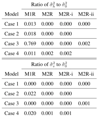
We investigate the dynamic effects of abilities in model M1R, M2R, M2R-i and M2R-ii with first-order random walk. The means of the ratios ˆσh2/ˆσ20 and ˆ
σ2/ˆσ2 over ten seasons are shown in Table6.3. In these NBA data, the variances
5. An Application to National Basketball Association 15
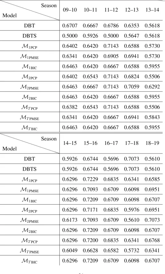
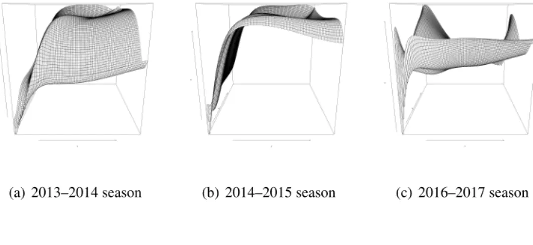
The proportion of correct predictions of dynamic Bradley-Terry model (2.6) proposed in [6] (hereinafter referred to DBT model) and its modification which replaces the outcome with score difference (hereinafter referred to DBTS model) are listed in table6.1compared to the proposed models. DBT model produces pre- dictions that the home team will win for every match. DBTS model has lower PCP than the proposed models. One step of estimating the parameters is to minimize the sum of squares function (4.2). Figure6.2and6.3show that the non-convexity of sum of squares function under model M1 and M2 makes the minimization dif- ficult. Thus we do not recommend DBT model and DBTS model.
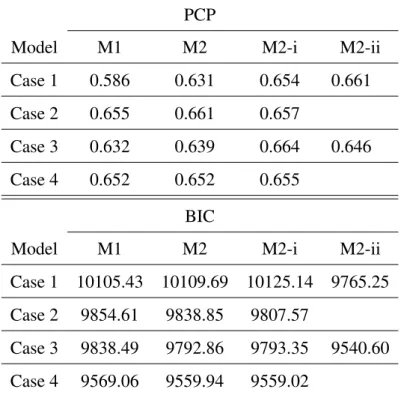
Table6.4shows the mean of BIC values over ten seasons under different mod- els and cases. BIC suggests that model M2-ii in the case that abilities are random should be selected, which means that there is no dynamic effect. The conclusion also holds if we look at the BIC values season by season.
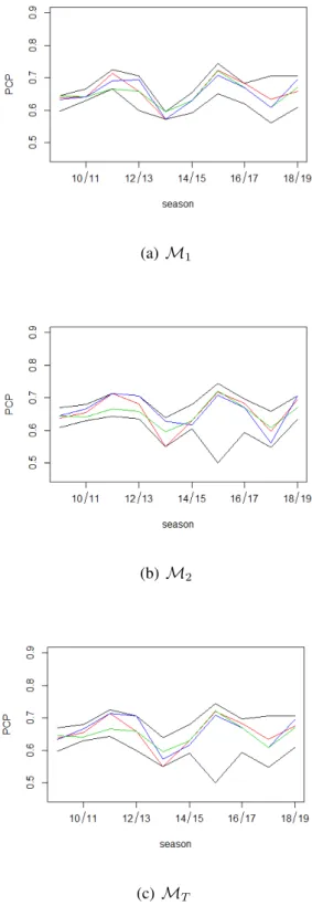
We compare the PCP of MPCP, MPMSE and model MBIC (without dynamic effect) for ten seasons to see if there is an evidence of dynamic effect. In most of the seasons except 2015-2016 season, the models with dynamic effects can have higher PCP than model MBIC. This can be an evidence that there are dynamic effects in most of the seasons except 2015-2016 season. Moreover, in 2010–2011 season to 2012-2013 season we successfully select the models with dynamic effect with higher PCP than model MBIC. Over the ten seasons, the PCP of selected models are comparable to the highest PCP of all models except 2013-2014 season and 2017-2018 season.
Table 6.4 shows the mean of PCP’s over ten seasons under different models and cases. We can see that most of the models are comparable except model M1 under case 1, M1 under case 3, and model M2 under case 2.
Chapter 6
Conclusion and Discussion
In the application to NBA, table6.2shows that the fixed dynamic scheme inspired by [6] performs poorly in the sense of prediction with PCP 0.586 and DBT model tends to produce meaningless predictions that the home team always wins. Es- timation of the weight λ is also difficult (see Figure6.2) and such estimation is based on the sense of goodness-of-fit, which may not correspond to the predictive ability. The fact that uh and uv are inapparent shows that the first-order random walk assumption on the home ability and visiting ability (cf. [4] and [5]) has no contribution to the dynamic effects. To sum up, most of the existing approaches to estimate the dynamic effects are based on the goodness-of-fit with some specific models. By such approaches, either there is no evidence of dynamic effects or the dynamic effects may produce poor predictions.
In the aspect of regression, λ should play the role as designed covariate. As- signing given values to λ avoids the difficulties in estimation and the proposed model selection criteria can suggest the best λ in the sense of predictive ability.
In the applications to NBA, the proposed model selection criteria can select the
6. Conclusion and Discussion 17
better. In the applications to NBA, the format of playoffs and regular season are different, which may decrease the PCP and increase PMSE for our models. This problem is still needed to be solved in future research.
Reference
[1] Stefani, R. T. (1977). Football and basketball predictions using least squares.
IEEE Transactions on Systems, Man, and Cybernetics, 7(2), 117-121.
[2] Stefani, R. T. (1980). Improved least squares football, basketball, and soc- cer predictions. IEEE Transactions on Systems, Man, and Cybernetics, 10(2), 116-123.
[3] Clarke, S. R., and Norman, J. M. (1995). Home ground advantage of individ- ual clubs in english soccer. The Statistician, 44(4), 509.
[4] Harville, D. (1977). The use of linear-model methodology to rate high school or college football teams. Journal of the American Statistical Association, 72(358), 278-289.
[5] Fahrmeir, L., and Tutz, G. (1994). Dynamic stochastic models for time- dependent ordered paired comparison systems. Journal of the American Sta- tistical Association, 89(428), 1438-1449.
[6] Cattelan, M., Varin, C., and Firth, D. (2012). Dynamic Bradley-Terry mod- elling of sports tournaments. Journal of the Royal Statistical Society: Series
REFERENCE 19
[8] Bresler, A. (n.d.). R’s interface to NBA data. Retrieved July 29, 2020 from http://asbcllc.com/nbastatR/
[9] Thurstone, L. L. (1927). A law of comparative judgment. Psychological Re- view, 34(4), 273286.
[10] Zermelo, E. (1929). Die berechnung der turnier-Ergebnisse als ein maxi- mumproblem der wahrscheinlichkeitsrechnung. Math Z 29, 436460.
[11] Bradley, R. A., and; Terry, M. E. (1952). Rank analysis of incomplete block designs: I. the method of paired comparisons. Biometrika, 39(3/4), 324.
[12] Harville, D. (1976). Extension of the Gauss-Markov Theorem to Include the Estimation of Random Effects. The Annals of Statistics, 4(2), 384-395.
[13] Batchelder, W. H., Bershad, N. J., and Simpson, R. S. (1992). Dynamic paired-comparison scaling. Journal of Mathematical Psychology, 36(2), 185- 212.
[14] Harville, D. A. (2003). The selection or seeding of college basketball or football teams for postseason competition. Journal of the American Statistical Association, 98(461), 17-27.
[15] Wang J. (2010). Consistent selection of the number of clusters via crossvali- dation. Biometrika, 97(4), 893904.
[16] Lim, A., Chiang, C. T., and Teng, J. C. (2018). Estimating robot strengths with application to selection of alliance members in FIRST robotics competi- tions. arXiv preprint arXiv:1810.05763.
Figure 6.1: Proportion of correct predictions ofM·PCP (red line), M·PMSE (blue line), andM·BIC (green line). Black lines are the highest and lowest proportions of correct predictions amongM·for· = 1, 2, and T .
(a) M1
(b) M2
Table 6.1: The estimated proportion of correct predictions from the Dynamic Bradley-Terry models (cf. [6]) and the selected proposed models on playoffs data.
PPPModelPPPPPPPPPPP
Season
09–10 10–11 11–12 12–13 13–14
DBT 0.6707 0.6667 0.6786 0.6353 0.5618
DBTS 0.5000 0.5926 0.5000 0.5647 0.5618 M1PCP 0.6402 0.6420 0.7143 0.6588 0.5730
M1PMSE 0.6341 0.6420 0.6905 0.6941 0.5730
M1BIC 0.6463 0.6420 0.6667 0.6588 0.5955 M2PCP 0.6402 0.6543 0.7143 0.6824 0.5506
M2PMSE 0.6463 0.6667 0.7143 0.7059 0.6292
M2BIC 0.6463 0.6420 0.6667 0.6588 0.5955
MT PCP 0.6382 0.6543 0.7143 0.6588 0.5506
MT PMSE 0.6341 0.6420 0.6667 0.6941 0.5843
MT BIC 0.6463 0.6420 0.6667 0.6588 0.5955
PPPModelPPPPPPPPPPP
Season
14–15 15–16 16–17 17–18 18–19
DBT 0.5926 0.6744 0.5696 0.7073 0.5610
DBTS 0.5926 0.6744 0.5696 0.7073 0.5610 M1PCP 0.6296 0.7229 0.6835 0.6341 0.6585
M1PMSE 0.6296 0.7093 0.6709 0.6098 0.6951
M1BIC 0.6296 0.7209 0.6709 0.6098 0.6707 M2PCP 0.6296 0.7171 0.6835 0.5976 0.6951
M2PMSE 0.6173 0.7093 0.6709 0.5610 0.7073
M2BIC 0.6296 0.7209 0.6709 0.6098 0.6707
MT PCP 0.6296 0.7200 0.6835 0.6341 0.6768
MT PMSE 0.6049 0.6628 0.6582 0.5732 0.6341
MT BIC 0.6296 0.7209 0.6709 0.6098 0.6707
Table 6.2: Mean of proportion of correct predictions of Dynamic Bradley-Terry model (cf. [6]) and proposed models over the ten seasons.
DBT DBTS M1PCP M1PMSE M1BIC
0.6318 0.5824 0.6557 0.6548 0.6511
M2PCP M2PMSE M2BIC MPCP MPMSE MBIC
0.6565 0.6628 0.6511 0.6560 0.6596 0.6511
Figure 6.2: Selected plots of minimized sum of squares value to λ
(a) 2013–2014 season (b) 2014–2015 season (c) 2016–2017 season
Figure 6.3: Selected plots of minimized sum of squares value to λ
Table 6.3: Ratio of ˆσ2hto ˆσ20 and ˆσh2 to ˆσ02(rounded to 3 decimal places) Ratio of ˆσ2hto ˆσ20
Model M1R M2R M2R-i M2R-ii Case 1 0.013 0.000 0.000 0.000 Case 2 0.018 0.000 0.000
Case 3 0.769 0.000 0.000 0.002 Case 4 0.011 0.002 0.002
Ratio of ˆσv2to ˆσ20
Model M1R M2R M2R-i M2R-ii Case 1 0.000 0.000 0.000 0.000 Case 2 0.022 0.000 0.000
Case 3 0.000 0.000 0.000 0.001 Case 4 0.020 0.001 0.001
Table 6.4: Mean of PCP and BIC over ten seasons PCP
Model M1 M2 M2-i M2-ii
Case 1 0.586 0.631 0.654 0.661
Case 2 0.655 0.661 0.657
Case 3 0.632 0.639 0.664 0.646
Case 4 0.652 0.652 0.655
BIC
Model M1 M2 M2-i M2-ii
Case 1 10105.43 10109.69 10125.14 9765.25 Case 2 9854.61 9838.85 9807.57
Case 3 9838.49 9792.86 9793.35 9540.60 Case 4 9569.06 9559.94 9559.02