DISCRETE-TIME SYSTEM REPRESENTATION

(1)

DISCRETE-TIME SYSTEM REPRESENTATION

LECTURE 4

(2)

OUTLINE

• Obtain discrete-time models (State-space or transfer functions) from continuous-time models

• Continuous TF with sampler -> Discrete TF

• Continuous TF with ZOH -> Discrete TF

• Continuous TF with delay -> Discrete TF

• Continuous SS -> (ZOH augmented) Discrete SS

• Discrete TF -> Discrete SS

• Discrete SS -> Discrete TF

• Properties of discrete models (poles/zeros/eigenvalues…)

(3)

REVIEW OF MATHEMATICAL FACT

• Z-Transform is nothing but the Laplace Transform of sampled signals, i.e., the starred Laplace transform

• Convolution of two functions in time becomes

multiplication of two functions in the s- (or z-) domain.

(linked by Laplace or z-transform)

(4)

ANALYZING HYBRID SYSTEMS

ME561 Lecture 5- 3

Analyzing Hybrid Systems

• To analyze computer-controlled system, a unified approach is need to look at both continuous-time signals and sampled (discrete-time) signals

⇒ Laplace transform is still the tool of choice (with some added consideration for sampled signals)

C(z)

D/A u(kT) e(kT) A/D

T

G(s) ⁺ r

–

y u(t) e(t)

Critical elements to analyze: sampler, ZOH, delay

(5)

CONTINUOUS TF -> DISCRETE TF

• Commonly, some signals in a system are impulse sampled and

others are continuous. Continuous signals can be transformed into discrete ones by sampling

ME561 Lecture 5- 4

Continuous TF -> Discrete TF

• Commonly, some signals in a system are

impulse sampled and others are continuous.

Continuous signals can be transformed into discrete ones by sampling

d_T

x(t) x*(t)

X(s) X*(s)

Recall the Laplace transform of the sampled signal (z-tranform) is:

[ ]

₀

0

( ) *( ) *( ) *( ) ^s ( ) ^kTs

k

X z X s x t ^∞ x τ e d⁻ ^τ τ ^∞ x kT e⁻

=

= = ^L =

∫

⋅ =

∑

⋅

X(kT)

(6)

CONTINUOUS-TIME SYSTEM WITH (INPUT) SAMPLER

ME561 Lecture 5- 5

Continuous-time System with (Input) Sampler

( )

G s x t^*( ) x t( ) ( )

y t

*( ) y t

( )

*( ) X s X s

*( )

Y s Y s( )

Y ( ) s = G ( ) s X ⋅ *( ) s

Fact: _{Y s} _{( )} ₌ _{G s X} _{( )} _⋅ _{*( )} _s Clear

( ) ( ) ( ) Y z = G z X z ⋅

Equivalently Fact:

Not readily clear (property of

Starred Laplace Transform to be proven)

ME561 Lecture 5- 5

Continuous-time System with (Input) Sampler

( )

G s x t^*( ) x t( ) ( )

y t

*( ) y t

( )

*( ) X s X s

*( )

Y s Y s( )

Y *( )s = G *( )s X⋅ *( )s

Fact:

_{Y s}_{( )} ₌ _{G s X}_{( )} _⋅ _{*( )}_s

Clear

( ) ( ) ( ) Y z = G z X z⋅

Equivalently Fact:

Not readily clear

(property of

Starred Laplace Transform to be proven)

Fact:

(7)

ME561 Lecture 5- 6

Proof:

0

0 0

0

( ) ( ) *( )

( ) ( ) ( ) ( ) ( ) ( )

( ) ( )

t

t t

k k

k

y t g t x d

g t x kT d g t x kT d

g t kT x kT

τ τ τ

τ ^∞ τ δ τ τ ^∞ τ τ δ τ τ

= =

∞

=

= − ⋅

= − ⋅ − = − ⋅ −

= − ⋅

∫

∑ ∑

∫ ∫

∑

( )

G s x t^*( ) x t( ) ( )

y t

*( ) y t

( )

*( ) X s X s

*( )

Y s Y s( )

Y ( ) s = G ( ) s X ⋅ *( ) s

Or

Y z ( ) = G z X z ( ) ⋅ ( )

[ ]

0 0

( )

0 0 0

0 0

( ) ( ) ( ) ( )

( ) ( ) ( ) ( ) , where

( ) ( ) ( ) ( )

n

n k

n k m

k n k k m

m k

Y z Z y t g nT kT x kT z

g nT kT x kT z g mT x kT z m n k

g mT z x kT z G z X z

∞ ∞

−

= =

∞ ∞ ∞ ∞

− − +

= = = =

∞ ∞

− −

= =

= = − ⋅

= − ⋅ ⋅ = ⋅ ⋅ = −

= ⋅ ⋅ ⋅ = ⋅

∑ ∑

∑∑ ∑∑

∑ ∑

j

k k = j

j

k k = j

ME561 Lecture 5- 6

Proof:

0

0 0

0

( ) ( ) *( )

( ) ( ) ( ) ( ) ( ) ( )

( ) ( )

t

t t

k k

k

y t g t x d

g t x kT d g t x kT d

g t kT x kT

τ τ τ

τ ^∞ τ δ τ τ ^∞ τ τ δ τ τ

= =

∞

=

= − ⋅

= − ⋅ − = − ⋅ −

= − ⋅

∫

∑ ∑

∫ ∫

∑

( )

G s x t^*( ) x t( ) ( )

y t

*( ) y t

( )

*( ) X s X s

*( )

Y s Y s( )

Y *( )s = G *( )s X⋅ *( )s Or Y z( ) = G z X z( ) ⋅ ( )

[ ]

0 0

( )

0 0 0

0 0

( ) ( ) ( ) ( )

( ) ( ) ( ) ( ) , where

( ) ( ) ( ) ( )

n

n k

n k m

k n k k m

m k

Y z Z y t g nT kT x kT z

g nT kT x kT z g mT x kT z m n k

g mT z x kT z G z X z

∞ ∞

−

= =

∞ ∞ ∞ ∞

− − +

= = = =

∞ ∞

− −

= =

= = − ⋅

= − ⋅ ⋅ = ⋅ ⋅ = −

= ⋅ ⋅ ⋅ = ⋅

∑ ∑

∑∑ ∑∑

∑ ∑

j

k k = j

j

k k = j

(8)

PROPERTY OF STARRED LAPLACE TRANSFORM

ME561 Lecture 5- 7

Property of Starred Laplace Transform

Y *( )s = G s X( )⋅ *( ) *s = G s( ) *⋅X *( )s = G *( )s X⋅ *( )s

( )

G s x t^*( ) x t( ) ( )

y t

*( ) y t

( )

*( ) X s X s

*( )

Y s Y s( )

Y s( ) = G s X( ) ⋅ *( )s

x ( t )

X ( s ) G ( s )

y ( t )

Y ( s )

Y z( ) = Z Y s( ) = Z G s X s( ) ( ) = Z GX s( ) = GX z( ) ≠ G z X z( ) ( )

( ) ( ) ( )

Y z = G z X z ⋅

Unless constant or pure delay (Ex4.3 to be explained later)

Given

UNLESS CONSTANT

OR PURE DELAY

(9)

SUMMARY — CONTINUOUS-TIME SYSTEM WITH   INPUT SAMPLER

ME561 Lecture 5- 8

Summary-- Continuous-time System with Input Sampler

• If the input to a continuous-time system G(s) is an impulse-sampled signal (i.e., G(s) is preceded by a sampler), then it makes sense to calculate the z-

transform of this transfer function, and the

corresponding pulse transfer function of G(s) is given by

[ ]

¹

[ ]

( ) ( ) ( )

G z Z G s

⁻

G s

t kT

= = Z L

=

( )

G s _{x t}^*_{( )} x t( ) ( )

y t

*( ) y t

( )

*( ) X s X s

*( )

Y s Y s( )

(10)

ME561 Lecture 5- 9

Ex4.1 Calculating Pulse Transfer Function (Continuous-time system with sampler)

( )

G s x t^*( ) x t( ) ( )

y t

*( ) y t

( )

*( ) X s X s

*( )

Y s Y s( ) G s

( ) = s a

+ 1

Method I: (Table lookup)

From the z-transform table (Table 3.1), we have

G z s a

z

z e ^aT e ^aT z ( ) =

L

+

NM O

QP

⁼ ⁻ ⁻ ⁼ ⁻ ⁻ ⁻

Z 1 1

1 ¹

Method II: (Direct Calculation)

The impulse response for G(s) is

(11)

ME561 Lecture 5- 10

Ex4.1 (cont.)

[ ]

( )

1

( )

^at

g t = L

⁻

G s = e

⁻

Method II: (Direct Calculation)

The impulse response for G(s) is

Hence

[ ]

¹

[ ]

( ) ( ) ( )

G z Z G s

⁻

G s

t kT

= = Z L

=

g kT( ) = e⁻^akT , k = 0 1 2, , ,...

G z g kT e z e z

e z e z

akT k

k

aT k

k aT aT

( ) = ( ) = ⋅ = =

− =

−

− −

=

∞ −

=

∞

− − −

∑ ∑

Z

0 0

1 1

1

c h c h

1

(12)

PULSE TRANSFER FUNCTION OF CASCADED SYSTEMS

ME561 Lecture 5- 11

Pulse Transfer Function of Cascaded Systems

d_T x*(t) x(t)

X*(s) X(s) d_T G(s)

u*(t) u(t) U*(s) U(s) d_T H(s)

y*(t) y(t) Y*(s) Y(s)

dT

x*(t) x(t) X*(s) X(s) u(t) G(s)

H(s) U(s) dT

y*(t) y(t) Y*(s) Y(s)

(a)

(b)

Two similar configurations, systems in cascade with/without

a sampler in between

(13)

CASE (A)

ME561 Lecture 5- 12

Case (a)

d_T x*(t) x(t)

X*(s) X(s) d_T G(s)

u*(t) u(t) U*(s) U(s) d_T H(s)

y*(t) y(t) Y*(s) Y(s)

U s( ) = G s X( )⋅ *( )s and Y s( ) = H s U( ) ⋅ *( )s

U *( )s = G *( )s X⋅ *( )s and Y *( )s = H *( )s U⋅ *( )s

Y *( )s = H *( )s G⋅ *( )s X⋅ *( )s

Y z ( ) = H z G z X z ( ) ⋅ ( ) ⋅ ( )

H z( ) = Z H s( ) G z( ) = Z G s( )

PSLT

(14)

CASE (B)

ME561 Lecture 5- 13

Case (b)

d_T x*(t) x(t)

X*(s) X(s) u(t) G(s)

H(s) U(s) d_T

y*(t) y(t) Y*(s) Y(s)

Y s( ) = H s G s X( ) ( )⋅ *( )s = HG s X( ) ⋅ *( )s

Y *( )s = H s G s( ) ( ) *⋅X *( )s = HG s( ) *⋅X *( )s

Y z

( ) =

HG z X z

( ) ⋅ ( )

PSLT

( ) ( ) H z G z

≠

(15)

EX4.3 PULSE TRANSFER FUNCTION OF CASCADED SYSTEMS

ME561 Lecture 5- 14

Ex4.3 Pulse Transfer Function of Cascade Systems

d_T x*(t) x(t)

X*(s) X(s) d_T G(s)

u*(t) u(t) U*(s) U(s) d_T H(s)

y*(t) y(t) Y*(s) Y(s)

G s s a H s

( ) = ( ) s b

+ =

+

1 1

and

[ ] [ ]

( )( )

2

( ) ( ) ( ) ( ) ( )

( )

1 1

bT aT bT aT

Y z H z G z Z H s Z G s X z

z z z

Z Z

s b s a z e⁻ z e⁻ z e⁻ z e⁻

= = ⋅

= ⋅ = ⋅ =

+ + − − − −

Solution:

Case (a)

(16)

ME561 Lecture 5- 15

Ex4.3 (cont.)

d_T x*(t) x(t)

X*(s) X(s) u(t) G(s)

H(s) U(s) d_T

y*(t) y(t) Y*(s) Y(s)

G s s a H s

( ) = ( ) s b

+ =

+

1 1

and

Solution:

Y z

X z HG z HG s H s G s

s b s a a b s b s a a b

z z e

z

bT z e aT

( )

( ) ( ) ( ) ( ) ( )

( ) ( )

= = =

= + ⋅

L

+

NM O

QP

⁼ ⁻

L

⁺ ⁻ ⁺

NM O

L QP

NM O

QP

⁼ ⁻

L

⁻ ⁻ ⁻

NM O

QP

− −

Z Z

Z 1 1 Z 1 1 1 1

( )

( )( )

1

( )

bT aT

z e e

a b z e z e

− −

= −

− − −

( )( )

2

bT aT

z

z e− ⁻ z e− ⁻

vs.

Case (b)

Case (a)

(17)

PULSE TRANSFER FUNCTION OF CLOSED-LOOP SYSTEMS

ME561 Lecture 5- 16

Pulse Transfer Function of Closed-Loop Systems

dT

e(t) E(s) e*(t)

E*(s) y(t) G(s)

Y(s)

H(s)

r(t) R(s)

+ –

E s R s H s Y s Y s G s E s

( ) ( ) ( ) ( ) ( ) ( ) *( )

= −

= ⋅

E s( ) = R s( ) − H s G s E( ) ( )⋅ *( )s

E *( )s = R *( )s − H s G s( ) ( ) *⋅E *( )s = R*( )s − HG *( )s E⋅ *( )s PSLT

E s

HG s R s

*( ) = *( ) *( )

+ 1 ⋅

1 ^Y ^s

G s

HG s R s

*( ) *( )

= + ⋅

1

Y z G z

HG z R z

( ) ( )

= + ⋅

1

(18)

OTHER

CONFIGURATIONS

ME561 FALL 2001

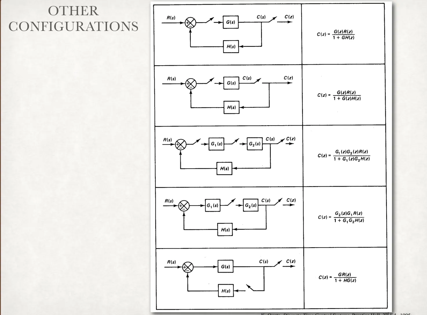
Table 4.1 Pulse Transfer Function of Five Typical Closed-Loop System Configurations From Figure 4.6, we see that

Y s( )= G s G( )⋅ _C*( )s E⋅ *( )s or Y s*( )= G s G*( )⋅ _C*( )s E⋅ *( )s Using the z-transform notation, we get

Y z( )= G z G z E z( )⋅ _C( )⋅ ( )

where G z( )= Z G s( ) . Since E z( ) = R z( )−Y z( ), we have

(19)

OUTLINE

(20)

CONTINUOUS-TIME PRECEDED BY ZOH

ME561 Lecture 5- 18

Continuous-time System Preceded by ZOH

[ ]

* ( ) _P ( ) _ZOH ( ) * * ( )

Y s = G s G⋅ s ⋅ U s G s e

ZOH s

Ts

( ) = 1− ⁻ Y z

U z( ) G s G_P _ZOH s G z ( ) = Z ( )⋅ ( ) = ( )

G z e

s G s G s

s e G s

s

G s

s z G s

s

Ts

P P Ts P P P

( ) ( ) ( ) ( ) ( ) ( )

=

L

−

NM O

QP

⁼

L

NM O

QP

⁻

L

NM O

QP

⁼

L

NM O

QP

⁻ ^⋅

L

NM O

QP

− − −

Z 1 Z Z Z ₁ Z

G z z G s

s

z z

G s s

P P

( ) ( ) ( ) ( )

= −

L

NM O

QP

⁼ ⁻

L

NM O

−

QP

1 ₁ 1

Z Z

Pure delay comes out directly

G_P(s) y(t)

Y(s) G_ZOH(s) u(k) or u*(t)

U(z) or U*(s) u(t)

Plant U(s) ZOH y(k) or y*(t)

Y(z) or Y*(z) G(z) or G*(s)

(21)

REVIEW OF ZOH

ME561 Lecture 5- 19

Review of ZOH

f t ( ) = f kT ( ) for kT ≤ < t ( k + 1 ) T

Unit Impulse Response

X s x t t t T

s s e e s

R R

sT

( ) = ( ) = ( ) − ( − )

= −

−

L L 1 L 1

1 1 1

G_ZOH(jω)

x*(kT) X*(jω) x_R(t)

X_R(jω)

Time 0

1

Time 0

1

T

G s e

ZOH s

sT

( ) = 1− ⁻

0 Time 1

T

“An integrator that is automatically reset to zero after one sampling period”

ME561 Lecture 5- 19

Review of ZOH

f t( ) = f kT( ) for kT ≤ <t (k +1)T

Unit Impulse Response

X s x t t t T

s s e e s

R R

sT

( ) = ( ) = ( ) − ( − )

= −

−

L L 1 L 1

1 1 1

G_ZOH(jω)

x*(kT) X*(jω) x_R(t)

X_R(jω)

Time 0

1 Time

0 1

T

G s e

ZOH s

sT

( ) = 1− ⁻

0 Time 1

T

“An integrator that is automatically reset to zero after one sampling period”

(22)

ME561 Lecture 5- 20

Ex4.2

( ) G s

( ) x t

*( ) y t

( ) X s

*( )

Y s zoh

*( )

x t ₁

( ) ( 1) G s = s s

+

Delays that are integer multiple of sample period can be taken out and replaced with the proper z^-1terms

[ ] [ ]

( )

2

1 1

1

( ) ( ) ( ) ( )

( 1) 1

( 1)

Ts

P ZOH

Ts

G z G s G s G s e

s e

s s

s s

−

− −

= = ⋅ ⋅

+

= ⋅

− +

Z Z = Z

Z

(

¹

)

2

1 1 (

z 1)

s s

= − ⋅

− Z +

( )

2

( ) 1 1 1 1

1 G z z 1

s s

s

∴ = − − ⋅ − +

Z +

(

¹

)

( 1 2

( 1 ) (1 )

1 ) 1 ( 1)( )

T T

T

T e z e Te

z z

z

z e e

T z

z z z

z

− − −

−

− + + −

−

= − − + = −

−

− −

−

(23)

ME561 Lecture 5- 21

Ex4.4

( ) G s

( ) x t

*( ) y t

( ) X s

*( )

Y s zoh

*( ) x t

G s K

P( ) = s a

+

1 ( ) 1

( ) (1 ) (1 )

( )

G sP k

G z z z

s s s a

− −

= − ⋅ = − ⋅

Z Z +

(

¹ ^z⁻¹

)

^K_a ¹_s _s ¹ _a ^z ⁻_{z a}¹ ^K ⁻¹ ¹_s _s ¹ _a

= − ⋅ − = ⋅ −

+ +

Z Z L

(

¹

)

¹ ¹

1 _at

t kT

e akT

z K z K

z a ⁻ z a e⁻

=

− −

= ⋅ Z − = ⋅ Z −

1 1

aT

z z e a z

z z

z K

−

= − −

−

(

¹ ^aT

)

aT

K e

a z e

−

= − −

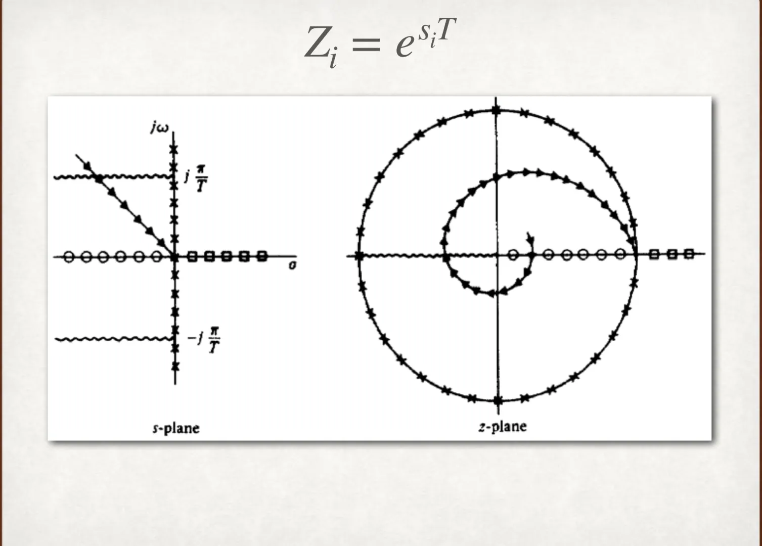
− C.T. pole: ^Note −a D.T. pole: e ^–aT ( recall z = e^sT )

(24)

AN IMAGINED APPLICATION

ME561 Lecture 5- 22

An Imagined Application

r(t) R(s) r(k)

R

^*

(s) C(z)

ZOH G(s)

U

^*

(s)

Y

^*

(s)

Y

^*

(s) u(k)

y(k)

e(k) E

^*

(s)

What techniques do we need for the analysis of this Control problem?

What techniques do we need for the analysis of

this control problem?

(25)

TABLE FOR SYSTEMS PRECEDED BY ZOH

ME561 Lecture 5- 23

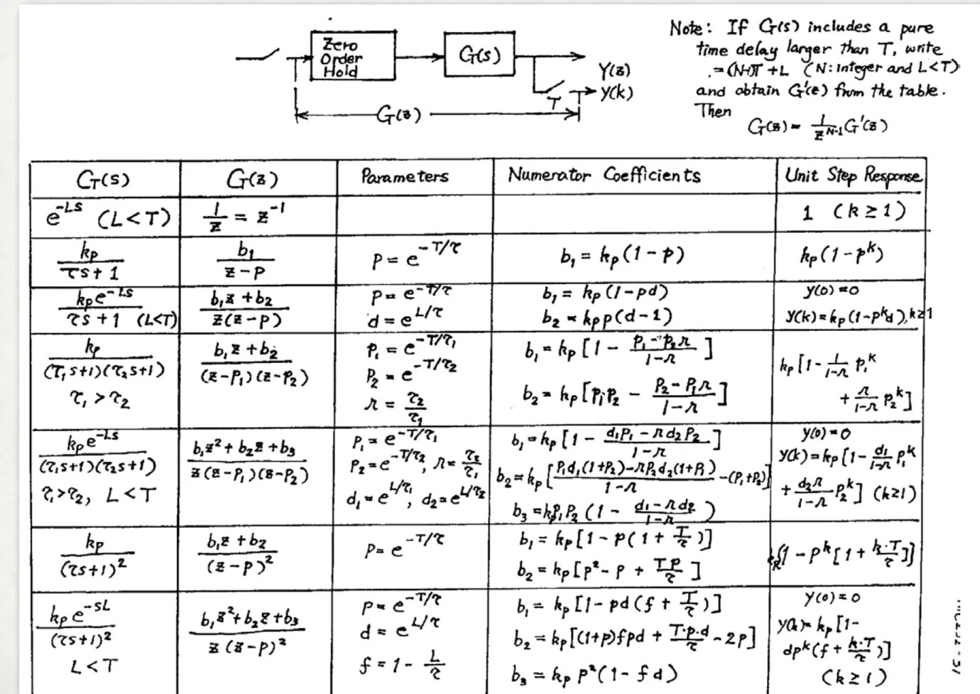
Table for Systems Preceded by ZOH

-- M. Tomizuka, ME232 Notes, UC Berkeley

(26)

ZOH EQUIVALENCE OF SYSTEM WITH TIME DELAY

ME561 Lecture 5- 24

ZOH Equivalence of System with Time Delay

G s_P

( ) =

e⁻^{T s}^D

⋅

G s

( )

TD = nT + TL

(

¹

)

1 ¹

( ) 1 ( )

1 ^L ^L

T T

n

s s

k n

t T

e G s z e G s

z z

s z s

− −

− − −

+

=

⋅ − ⋅

= − Z = Z L

(

¹

)

^{( )}

(

¹

)

^{( )}

( ) 1 1 ^L

T s p P

n s T

G s e G s

G z z Z z Z e

s s

− − − − ⋅

= − = −

(

¹

)

1

( ) 1 ( )

( ) 1 ^L^s ^L^s

p

n T

n

T G s z G s

G z z z e e

s z s

− −

+

⇒ = − ⋅ ⋅Z ⋅ = − ⋅Z ⋅

(27)

EX4.5 ZOH EQUIVALENT WITH TIME DELAY

ME561 Lecture 5- 25

Ex4.5 ZOH Equivalent with Time Delay

G s e

P s

s

( )

= .

+

−0 5

1

Find the equivalent ZOH transfer function with a sampling time of 0.2 sec.

Since T_D = 0.5 sec, we can select n = 2 and T_L = 0.1

Solution:

0.1

2 1 3

1 1 1 1

( ) ( 1) 1

s

z e z s

G z e

z s s z s s

− −

+

− −

= = −

+ +

Z Z

Use the following facts:

1

1 1

1 ^T

Z z

s z

Z z

s z e⁻

= −

+ = −

G

_p

(s) = e

^−0.5s

s + 1

(28)

ME561 Lecture 5- 26

Ex4.5 (cont.)

0.1 1 1

1 Z e s

s z

− =

−

0.1

0.1 0.1 0.1 0.2 0.1

1 1 0.2

1

1 ^k

s t T k

k

k e

Z e Z e Z e Z e

s z e

− − + − + ∞ − + −

= −

∞

= = = = =

+ −

( )

0.1

3 0.2 3

1 1 0.0952 0.0861

( ) 1 0.8187

z e z

G z z z z e z z

−

− +

= − =

− − −

0.1 1 2

1

1 1

1 0 1

s k

k

Z e z z z

s z

− ∞ − − −

=

= ⋅ = + + + =

∑

−

0.1

0.1 1 2

0

0.1 0.3

.2

1 0

1

s e

Z e z z

s e e z

e

− − − − − −

= + + + = −

+ −

(29)

OUTLINE

(30)

STATE SPACE REPRESENTATION

ME561 Lecture 6- 3

x(t) or x(k) n ¥ 1 vector State Vector u(t) or u(k) r ¥ 1 vector Input Vector

y(t) or y(k) m ¥ 1 vector Output Vector F or A n ¥ n matrix System Matrix

G or B n ¥ r matrix Input Matrix C(t) or C(k) m ¥ n matrix Output Matrix

D(t) or D(k) m ¥ r matrix Direct Transmission Matrix

State Space Representation

( ) ( ) ( )

t t t

= ⋅ + ⋅

x F x G u y C x D u

Continuous-Time

( 1) ( ) ( )

( ) ( ) ( )

k k k

+ = ⋅ + ⋅

= ⋅ + ⋅

x A x B u

y C x D u

Discrete-Time

(31)

STATE SPACE AND I/O

ME561 Lecture 6- 4

State Space and I/O

• Data needed to represent a LTI system:

( ) ( ) ( )

t t t

= ⋅ + ⋅

x F x G u y C x D u

( 1) ( ) ( )

( ) ( ) ( )

k k k

+ = ⋅ + ⋅

= ⋅ + ⋅

x A x B u

y C x D u

Continuous-Time Discrete-Time

F G C D

x x

y u

F G

C D u y

x ^{1 s} x

F G C D

A B C D

( )k x

( )k u

(k +1) x

( )k y

A B C D A B C D

( )k ( )k u

y

1 z x( )k (k +1)

x

Often referred to as system (A,B,C,D)

(32)

ZOH EQUIVALENT SYSTEM

ME561 Lecture 6- 5

ZOH Equivalent System

Given

the dynamics

and the selected sampling time T (for the sampling and ZOH),

can we figure out the equivalent discrete-time representation

x A x B u

y C x D u

( ) ( ) ( )

k k k

+ = ⋅ + ⋅

= ⋅ + ⋅

1

i.e., what is the relationship between (F,G) and (A,B)?

C and D remain unchanged.

F G C D

F G

C D u y

x 1 s x

( ) ( ) ( )

t t t

= ⋅ + ⋅

x F x G u y C x D u

A B

C D A B

C D u( )k ( )k

y

1 z x( )k (k +1)

x

ZOH ^u^{( )}^k

( )k

y F G

C D u

x 1 s x

y

ME561 Lecture 6- 5

ZOH Equivalent System

Given the dynamics

and the selected sampling time T (for the sampling and ZOH), can we figure out the equivalent discrete-time representation

x A x B u

y C x D u

( ) ( ) ( )

k k k

+ = ⋅ + ⋅

= ⋅ + ⋅

1

i.e., what is the relationship between (F,G) and (A,B)?

C and D remain unchanged.

F G C D

F G

C D u y

x 1 s x

( ) ( ) ( )

t t t

= ⋅ + ⋅

x F x G u y C x D u

A B

C D A B

C D u( )k ( )k

y

1 z x( )k (k +1)

x

ZOH ^u^{( )}^k

( )k

y F G

C D u

x 1 s x

y

DISCRETE-TIME SYSTEM REPRESENTATION