Suspicious Region Detection and Identification Based on Intra-/Inter-frame Analyses and Fuzzy Classifier for Breast Magnetic Resonance Imaging

Suspicious Region Detection and Identification Based on Intra-/Inter-frame Analyses and Fuzzy Classifier for Breast

Magnetic Resonance Imaging

Guo-Shiang Lin

, Sin-Kuo Daniel Chai

, Wei-Cheng Yeh

,Yi-Chang Lin

1*

First Name : Guo-Shiang Last Name : Lin

Affiliation : Associate Professor, Da-Yeh University

Phone : 886-4-8511888 ext. 2405 Fax : 886-4-5811350

Address : Dept. of Computer Science and Information Engineering, Da-Yeh University No.

168, University Rd., Dacun, Changhua County 51591, Taiwan E-mail: [email protected]

2

First Name : Sin-Kuo Last Name : Chai

Affiliation : Associate Professor, China Medical University Phone : 886-4-22053366 ext. 6312 Fax : 886-4- 22031108

Address : Dept. of Health Services Administration, China Medical University, Taiwan E-mail: [email protected]

3

First Name : Wei-Cheng Last Name : Yeh

Affiliation : Chief of Medical Imaging depart., Nantou Hospital Phone : 886-49-2231150

Address : Medical Imaging dept., Nantou Hospital, dept. of Health, Executive Yuan, Taiwan

E-mail: [email protected]

1

First Name : Yi-Chang Last Name : Lin

Affiliation : Master student, Da-Yeh University

Phone : 886-4-8511888 ext. 2405 Fax : 886-4-5811350

Address : Dept. of Computer Science and Information Engineering, Da-Yeh University No.

168, University Rd., Dacun, Changhua County 51591, Taiwan E-mail: [email protected]

Please send correspondence to Prof. Lin.

Email : [email protected]

ABSTRACT

Breast cancer is one of the leading causes of death from cancer in Taiwan. In this paper, we propose a feature-based scheme composed of preprocessing, feature extraction and a fuzzy classifier for suspicious region detection and identification. In the preprocessing stage, we first extract regions of interest and then coarsely determine suspicious regions via candidate screening. Some features are extracted based on intra-slice, texture, and inter-slice analysis techniques for suspicious region identification. Intra-slice analysis evaluates the intensity and size of suspicious regions. To find a precise region, we propose a region growing algorithm based on ellipse-based approximation. In texture analysis, some texture cues are extracted from spatial and wavelet domains and integrated as a combined texture feature by using a neural network. Inter-slice analysis is based on the continuity characteristic and consistency of a suspicious region’s size; the objective is to verify the static behavior of suspicious regions. Several MRI cases are utilized to evaluate the performance of the proposed scheme.

Experimental results demonstrate that our scheme can not only extract regions of interest but also identify tumors well from magnetic resonance images.

Keywords: suspicious region detection, fuzzy classifier, magnetic resonance imaging, MRI

I. INTRODUCTION

In Taiwan the mortality rate from breast cancer has increased markedly over the past two decades, and it is now the fourth leading cause of death from cancer. According to statistics published by the Department of Health [2], the death rate from female breast cancer increased from 3.9% in 1985 to 16% in 2011. In fact, breast cancer for women is one common cancer in many countries. Rangayyan et al. [5] observed that detecting breast cancer at an early stage will greatly improve the therapy and reduce mortality. However, detecting breast cancer at an early stage is extremely challenging. Currently, breast cancer is usually detected by mammography, ultrasonography, or magnetic resonance imaging (MRI) [17]. Mammography is an imaging tool that is widely used for early detection of breast cancer, and various computer-aided mammography methods have been developed [3],[6]-[8]. Ultrasonography is also a popular method for breast cancer diagnosis, but it is limited to detecting cystic lesions and advanced breast cancer [6].

In contrast to ultrasound and mammography, which have limitations in early breast cancer detection, MRI has demonstrated its greater capability and higher sensitivity for the task [17],[19]. This increased capacity is especially true for young women and for those with dense breasts. Some researchers have addressed the issue of detecting tumor regions for MR imaging [18],[28],[29],[30]. For instance, a segmentation method [18] based on dynamic programming and edge detection technique was proposed to segment the abnormal mass in breast MRI. However, it is often tough to clearly determine edges of abnormal masses, especially, dense breasts. In addition, due to dynamic programming and edge detection technique, the computational complexity is overly high to process all of breast MRI images.

A computer-aided diagnosis (CAD) system [28] was developed to explore breast MRI data.

However, a radiologist is needed to find the suspicious regions manually in this system [28].

Meinel et al. [29] proposed a lesion classification method for breast MRI. In the existing

method [29], a region growing algorithm where seeds are determined by an interactive thresholding is used to find out ROIs (region of interest) and some features are measured for each ROI. After feature extraction, a neural network is used to achieve lesion classification.

Nie et al. [30] proposed a diagnostic method for breast MRI. In the method [30], lesion segmentation is first performed by image subtraction and initial square ROIs should be placed manually to indicate suspicious areas. After segmentation, morphology and texture features are then measured and used with a neural network to achieve lesion classification.

However, since motion may exist between images, the segmentation by using image subtraction may result in some misclassified regions.

Even though some existing methods [18],[28],[29],[30] can be used for breast MRI, detecting tumor regions precisely is still a difficult problem, especially when the background is composed of organs, soft tissues and noise. Moreover, it is a very time consuming task for a physician to manually goes through all the slices and search for suspicious regions.

Physicians may miss suspicious regions. Hence, there is a need for a computer-aided diagnostic system based on MR imaging to reduce physicians’ workload in screening suspicious regions for tumor detection. This need motivated us to develop a suspicious region detection and identification scheme to achieve tumor detection for MR imaging.

ROI extraction has been used in many applications [20],[21],[22]. Since the size of a

MRI sequence is large, a ROI extraction algorithm was developed to raise the efficiency of

the proposed system. Because of the nature of tumors, it is difficult to detect them accurately

by using single-domain features. Intuitively, multiple features extracted from different

domains should be more useful in detecting suspicious regions. In addition, fuzzy logic is a

powerful tool to deal with imprecise and noisy data in real-world applications [14],[15],[26],

[27]. The main advantages of fuzzy rule-based systems are: 1) low memory

storage, 2) high inference speed and 3) high flexibility in adjusting fuzzy

rules [14],[15]. This means that a fuzzy system can be easily adjusted and expressed to model real-world problems, and it has better tolerance of imprecision. Based on this rationale, we have developed an efficient scheme that integrates different kinds of features and a fuzzy classifier with domain knowledge to detect suspicious regions simultaneously.

The remainder of this paper is organized as follows. In Section II, we introduce the proposed suspicious region detection scheme and discuss the first procedure. Section III describes the feature extraction process of the proposed detection system. In Section IV, we propose a fuzzy classifier for integrating different kinds of features. In Section V, we present the experiment results to demonstrate the efficacy of the proposed scheme. Section VI contains some concluding remarks.

II. PREPROCESSING

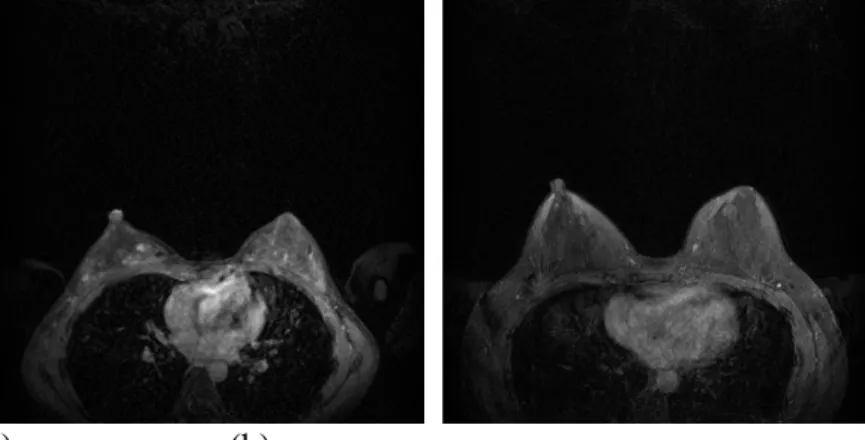
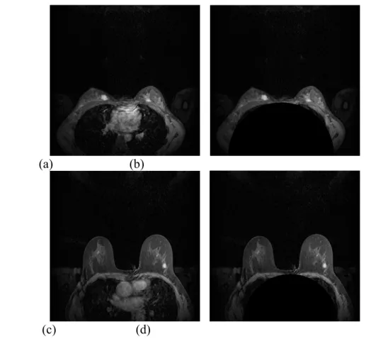
In [29] and [30], semi-automatic ROI detection was used to identify suspicious areas. To design a highly efficient mechanism for automatically detecting tumors in breast MR images, we should first analyze the characteristics of tumor regions. Figure 1 shows two MRI slices coming from different cases. As shown in the figure, each slice in a breast MRI is composed of organs, soft tissues, and noise. In addition, pixels with large values are located in the thoracic cavity as well as the breast. Although high intensity pixels are often associated with tumor regions, it is difficult to localize suspicious regions precisely by using only the information about pixel intensity. Therefore, we devise ROI extraction and candidate screening methods to detect suspicious candidate regions coarsely in a pre-processing stage.

Dissimilar to [29] and [30], we first perform automatic ROI extraction by removing the non-

interesting regions (non-ROIs) in the pre-processing stage. From the ROI region, we screen

some suspicious candidates and measure their characteristics as features. Then, using a fuzzy

classifier and the features, we can detect and localize suspicious regions. Figure 2 shows the

(a) (b)

Fig. 1. Examples of MRI slices for two cases: (a) Slice 53 of case 1; (b) Slice 74 of case 2

Fig. 2. Block diagram of our proposed suspicious detection and identification scheme

2.1 ROI extraction

In Fig. 1, the pixel values of some areas in the thoracic cavity are similar to those of

tumors; hence, detecting tumors correctly may be more difficult. According to physicians, it

is not possible for tumors to exist in the thoracic cavity. It is expected that removing some

parts of the thoracic cavity, especially organs and soft tissues, can reduce the difficulty of

detecting tumors. Figure 3 shows that a breast MRI slice is composed of a gray region (i.e.,

an ROI) and a semicircular region (i.e., a non-ROI). As shown in Figs. 1 and 3, the

semicircular region contains some organs and soft tissues. Therefore, we remove a part of the

thoracic cavity (i.e., non-ROI) to find the gray region (ROI) for further analysis.

Fig. 3. An illustration of ROI extraction in an MRI slice

As shown in Figs. 1 and 3, the semicircular region (i.e., non-ROI) can be localized according to two peak points (i.e., P

and P

) in the x direction. Therefore, to localize and remove the semicircular region, the steps of ROI extraction in each MR image are described as follows:

R1. Normalize an MRI slice via

   

 

 , , , 1,2,...,12 8 

max

, , ,

,  

t t y x I

t y x t I

y x

I

, (1)

where I  x , y , t  and I

 x , y , t  denote, respectively, the (x,y)-th original pixel value and the normalized pixel value in the t-th slice of an MRI sequence I; t is the slice number in the test MRI sequence; and ^max    is an operator used to find the maximum input value.

R2. Smooth the normalized image with a 33 average filter.

The smoothing operation reduces the impact of noise in the remainder of the procedure.

R3. Binarize the smoothed normalized image by thresholding; then label and select the

largest object.

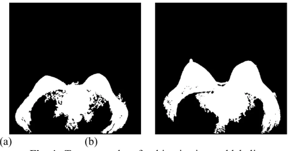
In the thresholding step, the average value of each smoothed normalized image is taken as the threshold. Based on Figs. 1 and 3, it is assumed that the largest object contains the breast. Figure 4 shows two examples after binarization and labeling. The figure shows that the largest object did contain the breast part after thresholding and labeling. However, the organs and soft tissues in the thoracic cavity are also included.

To resolve the problem the proposed scheme removes the semicircular region to achieve ROI extraction.

(a) (b)

Fig. 4. Two examples after binarization and labeling

R4. Find P

, P

, and P

for the largest object.

In this step, we first vertically project the largest object to find the leftmost and rightmost points, P

and P

, of the projected region on the horizontal axis, respectively. Based on P

and P

shown in Fig. 3, we can draw a vertical line L

passing through the point  0 ,  y

 y

 2  . Then, we can identify the intersection point P

of the vertical line L

and the chosen object’s contour. The y-coordinate of P

is



 / 2

3

y y

y   .

R5. Search peaks P

and P

on the left and right of P

, respectively, and find the point P

whose x-coordinate is the minimum between P

and P

.

To find the peaks P

and P

, we follow the contour of the chosen object from P

in both directions searching for the points with the largest x-coordinate on the left and right sides of P

. After obtaining P

and P

, the point P

can be found by searching for the point with the smallest x-coordinate between P

and P

along the contour of the chosen object.

R6. Draw the vertical line L

passing through the point P

, and derive the radius r is

 ^x

^{ k}

 , where x

is the x-coordinate of P

and k

is a constant. Then, the semicircular region whose radius is r and its center is at B

can be identified.

R7. Remove the semicircular region to obtain the ROI for further candidate screening.

2.2 Candidate screening

When searching for suspicious candidates, we consider two phenomena. First, we look for pixels with unusual pixel values because, according to [29] and physicians, the values of a tumor region are often higher than those of the surrounding regions. Second, a tumor region is small in the early stages, a useful cue that can be used to enhance the capability of detecting tumors at an early stage. Based on these two phenomena, we can coarsely screen suspicious candidate regions from ROI areas. The steps of suspicious candidate screening are as follows.

S1. Morphological opening

Because the intensity of tumor regions is usually high, morphological opening [1] is used here to separate the background from the foreground, which contains the candidate tumor regions. The foreground part can be obtained by

  t   t    t S 

R

I I 

I   , (2)

where  stands for the morphological opening operator [1], I   t denotes the t-th

original image, ^I

  ^t represents the resulting version after morphological opening and

subtraction, and S is the structure element in the morphological operator.

S2. Adaptive thresholding

It is expected that the range of pixel values as well as ^I

  ^t may not be similar in different MR images. Then adaptive thresholding can be used to select suspicious region candidates according to the following formula:

       

otherwise , max ,

, if 0 , 1

, I x y t T

T

t

t y x I

C C R

B



 

  , (3)

where ^I

 ^{x , y , t}  denotes the (x,y)-th pixel value in the t-th slice of the resulting version after morphological opening and subtraction; ^I

  ^t represents the result of adaptive thresholding in the t-th slice; T

is a predefined threshold; and ^T

  ^t denotes the threshold used to select several percentages of pixels with high values after morphological opening of the t-th slice. Based on Eq. (2), Eq. (3), and the definition of

  ^t

T

, the thresholding is adaptive.

S3. Connected component labeling

After adaptive thresholding, the chosen regions in the ROI are labeled. Actually, some labeled objects may only contain other tissues, such as blood vessels. To reduce the impact of such tissues on suspicious region detection, connected regions whose sizes satisfy a given constraint (e.g., smaller than T

(900)) are identified for the following shape refinement step.

2.3 Ellipse-based approximation with shape refinement

Although suspicious candidates can be obtained after morphological opening,

thresholding, and labeling, their regions may not be detected correctly. To analyze each

suspicious candidate accurately in the feature extraction phase, the shape of the candidate

must be refined. In addition, according to physicians, the shape of an early-stage tumor in an

MRI looks like an ellipse. Therefore, we adopt an ellipse-based approximation with shape refinement to represent each tumor candidate.

The ellipse-based approximation method was developed to find correct tumor regions and measure their properties, such as the center of mass (COM) and the best-fit ellipse [1]. To refine the shape of each suspicious candidate, we propose a region growing algorithm for each labeled candidate L

. For each labeled candidate L

, the steps of the algorithm are described as follows.

(G1) Compute the average intensity I

  t of L

and its COM as follows:

1 , 1

) , ( )

,

(

 









i

i l xy L

i c L

y l x i

c

y

y L L x

x , (4)

where ⁽ x

^, y

⁾ denotes the coordinate of COM of an object, L

denotes the i-th candidate in the l-th iteration, and L

represents the area of L

.

(G2) Measure D  x , y , t  and   x , y , t  as follows:

  _    











} 2 , 1 {

2 2

2 , 1 ,

i

f f

L

i

i

y y

x a x

t y

 x , (5)

 ^{x , y , t}   ^{x , y , t}   ^I  ^{x , y , t}  ^I   ^t 

D  



, (6)

where ^I

 ^x , ^y , ^t  is the pixel value of the neighboring pixel based on 8-

connectivity in the t-th slice; and  x ,

y

 (i=1,2) denotes the coordinates of the foci of an ellipse. The coordinates of the foci can be derived based the COM and the eccentricity of the ellipse. In [1], the semi-major axis a

in Eq. (5) is defined as

8 1

min 3 4 max 1

4 



 



 



 



 

I a

I

 , (7)

and

 











Li

y x

c

c

x x

y y I

) , (

2

min

( ) cos  ( ) sin  , (8)

 











Li

y x

c

c

x x

y y I

) , (

2

max

( ) sin  ( ) cos  , (9)

where sin    and cos    represent sine and cosine functions, respectively, and theta

 denotes the angle between the major axis and the x-axis (i.e., the horizontal axis).

According to Eqs. (6) and (7), the value of D  x , y , t  is small because a pixel is near the focal points of an ellipse and the pixel’s value is close to I   t

Li

. This means the neighboring pixel with small D  x , y , t  is similar to the pixels in the current candidate

(G3) Include neighboring pixels as their D  x , y , t  values are less than T (500).

(G4) Check whether the candidate overlaps the other candidates. If this situation exists,

merge the overlapping candidates, re-label all candidates, and return to Step (G1).

(G5) Check whether there are any neighboring pixels to be processed by calculating

 ^





D

i

L L

L . If ^L

is less than T (15), repeat Steps (G1) to Step (G4);

otherwise, stop.

III. FEATURE EXTRACTION

After pre-processing, we coarsely detect the suspicious regions in each slice; however, some

non-tumor regions may be misclassified as suspicious regions. For a suspicious detection and

identification scheme to be effective, the number misclassified regions should be reduced as

much as possible. It is expected that further analysis are necessary to confirm the status of

each suspicious candidate and thereby improve the performance of the proposed scheme.

According to physicians, there is no optimal representation of a tumor, so features extracted from different perspectives are useful for tumor detection. In addition, although the components of an MRI are complex, generally the characteristics of a tumor region are high intensity, small size, and complex texture, and there is continuity between the MRI slices.

Therefore, we extract these characteristics as features to reduce the number of possible errors.

As we need to analyze the continuity of each suspicious candidate, we apply 3D labeling to identify suspicious candidate objects before feature extraction. We elaborate on the types of analysis used for feature extraction in the following subsections. Note that the analyses are only applied to the selected candidate objects.

3.1 Intra-slice analysis

As the intensity value of a tumor region is a basic and effective characteristic for tumor detection [29], we measure the average intensity of a suspicious candidate as a feature. The average intensity of a suspicious candidate O

can be calculated as

 

   

 

 





 







i i i

i

N

t x,y O

N O i

O

O

I x y t

O I N

1

, 1 ,

1 , (10)

where I and

I

represent the normalized and average intensities of the i-th object O

respectively; and N

is the number of slices in which the i-th object O

occurs. It is

expected that the higher the value I

, the greater possibility that the object is a tumor.

However, as blood vessels may also be classified because they often exhibit high intensity, it is necessary to discover more features to improve the performance of tumor detection.

3.2 Inter-slice analysis A. Object continuity

In addition to intra-slice analysis, we perform inter-slice analysis to improve the

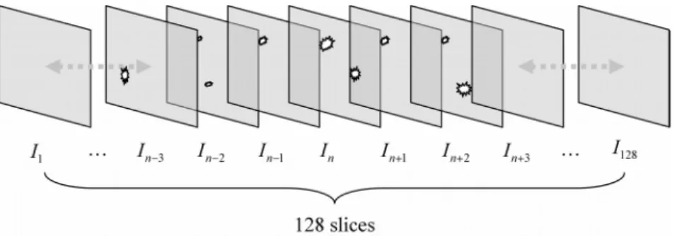
accuracy of suspicious region identification. Figure 5 illustrates the continuity of a tumor

with several slices. Generally, the position of a tumor region does not change significantly in a sequence of MRI slices. It is expected that recognized tumor regions in two adjacent slices should overlap and their COMs should be closed. Based on this assumption, a continuity test (CT) is performed on each candidate and its output is then exploited as a feature. To perform the continuity test, we measure the COM and the overlapped area between the recognized suspicious regions of two adjacent slices by checking whether

                 ^{ } _{ } ^ _ ^ _ 

otherwise

1 ,

min 1 1

1 ,

if 0

1  





 



 





 











 

 

i i

i i

i i

d i

O i

t T O t O

t O t t O

O t O T t

O t O t dist

C

,

(11)

where  is the logical AND operator;  is the intersection operator; min    is an operator for finding the minimum value of the input; O

  t and O

 t  1  denote the i-th suspicious regions in the t-th slice and the (t-1)-slice respectively; T and

T are thresholds; and

   

 ^{O t , O t  1}  ^  ^x   ^{t  x}  ^{t  1}  

^  ^y   ^{t  y}  ^{t  1}  

dist

is the Euclidean distance of the

COM between the t-th and (t-1) slices. Here, the values of T and

T are 5 and 0.8

respectively. For each suspicious candidate O

, a continuity test (CT) is performed on all MRI slices in a sequence.

Fig. 5. An illustration of continuity in inter-slice analysis

Actually, the size and pixel value of a tumor may change over several adjacent slices. It

is possible that a tumor may not be detected in one slice after per-processing, which means that the tumor may be divided into two small candidates. As a result, the continuity property of one of the small tumor candidates should be reduced and may make the proposed detector invalid. To solve the problem, we utilize the CT results in the two previous slices and the two subsequent slices to determine whether the CT result for the current slice is true or not. The rule is as follows: if the CT results in the two previous slices and the two subsequent slices are all true, the CT result of the current slice is also set as true, and the adjacent objects are grouped as a new object.

After adjusting the CT results, the continuity C

of a suspicious candidate can be expressed as

  





i i

N t

O

O

C t

C

1 1

,

. (12) In fact, C

measures the number of slices in which the candidate object is present.

According to physicians, if C

is large, the probability that the candidate object is a tumor is high.

B. Consistency of object size

As small blood vessels may occur in several adjacent images, they may be misclassified as a tumor. However, a blood vessel does not usually follow a straight line in several adjacent slices. We characterize this phenomenon as a feature in order to reduce the impact of blood vessels on suspicious region identification. The feature, denoted as C

,

analyzes the number of suspicious candidate objects that are larger than a threshold T

(9) in several adjacent images. It is defined as

   









i i

N t

A i

O

O

U O t T

C N

1

2 2

,

1 1 . (13)

where ^U   ^ denotes the unit step function ( U   x  1 for x  0 , and U   x  0 for x  0 ).

According to Eq. (13), the value of C

should be small if the suspicious candidate O

is a blood vessel; and the value should be high if the O

is located in a tumor.

3.3 Texture analysis

Texture has been generally utilized to detect and classify diseases as well as to segment suspicious regions in X-ray, ultrasound, MRI images [29],[30]. Similar to [29] and [30], texture information is also measured as features in the proposed scheme. The main reason is texture information in a tumor region differs from that in normal areas. Note that we only examine the pixels output during pre-processing. To extract texture information, we analyze each suspicious pixel and its neighboring pixels in a block. However, based on the extracted texture information, it is difficult to distinguish tumors from normal tissues when the block size is too small or large. In our experiments, we found that the best block size is 3232 pixels. Moreover, because texture cues can be measured in multiple domains, we compute the texture cues of each block in the spatial and wavelet domains. Therefore, in each MR image, a block of 3232 pixels centered at each pixel in the output of the pre-processing step is chosen as a candidate block for extracting texture features from multiple domains. Then, a neural network is used to fuse the texture cues into a single texture feature for tumor detection.

A. Spatial domain

In the spatial domain, we utilize three kinds of texture cues. First, we calculate the mean, standard deviation, and energy of the pixel values in each candidate block directly.

Second, as Law’s masks are popular for texture analysis, we also adopt them to extract

texture values. Following [11], we select two basic one-dimensional masks, R5 and W5, to

generate two two-dimensional masks, R5W5 and R5W5 respectively. Then, based on Law’s

mask, the TEM (texture energy measure) of each slice can be derived by the following

equations:

 

 









5 5

5

1

( , , ) , , R5W 5 ( , )

TEM

i j

t j i,y x t

y x I t

y

x , (14)

 

 









5 5

5

2

( , , ) , , W5R5 ( , )

TEM

i j

t j i,y x t

y x I t

y

x , (15)

 x,y , t  TEM  x,y , t  TEM  x,y , t 

TEM 



. (16) After computing the TEMs based on Eqs. (14)-(16), the mean and standard deviation of the TEMs for each suspicious candidate are calculated as texture cues by

 

 







i O

O yxt i

T

x,y t

f O

,1

1

1 TEM ,

, (17)

   

 





 



i O

O yxt

T i

T

tx,y f

f O

,1 2 1

2

TEM ,

1

1 . (18)

Finally, as the co-occurrence matrix, which characterizes the spatial distribution of intensity values in an image, is a popular and robust statistical tool for extracting texture information from images [3],[11],[12], we also extract some texture cues from a gray-level co-occurrence matrix. An element at location (i,j) of the matrix signifies the joint probability density of the occurrence of intensity values i and j in a specified orientation  and a specified distance d from each other. Thus, for different  and d values, different matrices are generated. The steps for extracting texture cues from a co-occurrence matrix are as follows.

(1) Quantize the pixel values in the candidate block into N

levels.

(2) Compute the co-occurrence matrix ^p

as

   

 

 









0 1 0

, , ,

, , ,

P P

N i

N j

d d d

j i M

j i j M

i p







, (19)

        

 

 

 



x N y

d

d

i j I x y i I x y j

M

1 1 ,

,_

, 

, , , , (20)

where 

 m , n  is the impulse function whose output is 1 only when m=0 and n=0. The two parameters, d and , represent, respectively, the distance and orientation between two pixels for generating the co-occurrence matrix. The relations between the (x,y)-th pixel and the ( x , ^y )-th pixel can be expressed as

 cos d x

x    and ^{y   y  d sin } . In this work, for each candidate block, we computed two matrices corresponding to two different directions ( ^ =0° and 90°), one distance (d=1 pixel), and N

=64.

(3) Calculate the following features from the obtained co-occurrence matrix:

(i) contrast: ^f

 ^{i j}  ^p

  ^{i j}

i N

j

T ^{P 1 P} _,

,

0 1 0

2

3

 









 , (21)

(ii) energy:  

 









0 1 0

2 ,

4 ^{P P}

,

N i

N j

d

T

p i j

f

, (22)

(iii) homegeneity:  

 







 



0 1 0

,

5

1

,

P P

N i

N j T d

j i

j i

f p

. (23)

B. Wavelet domain

The wavelet transform is a powerful tool that is used to analyze image content in many applications, such as image/video retrieval and image segmentation. After the l levels of 2D discrete wavelets decomposition [11],[31],[32],[35], there are 3l detail subbands (LL, LH, HL). In fact, these detail subbands contain texture information. Therefore, we analyze each candidate block and extract some texture cues from the wavelet domain. After 2D wavelet decomposition, the energies of three subbands (LL, LH, and HL) in each candidate block are computed as features. The steps for feature extraction in the wavelet domain are as follows.

(1) Transform the current block to obtain three subbands by using the Haar wavelet transform.

(2) Calculate the energy of the subbands (i.e., LH, HL, and HH) as texture features via

  



i j

b T

b

W i j

f

, , (24)

where ^W

 ^{i , j}  represents the wavelet coefficient in the b-th subband; and b denote the LH, HL, and HH bands respectively.

C. Texture cue fusion

As these texture cues are extracted from different domains and their ranges are different, we merge them to form a combined texture feature. Specifically, after extracting 14 texture cues, we utilize a supervised multi-layer feedforward neural network [39] to combine them. The neural network has three layers: input, hidden, and output. A linear transfer function is used for the input layer and logistic sigmoid transfer functions are used for the hidden and output layers. There are 14, 9, and 1 neurons in the input, hidden, and output layers, respectively.

In the training phase, we collect a large number of blocks classified by physicians into a training set. To train the neural network, the back-propagation and Levenberg-Marquardt algorithms are used [39]. To prevent over-training, we adopt the Q-fold cross-validation method [10]. That is, the training set is randomly divided into Q disjoint sets of equal size

Q

N

/ , where N

is the total number of samples. The (Q-1) sets selected arbitrarily from

the Q disjoint sets are exploited to train the neural network and the remaining set is used to

estimate the generalization error. The neural network is then trained Q times, each time with

a different set as the validation set. After training, because texture cues measured from spatial

and wavelet domains are the input of the neural network, the output of the neural network can

be exploited as a combined texture feature. Because a logistic sigmoid transfer function is

adopted in the output layer, the output range of the neural network is from zero to one. The

higher the output of the neural network is, the higher probability that a tumor exists will be.

Due to the main advantages of fuzzy rule-based systems mentioned in Section I, a fuzzy classification system was devised based on human knowledge and mathematical models. In terms of practicability, a trained fuzzy system can be exploited easily in real applications. Moreover, a fuzzy technique is often used to combine some features from different sources [15],[26],[27]. Therefore, based on the results of intra-slice, inter-slice, and texture analyses in the feature extraction phase, we can obtain four features for each suspicious candidate object to distinguish between tumors and non-tumors. For each suspicious candidate object, the four features are: (i) the average intensity f

of the pixel

values (i.e., I

); (ii) the object’s continuity f

(i.e., C

); (iii) the combined texture information f

(i.e., the output of the neural network); and (iv) the consistency f

of the

object’s size (i.e., C

). We integrate the above four features as the input for a fuzzy classifier to develop a tumor detector.

There are many types of fuzzifier, defuzzifier, and fuzzy inference engines [14] from which various systems can be built. Similar to the approaches in [14] and [15], we construct a fuzzy system comprised of a product inference engine, a singleton fuzzifier, and a center- average defuzzifier. The steps for constructing the above fuzzy system are detailed in [15].

Following [14] and [15], the output of the fuzzy system proposed this work is derived by



 

 

 



i f R

i f

N j

j f N i N j

j f N i j

v c

v

1 1

1 1





, (25)

where f

 (i=1, …,4) and v R  are the input and output of the fuzzy system, R respectively; v

is the center value of the output fuzzy set in the j-th rule (j=1,2,…, N

);

N

is the number of fuzzy rules; and  (i=1, …,

^N

) is the membership value of f

.

There is no standard procedure for devising the membership functions. As each feature

f

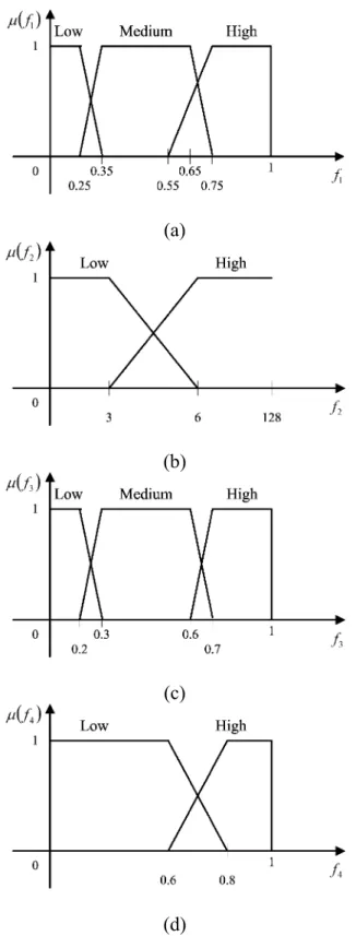
has a different impact on tumor detection, one way to obtain the corresponding member function is through heuristics. It is suggested that, to improve the performance of a fuzzy system, the fuzzy membership functions should be trained and adjusted by a large amount of training data. Based on this rationale, we conducted extensive experiments and propose four membership functions that correspond to the four features shown in Fig. 6, where “low”,

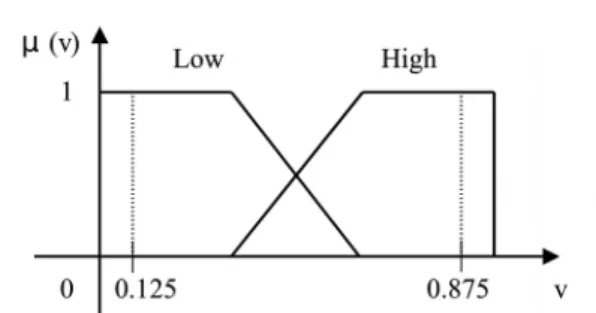
“medium”, and “high” are linguistic variables. The same design rationale applies to the membership functions of the output of the fuzzy system, as shown in Fig. 7.

The fuzzy rule base consists of a set of fuzzy if-then rules. Based on the four features, the above observation, and our experience, we define 36 rules in the fuzzy rule base. We do not list the rules because of space limitations. In Eq. (25), feature fusion is performed to process the membership values of all the features and obtain an output value. Then, based on the proposed membership functions of the input features and the output, a final decision can be made by using the following guidelines. The smaller the value of 

(v=L), the higher the probability that the current candidate is a healthy region. The larger value of 

(v=H), the greater the probability that the current candidate contains a tumor. To summarize, the decision rule is as follows:

Non-tumor, if _{ }  

v



H

max



= “Low”;

Tumor, if _{ }  

v



H

max



= “High”.

V. EXPERIMENTAL RESULTS 5.1 Dataset and parameter setting

To evaluate the performance of the proposed system for tumor detection, 18 true tumors in 8

T1-weighted MRI cases obtained from patients in Taiwan are used and their sizes are

different. In fact, there are three MRI sequences in each case and they correspond,

respectively, to before the contrast agent was injected, 2 minutes after the contrast agent was injected, and 7 minutes after the contrast agent was injected. As we aim at detecting tumors here, only the MRI sequence captured 7 minutes after injecting the contrast is tested in the proposed scheme. Each MRI sequence has 128 slices comprised of 512×512 pixels and contains more than one tumor region. The smallest and largest sizes of the small tumor in one slice are respectively 8 and 87 pixels; while the smallest and largest sizes of the large tumor are 107 and 805 pixels in one slice, respectively. Moreover, three physicians were involved in the creation of the gold standard for objective testing.

The proposed scheme is implemented by using Matlab. All of the parameters are

determined according to physicians’ opinions and our experience. For example, the size of

the structure element in the morphological opening is 25×25 pixels. Here, a training set for

neural network learning is comprised of 15,616 blocks and the size of each block is 32×32

pixels. To ensure that the neural network learning is representative, the blocks in the training

set are selected randomly from the MRI cases. To achieve supervised training, the training set

is divided into two classes: one class is comprised of 6,158 blocks and each block covers at

least a part of one tumor region; and the other composed of 9,458 does not contain tumor

regions. Here, the parameter Q in the Q-fold cross-validation method is set at 3.

(a)

(b)

(c)

(d)

Fig. 6. Membership functions of four input features: (a) the average intensity of the pixel

values, (b) the object’s continuity, (c) the combined texture information, (d) the

consistency of the object’s size

Fig. 7. Membership function of the output in the fuzzy classification system

5.2 Evaluation of ROI extraction

To evaluate ROI extraction, we employed subjective and objective tests. As shown in Fig. 4, the object containing the breast can be obtained after Step R3 in ROI extraction. After removing some parts of the thoracic cavity, Figure 8 shows two MR images and the results of ROI extraction. As shown in Fig. 8(b) and Fig. 8(d), it is appropriate to remove most of the thoracic cavity in both cases. A subjective test in which physicians viewed the results of ROI extraction was also performed. According to the physicians, ROI extraction is effective to find out the suspicious area where tumors may exist for all the test MRI slices.

In addition, the Hausdorff distance is often used as a measurement in image matching and image segmentation [11]. We adopt the Hausdorff distance as a metric to perform an objective test. Recall that the objective of removing the organs and soft tissues in the thoracic cavity for ROI extraction is to reduce the number of possible false alarms. As shown in Fig.

1, the organs and soft tissues are located near the middle of the thoracic cavity. Similar to the approach in [23], we use a weighted Hausdorff distance, where the weight in the middle of the thoracic cavity is high and the weights to the left and right of the thoracic cavity are low.

When the weighted Hausdorff distance is small, the boundary of the identified semicircular

region approaches that of the thoracic cavity. For 100 MRI slices, the weighted Hausdorff

distance is 5.46 pixels. According to Fig. 8 and the result of weighted Hausdorff distance, the

organs and soft tissues within the thoracic cavity in each slice can be appropriately eliminated

by using ROI extraction.

(a) (b)

(c) (d)

Fig. 8. (a)(c) Original MR images, and (b)(d) the results of removing the area of the thoracic cavity for ROI extraction

Figure 9 shows candidate regions (white areas) after pre-processing without/with ROI extraction. The original MR images coming from two cases are shown in the first column of Fig. 9 and the resulting images in the second and third columns show the candidate regions selected by pre-processing without/with the removal of non-interesting regions respectively.

There are two and one tumors in Fig. 9(a) and 9(d), respectively. As shown in Fig. 9(b) and

9(e), the candidate regions coarsely selected during pre-processing contain tumors. In

addition, though the sizes of tumors are different in Fig. 9(a) and 9(d), three tumors can be

found as candidates. However, there are misclassified regions, some of which result from the

thoracic cavity. Compared Fig. 9(f) with 9(c), some candidate regions resulting from the

thoracic cavity are removed due to ROI extraction. In addition, to evaluate the performance

of ROI extraction, the number of candidate regions for five test MRI cases are shown in

Table I. The statistics in the table show that the number of candidates can be reduced by ROI extraction. The result demonstrates that ROI extraction reduces the false alarms resulting from the thoracic cavity. Although most of the thoracic cavity can be removed, there are still some misclassified regions due to the existence of blood vessels, ducts, or noise. In fact, some pixel values in a blood vessel or duct region are sometimes high and the region’s shape is ellipse-like. As the characteristics (e.g., size and intensity) such regions satisfy thee conditions of size and intensity, they are deemed to be candidate regions.

(a) (b) (c)

(d) (e) (f)

Fig. 9. The evaluation of ROI extraction: (a)(d) original MRI images; (b)(e) resulting images without ROI extraction; (c)(f) resulting images with ROI extraction

Table I. The number of candidate regions without and with ROI extraction Without ROI extraction With ROI extraction Decrement

Case1 160 99 61

Case2 949 587 362

Case3 868 737 131

Case4 2598 1501 1097

Case5 11 11 0

Sum 4586 2935 1651

5.3 Overall performance analysis

Figure 10 shows the original MR images and the detection results of the proposed scheme. In Figures 10(a), 10(c), and 10(e), the true tumor regions are indicated with red lines drawn by physicians. The right column of Fig. 10 shows the detection result (white areas) of the proposed scheme. We observe that the proposed scheme can detect tumor regions correctly, as shown in Fig. 10(b), Fig. 10(d), and Fig. 10(f). Compared with Fig. 9, some candidate regions are removed by the following intra-, texture-, and inter-slice analyses.

Moreover, as shown in Fig. 10, these tumors among three cases can be detected though their sizes and locations are different. The results show that combining the intra-slice, texture, and inter-slice analyses improves the performance of the proposed scheme. The main reason is that after ROI selection, the texture information of these candidates is analyzed by using a neural network and their continuity is also evaluated. The different kinds of features combined by using a fuzzy classifier are used to identify tumors. However, there are still misclassified regions shown in Fig. 10 (d). Those regions result from the presence of blood vessels, ducts, or noise.

A receiver operating characteristic (ROC) graph is a common technique for visualizing and evaluating the performance of a classifier [10],[17]. Basically, a classifier’s performance is considered good if the trend of its ROC curve is toward the upper left-hand corner of the graph, i.e., the true positive (TP) rate is higher and the false positive (FP) rate is lower [33], [34],[36-38]. A higher TP rate means tumors can be correctly detected, whereas a lower FP rate which is equivalent to a higher true negative (TN) rate represents normal cases can be correctly identified. In this scenario, the area under the ROC curve should be close to 1.

Here we randomly select a part of MRI slices for training and the other for testing to

evaluate the proposed scheme 250 times. For example, we randomly choose three MRI cases

for training and the other for testing. In addition, we also change the threshold in the fuzzy classification to measure TPs and FPs for generating the ROC curve. Figure 11 shows that the ROC curve of our proposed fuzzy classifier approaches the upper left-hand corner of the graph, and the area under the curve is 0.91. Therefore, the results demonstrate that the proposed fuzzy classifier is effective in tumor detection for MR images.

(a) (b)

(c) (d)

(e) (f)

Fig. 10. The detection result for three cases: (a)(c)(e) original MR images (left) and (b)(d)(f)

detection results (right)

Here the sensitivity (also called recall), the positive predictive value (PPV) (also called precision) and specificity (i.e., TN) rates are also measured to evaluate the performance of the proposed scheme [17]. Sensitivity is a metric of completeness, whereas PPV and specificity are measures of accuracy for tumors and non-tumors, respectively. The higher the sensitivity, PPV and specificity rates, the better will be the performance of the proposed tumor detector.

For the test samples, the sensitivity rate of the proposed scheme is 100%, but the PPV and specificity rates are 79.4% and 82.1%, respectively. The results show that our proposed scheme can distinguish true tumors from normal regions effectively, but there are still some false alarms. Although the PPV rate is only 79.4%, physicians consider that the number of false alarms is within an acceptable range.

Fig. 11. The ROC curve of the proposed fuzzy classifier

VI. CONCLUSION

In this paper, we have proposed a feature-based scheme that comprises preprocessing, feature

extraction, and a fuzzy classifier for suspicious region detection and identification. In the

preprocessing phase, we first perform automatic ROI extraction to find out ROIs and then

coarsely determine suspicious candidate regions via candidate screening which is composed of a morphological operator, an adaptive thresholding and ellipse-based approximation. To identifysuspicious regions correctly for breast MR imaging, some features are extracted based on intra-slice, texture, and inter-slice analyses. In intra-slice analysis, the intensity and size information is utilized to find the candidates tumor regions. To localize a suspicious region accurately for further inspection, we propose a region growing algorithm based on the intensity and distance information. Some texture cues are extracted from different domains and merged to form a combined texture feature by using a supervised neural network during texture analysis. In inter-slice analysis, the continuity and size consistency of a suspicious region across slices is exploited to remove noise resulting from other tissues. After feature extraction, we use a fuzzy classifier to integrate the four kinds of features, which are then used to detect suspicious regions in the proposed scheme.

Several MRI cases are utilized to evaluate the performance of the proposed scheme.

The weighted Hausdorff distance is 5.46 pixels for 100 MRI slices. The result shows that the proposed ROI extraction can effectively remove some part of the thoracic cavity and reduce the number of false alarms substantially. In addition, the sensitivity and specificity rates of the proposed scheme are 100% and 82.1%, respectively. The results demonstrate that our scheme can be effective in detecting tumor regions from MR images.

In future, we may extract more features from MR images for suspicious region detection. In addition, we only analyze the MRI sequence captured 7 minutes after injecting the contrast. We may analyze other MRI sequences and then fuse those results for improving the performance of the proposed scheme.

REFERENCES

[1] A. K. Jain, Fundamentals Digital Image Processing, Prentice Hall, 1989.

[2] Health and Vital Statistics, http://www.doh.gov.tw/statistic/, Department of Health, Taiwan.

[3] S. C. Yang, C. M. Wang, Y. N. Chung, G. C. Hsu, S. K. Lee, P. C. Chung, and C. I.

Chang, “A Computer-Aided System for Mass Detection and Classification in Digitized Mammograms,” Biomedical Engineering Applications Basis and Communications 17 (2005) 215228.

[4] C. C. Lai, and C. Y. Chang, “A Hierarchical Evolutionary Algorithm for Automatic Medical Image Segmentation,” Expert Systems with Applications 38 (2007) 248259.

[5] R. M. Rangayyan, L. Shen, Y. Shen, J. E. Leo Desautels, H. Bryant, T. J. Terry, N.

Horeczko, and M. S. Rose, “Improvement of sensitivity of breast cancer diagnosis with adaptive neighborhood contrast enhancement of mammograms,” IEEE Trans.

Information Technology in Biomedicine 1 (1997) 161170.

[6] T. Arodz, M. Kurdziel, T. J. Popiela, E. O. D. Sevre, and D. A. Yuen, “Detection of clustered microcalcifications in small field digital mammography,” Computer Methods and Programs in Biomedicine 81 (2006) 5665.

[7] S. Joo, Y. Seok, W. K. Moon, and H. C. Kim, Computer-aided diagnosis of solid breast nodules: Use of an artificial neural network based on multiple sonographic features, IEEE Trans. Medical Imaging 23 (10) (2004) 12921300.

[8] I. El-Naqa, Y. Yang, M. N. Wernick, N. P. Galatsanos, and R. M. Nishikawa, A support vector machine approach for detection of microcalcifications, IEEE Trans. Medical Imaging 21 (2002) 15521563.

[9] M. L. Essink-Bot, A. J. Rijnsburger, S. van Dooren, H. J. De Koning, and C. Seynaeve, Women’s acceptance of MRI in breast cancer surveillance because of a familial or genetic predisposition, The Breast 15 (2006) 673676.

[10] R. O. Duda, P. E. Hart, and D. G. Stork, Pattern Classification, Wiley-Interscience, 2001.

[11] M. Sonka, V. Hlavac, and R. Boyle, Image processing, analysis, and machine Vision, Thomson, 2008.

[12] W. N. Lie, “An Efficient Threshold-Evaluation Algorithm for Image Segmentation Based on Spatial Graylevel Co-occurrences,” Signal Processing 33 (1993) 121126.

[13] T. Amin, M. Zeytinoglu, and L. Guan, “Application of laplacian mixture model to image and video retrieval,” IEEE Trans. Multimedia 9 (2007) 141621429.

[14] L. X. Wang, A course in fuzzy system and control, Prentice Hall PTR, 1997.

[15] D. H. K. Tsang, B. Bensaou, and S. T. C. Lam, “Fuzzy-based rate control for real-time MPEG video,” IEEE Trans. Fuzzy Systems 6 (1998) 504516.

[16] D. Cascio, F. Fauci, R. Magro, G. Raso, R.Bellotti, F. De Carlo, S. Tangaro, G. De Nunzio, M. Quarta, G. Forni, A. Lauria, M. E. Fantacci, A. Retico, G. L. Masala, P.

Oliva, S. Bagnasco, S. C. Cheran, and E. Lopez Torres, “Mammogram segmentation by contour searching and mass lesions classification with neural network,” IEEE Trans.

Nuclear Science 53 (2006) 28272833.

[17] A. P. Dhawan, Medical Image Analysis, John Wiley & Sons, 2003.

[18] J. Liu, W. Ma, and S. Y. Lee, “A segmentation method based on dynamic programming for breast mass in MRI images,” LNCS 4901 (2007) 307313.

[19] D. Vergnaghi, D. Trecate, and S. Manoukian, Breast Cancer, Springer Berlin Heidelberg, 2007.

[20] M. C. Chi, M. J. Chen, C. H. Yeh, and J. A. Jhu, “Region-of-Interest video coding based

on rate and distortion variations for H.263+,” Signal Process.-Image Commun. 23

(2008) 127-142.