Design of a Regressor-free Adaptive Impedance Controller for Flexible-joint Electrically-driven Robots
An-Chyau Huang
Department of Mechanical Engineering National Taiwan University of Science and Technology
Taipei, Taiwan [email protected]
Ming-Chih Chien
Mechanical and Systems Research Laboratories Industrial Technology Research Institute
Chutung, Taiwan [email protected] Abstract—To the best of our knowledge, this is the first paper
focus on the adaptive impedance control of robot manipulators with consideration of joint flexibility and actuator dynamics.
Controller design for this problem is difficult, because each joint of the robot have to be described by a 5th-order cascade differential equation. In this paper, a backstepping-like procedure incorporating the model reference adaptive control strategy is employed to construct the impedance controller. The function approximation technique (FAT) is applied to estimate time-varying uncertainties in the system dynamics. The proposed control law is free from the calculation of the tedious regressor matrix which is a significant simplification in implementation.
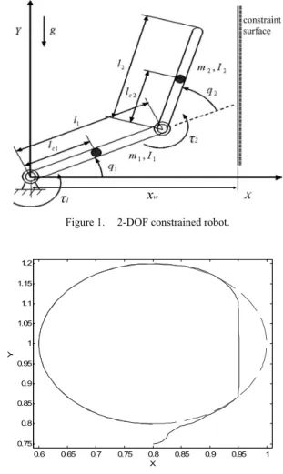
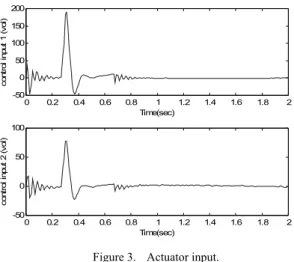
Closed-loop stability and boundedness of internal signals are proved by the Lyapunov-like analysis with consideration of the function approximation error. Computer simulation results are presented to demonstrate the usefulness of the proposed scheme.
Index Terms—Adaptive impedance control, Flexible joint electrically-driven robot, FAT
I. INTRODUCTION
Many industrial applications require robot manipulators to interact with the environment compliantly. Several control strategies have been suggested for this purpose. The well- known impedance control proposed by Hogan[1] is capable of giving a unified approach for controlling the robot in both the free space and constrained motion phase. Following the work of Hogan, several studies have been proposed[2-7]. However, most of these schemes ignore the effects coming from actuator dynamics and joint flexibility. As demonstrated in Good et al.[8] and Tarn et al.[9], in order to construct tracking controllers for high-velocity movement or highly varying loads, actuator dynamics constitutes an important part of the complete robot dynamics. Besides, the effects of joint flexibility may cause instability or resonance in the robot system, especially for a force controlled robot[10,11].
Therefore, the effects of actuator dynamics and joint flexibility should be taken into account in the control of a robot interacting compliantly with the environment if high performance is required. However, under these conditions, the cascade structure in the robot dynamics increases the complexity of the system model greatly, and a 5th order differential equation should be employed for describing a
This work was supported in part by the National Science Council of Taiwan, R.O.C., under Grant NSC97-2221-E-011-095.
single link. Hence, the controller design problem becomes extremely difficult.
Some controllers for constrained robots with consideration of joint flexibility and actuator dynamics were presented in Krishnan[12,13]. However, these strategies are only valid for the case when exact knowledge of the robot dynamics is available. Several works can be found for constrained robots with consideration of model uncertainties incorporating actuator dynamics[14-18] or joint flexibility[19-23]. Chien and Huang[36] proposed a backstepping-like procedure incorporating the model reference adaptive control for robots with consideration of both actuator dynamics and joint flexibility for operating in the free space. To our best knowledge, no work has been reported for the adaptive control of rigid-link flexible-joint electrically-driven (RLFJED) robots operating in the compliant motion applications.
In this paper, we would like to propose a FAT[24-36] based adaptive impedance controller for RLFJED robots. The design follows a backstepping-like procedure with the support of the model reference adaptive control to overcome the complex cascade structure in the robot dynamics, and the controller incorporates the impedance strategy to give a unified approach for controlling the robot in both the free space and constrained motion phase. The controller does not need to calculate the regressor matrix[37,38] which is required in the conventional robot adaptive design. The FAT is employed to deal with the time-varying uncertainties, which plays an important role in the construction of the update laws. The close loop stability and boundedness of internal signals are proved by using the Lyapunov-like technique with consideration of the approximation error. Simulation results are presented to demonstrate the usefulness of the proposed scheme.
II. MAIN RESULTS
The dynamics of a RLFJED robot interacting with the environment can be described by
ext T aF J q θ K q g q q q C q q
D( )&&+ ( ,&)&+ ( )= ( − )− (1a) Hi
q θ K θ B θ
J&&+ &+ ( − )= (1b)
u θ i, R i
L&+ ( &)= (1c)
where q∈ℜn is the vector of link angles, θ∈ℜnis the vector of actuator angles, i∈ℜn is the motor armature current vector,
ℜn
u∈ is the vector of control input voltage, D(q) is the
n× inertia matrix, n C(q,q& )q& is an n-vector of centrifugal and Coriolis forces, and g(q) is the gravity vector.
n a(q)∈ℜn×
J is the Jacobian matrix, which is assumed to be nonsingular in its working space. Fext∈ℜn is the external force exerted by the end-effector on the environment, and it is assumed to be precisely measurable by a wrist force sensor. J, B and K are n× constant diagonal matrices of the actuator n inertia, damping and joint stiffness, respectively. H∈ℜn×n is an invertible constant diagonal matrix characterizing the electro-mechanical conversion between the armature current and torque, L∈ℜn×n is a constant diagonal matrix of the electrical inductance, and R( θi,&)∈ℜn×n represents the effect of the electrical resistance and the motor back-emf.
The mapping from the control input u in (1c) to the link trajectory q in (1a) is in a special cascade form. A backstepping-like procedure is employed to facilitate the construction of the control strategy. The procedure starts from designing a desired trajectory for the transmission torque τd so that equation (1a) behaves like a given target impedance as defined in the traditional impedance control if
) (θ-q K
τt = [39,40] in (1a) converges to τtd, a desired τt. Then, a desired armature current id is designed such that (1b) can give proper performance. Finally, the control input is constructed in (1c) to ensure convergence of i to id. In this design, we would like to consider the case when the precise forms of D, C, g, L and R are not available and an adaptive impedance controller is to be designed without using the regressor matrix. Since the uncertainties are time-varying, traditional adaptive schemes do not apply. A FAT-based strategy is thus proposed to update the time-varying uncertainties so that an adaptive controller is realizable.
Define Jt = JK−1, Bt = BK−1 and q(q&,q&&)=Jq&&+Bq&
then (1a) and (1b) can be represented as
T ext a
t J F
τ q g q q q C q q
D( )&&+ ( ,&)&+ ( )= − (2) )
, ( qq q Hi τ τ B τ
Jt&&t+ t&t + t = − & && (3) It is often more convenient to describe the dynamics of the robot in the Cartesian space when interacting with the environment. Let x∈ℜn be the position vector of the end- effector in the Cartesian space and we may rewrite (2) as
Dx(x)x&&+Cx(x,x&)x&+gx(x)=Ja−Tτt−Fext (4) where
) ( )
(
] ) ( ) , ( [ ) , (
) ( )
(
1 1 1
q g J x g
J J J q D q q C J x x C
J q D J x D
aT x
a a T a
a x
T a a x
−
−
−
−
−
−
=
−
=
=
&
&
& (5)
In the traditional impedance control, all system parameters are given and a controller is designed so that the closed-loop system behaves like the target impedance
ext d
i d i d
i x x B x x K x x F
M (&&− && )+ (&−& )+ ( − )=− (6) where xd ∈ℜn is the desired trajectory of the end-effector in the Cartesian space, and Mi∈ℜn×n, Bi∈ℜn×n and
n i∈ℜn×
K are diagonal matrices representing the desired apparent inertia, damping, and stiffness, respectively. (6) implies that, in the free space tracking phase, i.e. Fext=0, the system trajectory converges to the desired trajectory asymptotically. On the other hand, in the constrained motion phase, it represents a stable 2nd-order LTI system driven by the external force. Conceptually, we may regard the impedance controller as a model reference controller. The target impedance plays the role of the reference model and the impedance controller drives the robot to follow the dynamics of the reference model in both the free space tracking and constrained motion phases. Since some of the system parameters are assumed to be unavailable in this paper, the traditional impedance controller is not feasible. Instead of (6), let us consider a new target impedance
ext d
i i d i i d i
i x x B x x K x x F
M (&& − && )+ (& −& )+ ( − )=− (7) where xi∈ℜn is the state vector of the target impedance (7).
If an adaptive impedance controller can be designed such that xi
x→ asymptotically, then the new target impedance (7) converges to (6) as desired.
Define signal vectors s= &e+Λe and v=x&i −Λe where xi
x
e= − is the state error, and Λ=diag(λ1,λ2,...,λn) with
>0
λi for all i=1, … n. Rewrite (4) in the form
ext T t
a x x x x
xs C s g D v C v J τ F
D &+ + + &+ = − − (8)
A. Controller Design for Known Robot
Suppose Dx, Cx and gx are known, and we may design a proper control law such that τ follows the trajectory below
)
( x x x d ext
Ta
t J g D v C v K s F
τ = + &+ − + (9)
where Kd is a positive definite matrix. Substituting (9) into (8), the closed loop dynamics becomes Dxs&+Cxs+Kds=0. Define a Lyapunov-like function candidate V = 21sTDxs. Its time derivative along the trajectory of system dynamics can be computed as V&1 =−sTKds≤0. It is easy to prove that s is uniformly bounded and square integrable, and s& is also uniformly bounded. Hence, s→0 as t→∞, or we may say that e→0 as t→∞. To make the actual τt converge to the perfect τt in (9), let us consider the reference model
td r td r td r r r r r r
rτ B τ K τ J τ B τ K τ
J && + & + = && + & + (10) where τr∈ℜn is the state vector of the reference model and
td ∈ℜn
τ is the vector of desired states which is equivalent to the perfect τt in (9). Matrices Jr∈ℜn×n, Br∈ℜn×n and
n r∈ℜn×
K are selected such that τr→τtd exponentially.
Define τtd(τ&td,τ&&td)=Kr−1(Brτ&td +Jrτ&&td) to be a function of x&&, F&ext, and F&&ext. Here, we may rewrite (3) and (10) in the state space form as
q B Hi B x A
x&p = p p + p − p (11)
)
( td td
m m m
m A x B τ τ
x& = + + (12)
where xp=[τTt τ&Tt ]T∈ℜ2n and xm =[τTr τ&Tr]T∈ℜ2n are
augmented state vectors. n n
t t t
n
p n 2 2
1
1 ×
−
− × ⎥∈ℜ
⎦
⎢ ⎤
⎣
⎡
−
= −
B J J
I A 0
and n n
r r r r
n
m n 2 2
1
1 ×
−
− × ⎥∈ℜ
⎦
⎢ ⎤
⎣
⎡
−
= −
B J K J
I
A 0 are augmented
system matrices. n n
p t ×
−⎥∈ℜ
⎦
⎢ ⎤
⎣
=⎡ 1 2
J
B 0 and
n n r
m r ×
− ⎥∈ℜ
⎦
⎢ ⎤
⎣
=⎡ 1 2
K J
B 0 are augmented input gain matrices,
and the pair(Am,Bm) is controllable. Let τt =Cpxp and
m m
r C x
τ = be the output signal vectors for (11) and (12), respectively, where Cp =Cm=[In×n 0]∈ℜn×2n. Note that the pair (Am,Cm) is observable and the transfer function
m m
m sI A B
C ( − )−1 is strictly positive real. Since all system parameters are assumed to be available at the present stage, we may select a perfect current trajectory in the form[41]
)]
, (
1[Θx Φτ h τ q
H
i= − p + td + td (13)
where Θ∈ℜn 2× n and Φ∈ℜn×n satisfy Ap+BpΘ=Am and BpΦ=Bm, respectively, and h(τtd,q)=Φτtd +q which is a function of q&& , θ&& , F&ext, and F&&ext. Substituting (13) into (11) and after some rearrangements, we may have the system dynamics
) ( td td
m p m
p A x B τ τ
x& = + + (14)
Defineem =xp −xmand we may have the error dynamics from (12) and (14)
m m
m A e
e& = (15)
Let eτ =τt−τr be the output vector of (15), and it can be rewritten as
m me C
eτ = (16)
Since Am is stable, (15) implies em →0 as t→∞. This further gives eτ →0 as t→∞. To ensure that the actual current i is able to converge to the perfect i in (13), let us select the control input in (1c) as
i c
d Ri,θ K e
i L
u= & + ( &)− (17)
where ei =i−id is the current error, id ∈ℜn is the desired current which is equivalent to the perfect current trajectory i in (13), and Kc∈ℜn×n is a positive definite matrix. Substituting (17) into (1c), the closed loop dynamics becomes
. 0 e K e
L&i+ c i = With this dynamics, it is easy to prove that id
i→ as t→∞ with proper selection of Kc.
B. Controller Design for Uncertain Robot
Suppose Dx, Cx, gx, L and R( θi,&) are not available, and q&& , θ&&, F&ext, and F&&ext are not easy to measure, we would like to design a desired transmission torque τtd so that a proper controller u can be constructed to have τt →τtd. Instead of (9), let us design a new desired transmission torque as
ˆ ) ˆ ˆ
( x x x d ext
Ta
td J g D v C v K s F
τ = + &+ − + (18)
where ˆ ,
Dx Cˆx and gˆx are estimates of Dx, Cx and gx, respectively. Substituting (18) into (8), we may have the closed loop dynamics
ˆ ) ( ˆ ) ( ˆ ) (
) (
x x x x x
x
td T t
a d x x
g g v C C v D D
τ τ J s K s C s D
−
−
−
−
−
−
−
= +
+ −
&
&
(19) If a proper controller and update laws for ˆ ,
Dx Cˆx and gˆx can be designed, we may have τt→τtd, ˆ ,
x
x D
D → ˆ ,
x
x C
C → and gˆx →gx so that (18) can give desired performance. Let us have a modify version of the desired current id as
ˆ)
1(Θx Φτ h
H
id = − p + td + (20)
where hˆ is an estimate of h. Hence, the system dynamics can be derived as
ˆ) ( )
(i i B h h
H B τ B x A
x&p = m&p+ m td+ p − d − p − (21) Together with (12), we may have the error dynamics
ˆ)]
(
[He h h
B e A
e&m= m m+ p i− − (22)
m me C
eτ = (23)
Instead of (17), let us select the control input in (1c) as
i ce K f
u= ˆ− (24)
where fˆ is an estimate of f(i&d,i,θ&)=Li&d +R(i,θ&).
Substituting (24) into (1c), we may have the system dynamics ˆ)
(f f e
K e
L&i+ c i =− − (25)
If an appropriate update law for fˆ can be selected, we may have i→id. Since Dx, Cx, gx, h, L and f are functions of time, traditional adaptive controllers are not directly applicable. To design the update laws, let us apply the function approximation representation[24-36]
f f f h
h h g
g g
C C C D
D D
ε Z W f ε Z W h ε Z W g
ε Z W C ε Z W D
+
= +
= +
=
+
= +
=
T T
x T
x T x T
x x x
x x x x
x x
,
,
,
, (26a)
whereW(.) are weighting matrices,Z(.) are matrices of basis functions, and ε(⋅) are approximation error matrices. The number β represents the number of basis functions used. (⋅) Using the same set of basis functions, the corresponding estimates can also be represented as
f f h
h
g g C
C D
D
Z W f Z W h
Z W g Z W C Z W D
T T
x T x T
x Tx x x x x x
ˆ ˆ ˆ ,
ˆ
ˆ , ˆ ˆ ,
ˆ ˆ ,
ˆ
=
=
=
=
= (26b)
Define ~() () ˆ()
⋅
⋅
⋅ =W −W
W , then equation (19), (22) and (25) becomes