3-1 Fourier transform infrared spectrometer

Chapter 3

Experimental optical techniques

Optical spectroscopy has been proved to be the effective tool for probing the internal excitations of materials.^[43] At far-infrared frequencies, insulators such as antiferromagnetic insulator oxides CaCu3Ti4O12, CaMnO3, and Sr2YRuO6 do not have free electrons to interact with light. Phonons play an important role when insulating crystals interact with light. On the other hand, at higher frequencies, the energy of incoming light becomes comparable to the interband transition energy, an occupied electron in the valence band could be excited to unoccupied state in the conduction band. The optical transitions are measured by the magnitude of the momentum matrix elements coupling with the valence band state i and the conduction band state f ( i p f ²). The dependence results from Fermi golden rule.^[44] The optical spectra at high frequencies provide information of the electronic structure of materials.

3-1 Fourier transform infrared spectrometer

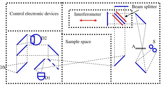
A vacuum Fourier transform infrared spectrometer (Bruker IFS 66v/s) was used for the the far-infrared (FIR: 50 ~ 650 cm^-1) and middle infrared (MIR: 370 ~ 6000 cm^-1) measurements. In order to obtain high-solution optical spectra, FTIR spectrometer was constructed based on the Michelson interferometer.^[45] Figure 3 – 1 illustrates the experimental setup of the FTIR spectrometer. It is composed of two light sources, beam splitters, and detectors, which can be changed under the computer control. In FIR region, a mercury light setting, a multilayer T222 beamsplitter, and a Si bolometer were used; in MIR region, a golbar light, a KBr T301 beamsplitter, and a deuterated

triglycine sulfate (DTGS D301) were used. We use the near-normal incidence (the angle between incident ray and reflected ray is less than 11°) configuration. In order to collect the correct reflectance spectra data, we used gold mirror as a reference in our FIR and MIR measurements due to its 100% reflectance in FIR and MIR regions.The correct reflectance spectra R_exp are obtained by the following equation,

sample

.

Au Au

measured

textbook sample measured

R R R

= R ×

3-2 Grating monochrometer

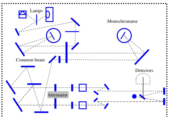
PerkinElmer Lambda 900 is a high-energy system that enables spectral recording from 3850 to 55000 cm^-1. Figure 3 – 2 presents the experimental setup of the Lambda 900 spectrometer. It contains double-beam and double-monochromator (grating-type) spectrophotometer with holographic gratings, large collimating mirrors and computer-controlled synchronized slit mechanisms. The grating-type monochromator is composed of an entrance slit, a grating, and an exit slit, which is suitable for medium or high resolution in comparison with a prism-type monochromator.^[46]

Double-monochromator has two principle advantages: including (a) it can decrease the value of stray radiation to 0.00008﹪in comparison with 0.01 of single monochromator (stray radiation may originate from the specimen holder, or from parts of the instruments.), and (b) it can provide more accurate wave length. After passing through the double-monochromator, beam light certainly decrease its intensity. So that, a chopper was used to change the path of light, which is in order to reduce uncertainties that are caused by the lower intensity of light. In near-infrared (NIR) and visible (VIS) region, the tungsten lamp and photoconducting detector were used. In ultraviolet (UV)

region, the deuterium lamp and photomultiplier tube were used. In order to collect the correct reflectance spectra data, we used Al mirrors as a reference in our measurements.

A continuous flow helium cryostat was used for the low-temperature measurements. Figure 3 – 3 illustrates the experimental setup of the cooling system.

The experimental setup provides the measurements at the temperature range from 10 K to 340 K.

3-3 Optical theory

Our emperimental data were collected as reflectance spectra data, so we first introduce the reflection of light at a plane surface between two media of different dielectric properties.^[45,47] The incidence, reflected, and transmittance light in plane form can be written as

( )

0

( )

0

( )

0

, , .

i

r

t

i k r t

i i

i k r t

r r

i k r t

t t

E E e E E e E E e

ω ω ω

−

−

−

=

=

=

i i i

(3-3-1)

We consider the electric field perpendicular to the plane of incidence (TE mode).

The dynamic properties are contained in the boundary conditions–normal components of D and B are continuous and tangential components of E and H are continuous. Within the general consideration of the nonmagnetic materials, the representation of the reflectance and transmittance coefficients as the Fresnel coefficient can be written as

0

0

0

0

cos cos

cos cos , 2 cos cos cos ,

r i i t t

TE

i TE i i t t

t i i

TE

i TE i i t t

E n n

E n n

E n

E n n

θ θ

γ θ θ

θ

θ θ

⎛ ⎞ −

≡ ⎜ ⎝ ⎟ ⎠ = +

⎛ ⎞

Γ ≡ ⎜ ⎝ ⎟ ⎠ = +

(3-3-2)

where γ_TE is the reflectance coefficient, and Γ is the transmittance coefficient. _TE When the electric field is parallel to the plane of incidence (TM mode), the reflectance and transmittance coefficients can also derived at the same way as

0

0

0

0

cos cos

cos cos , 2 cos cos cos .

r t i i t

TM

i TM i t t i

t i i

TM

i TM i t t i

E n n

E n n

E n

E n n

θ θ

γ θ θ

θ

θ θ

⎛ ⎞ −

≡ ⎜ ⎝ ⎟ ⎠ = +

⎛ ⎞

Γ ≡ ⎜ ⎝ ⎟ ⎠ = +

(3-3-3)

For the near-normal light configuration (θi ~ 0°), both equations (3-3-2) and (3-3-3) reduce to

( )

( )

( )

, 2 .

i t

TE TM

i t

i TE TM

i t

n n n n n n n

γ = − ⁻

+

Γ =

+

(3-3-4)

In our measurements, the intensity we measured is the magnitude of the electric field, so that the reflectance data is the square of the reflectance coefficient, which can be written as,

2 2

2

2

,

r i t

r

i i i t

E n n

R I

I E n n

γ ⁻

= = = =

+

Now, we consider our measurements that ni is the refractive index of the air and

supposed to be 1. The n_t is the refractive index of our sample, so n_t is a complex function (n). Therefore, the reflectance can newly be written as

2 2 2

1 1 1

1 ,

1 1

n n ik

R n n ik

ε ε

− − − −

= = =

+ + + +

where n and k are the refractive index and the extinction coefficient. The other complex optical parameters ( ( )f ω = f′( )ω +if′′( )ω ) such as σ , n, and ε can be obtained by carrying out a Kramer-Kronig analysis of our reflectance data. We now discuss the Kramer-Kronig analysis, and the Kramer-Kronig relations can be written as^[45]

2 2

0

2 2

0

1 2 ( )

( ) ,

( )

1 2 ( )

( ) ,

( )

f f d

f f d

ω ω

ω ρ ω

π ω ω

ω ω

ω ρ ω

π ω ω

∞

∞

′ ′′ ′

′ = ′

′ −

′ ′ ′

′′ = − ′

′ −

∫

∫

where ρ indicates the Cauchy principal value.

The complex reflectance coefficient associated with the reflectance data we collected can be rewritten as

( )

( ) ( ) ( ), 1 ( ) ( )

( ) ( ) ,

1 ( ) ( ) ln ( ) ln ( ) ( ).

i

i n ik

R e n ik

R i

φ ω

γ ω γ ω γ ω

ω ω

γ ω ω

ω ω

γ ω ω φ ω

′ ′′

≡ +

− −

= =

+ +

= +

(3-3-8)

To combine the equations (3-3-7) and (3-3-8), the phase part of the reflectance coefficient can be obtained as

2 2 0

ln ( ) ln ( )

( ) 2 .

( )

R R

ω ω d

φ ω ω ρ ω

π ω ω

∞

′ − ′

= ∫ − ′

After putting equation (3-3-9) into (3-3-8), we can obtain the n and k in terms of ( )

R ω and ( )φ ω as

1 ( )

( ) .

1 ( ) 2 ( ) cos ( ) 2 ( ) sin ( )

( ) .

1 ( ) 2 ( ) cos ( ) n R

R R

k R

R R

ω ω

ω ω φ ω

ω φ ω

ω ω ω φ ω

= −

+ −

= + −

(3-3-10)

All the optical parameters are related to each other, so we can calculate all optical parameters by means of n( )ω and k( )ω for example the εand n can be obtained by putting equation (3-3-10) into (3-3-6). The real part optical conductivity spectra data σ ω₁( ) were also obtained by applying KK transformation to the reflectance data. The usual requirement of the KK integrals is up to infinity, so that the extension of the reflectance at low-frequency and high-frequency ends is important. At low frequencies, the extension was done by keeping the reflectance constant to dc, as appropriate for insulators. The high-frequency extrapolations were extended by using the standard power law R ~ ω^-s (s ~ 1–2).

Fig. 3 – 1. Experimental setup of the fourier transform infrared spectrometer (BRUKER IFS 66v/s). (S: light sources, A: aperture, and D: detectors.)^[45]

Control electronic devices Interferometer

Sample space

Beam splitter

S A

D1 D2

DX

Fig. 3 – 2. Experimental setup of the UV/VIS/NIR spectrometer (Perkin Elmer Lambda 900).

Common beam

Monochromator

Attenuator

Detectors Lamps

Fig. 3 – 3. Experimental setup of cooling system.