應用於顫振辨識之特徵選擇與分類方法之研究

(1)

國立台灣大學工學院機械工程研究所碩士論文

Graduate Institute of Mechanical Engineering College of Engineering

National Taiwan University Master Thesis

應用於顫振辨識之特徵選擇與分類方法之研究 A study of feature selection and classification methods for

chatter identification models

陳宇軒 Yu-Hsuan Chen

指導教授:劉建豪博士 Advisor: Chien-Hao Liu, Ph.D.

中華民國 108 年 6 月 June, 2019

(2)

(3)

誌謝

首先要感謝指導教授劉建豪老師，在碩士班這兩年給我的指導與支持，並在研究上遇到困難時幫忙找資源協助我，讓我在實驗室這兩年學習到許多做研究的方法。也感謝施文彬老師，在我碩一時提供了許多研究方向的建議與指教，使我受益良多。口試委員蔡孟勳教授及蔡曜陽教授也提供了許多專業的見解，對這篇論文的研究提供了寶貴的意見與回饋，感謝你們的參與。

這篇研究可以順利完成，一部分要感謝泳辰學長的建議以及當初建立的研究方向。傑程與胤瑄平時提出的問題與想法也幫助我更仔細的思考研究上遇到的一些問題。感謝實驗室的夥伴們，星宇，善謙，建章，尚軒，家倫，炫奇，健宏，柏文，碩志，晉祥，永珊，均鴻，謝謝你們的幫忙與陪伴。也感謝家人一路上的支持，讓我可以順利完成這個學位。

(4)

中文摘要

維持高產率對於銑削加工的效率而言十分重要。顫振是加工時發生的一種自激式振動，在實務中限制了產率。過去的研究提出了許多顫振偵測的方法，利用各種訊號處理的方法如快速傅立葉轉換(FFT)，小波包轉換(WPT)，及希爾伯特 -黃轉換(HHT)。許多資料分類演算法也被應用於顫振偵測。雖然顫振偵測的領域已有許多文獻，我們仍不清楚何種方法可以達到較佳的正確率與偵測速率。

在本研究中，我們將測試多種訊號處理方法以及資料分類的演算法，使用的資料集中包含各種主軸轉速及切深。我們結合多種訊號處理方法及分類演算法，

開發了一個顫振辨識平台以建立分類模型並評估其性能。資料分類方法包含了固定的閾值，最近鄰居法(k-NN)，單純貝氏分類器，支持向量機(SVM)，局部密度因子(LOF)，以及類神經網路。以分類精準度而言，結果顯示最近鄰居法搭配小波包轉換及希爾伯特-黃轉換是最佳的方法，誤判率僅 2.2%。

關鍵字: 顫振，小波包轉換，希爾伯特-黃轉換，最近鄰居法，支持向量機

(5)

Abstract

Maintaining high production yield is important for efficiency in the milling process.

Chatter is a type of self-excited vibration that can occur during machining, and limits the production yield in practice. In the past, many chatter detection methods were proposed using different signal processing methods such as Fast Fourier transform (FFT), wavelet packet transform (WPT), and Hilbert-Huang transform (HHT). Several classification methods were also applied in chatter detection. Despite the large amount of researches regarding chatter detection, it is unclear which of these proposed methods are better in terms of accuracy and detection speed.

In this research, we test the signal processing methods and classification algorithms against the entire dataset, with a wide range of spindle speeds and depth of cuts. A chatter identification platform is developed to train models and evaluate their performance, using combinations of signal processing methods and classification algorithms. The classification methods include numerical threshold, k-nearest neighbors (K-NN), Naïve Bayes, support vector machine (SVM), local outlier factor (LOF), and artificial neural network. K-NN proves to be the optimal method when using WPT and HHT for signal processing, with an error rate of 2.2%.

Keywords: chatter, wavelet packet transform, Hilbert-Huang transform, k-nearest neighbor, support vector machine

(6)

List of figures

Fig. 1. Chatter leaving undesired marks on the surface of the workpiece [9] ... 13

Fig. 2. Illustration of how chatter develops due to abrupt change in chip thickness [2] 13 Fig. 3. An example of a stability lobe diagram [14] ... 14

Fig. 4. (a) Spectrum of the vibration signal after FFT, (b) Intrinsic mode functions (IMFs) obtained from Hilbert-Huang transform [40] ... 15

Fig. 5. Illustrations of LOF and SVM ... 16

Fig. 6. Power spectrum density (PSD) obtained by applying FFT on the sound signal during cutting. [56] ... 20

Fig. 7. Illustration of window and overlap ... 22

Fig. 8. Various families of mother wavelets, including (a) Haar, (b) Daubechies (db), and (c) biorthogonal (bior). [58] ... 23

Fig. 9. Wavelet transform produces lower frequency resolution at high frequencies .... 24

Fig. 10. Wavelet packet transform and its corresponding coefficient tree for each frequency bands [59] ... 25

Fig. 11. Illustration of the concept of autocorrelation coefficient ... 27

Fig. 12. IMFs of a cutting signal obtained using HHT ... 31

Fig. 13. Illustration of Hilbert transform on vibration signal [67] ... 31

Fig. 14. Hilbert spectrum of unstable (left) and stable (right) cutting signals calculated and visualized with MATLAB ... 32

Fig. 15. An example of visualized local outlier factors ... 36

Fig. 16. (a) Illustration of linear SVM for a linearly-separable dataset [78] (b) Non- linear SVM with RBF kernel [79] ... 37

Fig. 17 Architecture of model training platform for chatter identification ... 41

(9)

Fig. 18. Illustration of the computation of discrete convolution ... 44

Fig. 19. Illustration of the peak finding procedure and the calculation of prominence of a peak ... 46

Fig. 20. Illustration of stratified k-fold validation [47] ... 47

Fig. 21 Experiment setup when gathering the dataset ... 49

Fig. 22. Test costs of LOF for each of the three test datasets, and the average costs ... 50

Fig. 23. Test error rates of K-NN for each of the three test datasets, and the average error rates. ... 52

Fig. 24. Error rates when different classification methods are used with the same feature (FFT relative energy) ... 54

Fig. 25. FFT spectrum raised to exponent p for p = 0.5, 1, 2.75, and 8 ... 56

Fig. 26. Effect of exponent p on classification error rates ... 57

Fig. 27. FFT relative energy plots for (a) p = 0.5, (b) p = 1, (c) p = 2.75, and (d) p = 8 ... 58

Fig. 28. Comparison of error rates with different FFT related features ... 63

Fig. 29. Comparison of average error rates within each mother wavelets family ... 65

Fig. 30. Comparison of average error rates within each mother wavelets family ... 66

Fig. 31. Comparison of average error rates when different axes are used as feature in k- NN classifier ... 66

Fig. 32. Normalized relative energies 𝐸′𝑊𝑃𝑇(𝑦) and 𝐸′𝑊𝑃𝑇(𝑧) using WPT ... 68

Fig. 33. Autocorrelation coefficient for a stable cut ... 70

Fig. 34. Autocorrelation coefficient for an unstable cut ... 70

Fig. 35 Autocorrelation coefficient of (a) original acceleration signal, (b) velocity signal, and (c) displacement signal. ... 71

Fig. 36. Distribution of standardized phase differences 𝜀 for x-, y-, and z-axes. ... 72

(10)

Fig. 37. Phase differences 𝜀 of the entire dataset, in x-, y-, and z-directions. ... 74 Fig. 38. Distribution of the y- and z-axis relative energy after only HHT (top), and WPT+HHT (bottom) ... 78 Fig. 39. Comparison of average error rates when different axes are used as feature ... 79 Fig. 40. Probability distribution function (PDF) of the y-axis features used in this research, for both stable and unstable categories, including (a) 𝐸1, 𝐹𝐹𝑇, (b) 𝐸2, 𝐹𝐹𝑇, (c) 𝐸3, 𝐹𝐹𝑇, (d) 𝐸𝑊𝑃𝑇, (e) 𝜖 from autocorrelation coefficient, and (f) 𝐸𝐻𝐻𝑇 ... 81 Fig. 41. Comparison of error rates of all features ... 82 Fig. 42. Variation of error rates with respect to window size for (a) EFFT, 1, (b) WPT, (c) phase ε for autocorrelation coefficient, and (d) HHT ... 84 Fig. 43. Variation of detected time with respect to window size for (a) 𝐸𝐹𝐹𝑇, 1, (b) WPT, (c) phase 𝜀 for autocorrelation coefficient, and (d) HHT. ... 86 Fig. 44. Relative detected times for each different feature and window sizes for FFT (𝐸1, 𝐹𝐹𝑇), WPT, autocorrelation coefficient, and HHT (with WPT) ... 87

(11)

List of tables

Table 1. Major libraries used to implement the platform ... 42 Table 2. Performance test on numpy.fft.rfft() ... 43 Table 3. Classification error rates using FFT (𝐸1, 𝐹𝐹𝑇) and different unstable data point ratio in LOF ... 51 Table 4. Classification error rates using k-NN and different weights ... 53 Table 5. Classification error rates using FFT (𝐸1, 𝐹𝐹𝑇) and different filter bandwidths ... 59 Table 6. Classification error rates using FFT (𝐸1, 𝐹𝐹𝑇) and different window sizes .... 60 Table 7. Error rates using 𝐸1, 𝐹𝐹𝑇, by ignoring all but 𝑛 highest peaks ... 61 Table 8. Classification error rates using FFT (𝐸2, 𝐹𝐹𝑇) and different number of peaks 62 Table 9. Classification error rates using FFT (𝐸3, 𝐹𝐹𝑇) and different number of peaks 62 Table 10. Classification error rates using WPT and different window sizes ... 67 Table 11. Classification error rates using autocorrelation coefficients and different window sizes ... 75 Table 12. Classification error rates using autocorrelation coefficients and different prominence percentages ... 76 Table 13. Comparison of classification error rates between acceleration, velocity, and displacement using autocorrelation coefficients... 76 Table 14. Classification error rates using only HHT, and WPT+HHT ... 79

(12)

List of abbreviations

MA Missing alarm rate

FA False alarm rate

ER Error rate

(13)

1. Introduction

1.1 High-speed milling and chatter

Production yield is important for CNC machines. One way to increase production yield is by increasing the spindle speed in the milling process. By increasing the spindle speed, the material removal rate is increased proportionally, so is the production yield [1].

However, by increasing the cutting speed, new problem arises. Chatter is a phenomenon caused by the mechanical interactions between the cutting tool and the workpiece. This self-excited vibration [2] causes significant issues in machining, causing large vibrations, which limits productivity and may produce poor surface finish on the workpiece [3] [4]. Fig. 1 shows a comparison of surface finishes between chatter and chatter-free cutting. Fig. 2 illustrates the effect of chip thickness in chatter development.

Vibrations in the cutting process causes variations in chip thickness, and certain combination of spindle speed, feed rate, material, and cutting tool causes the chip thickness to drastically fluctuate like Fig. 2 (c). This is the origin of chatter.

The cause of chatter and its mechanical models are well-studied. The cutting process can be described with as a non-linear system [5], and a stability lobe diagram (SLD) was used to indicate which cutting conditions cause chatter [6]. Fourier series was used to obtain an analytical description of SLDs [7], and was later verified experimentally [8].

(14)

Fig. 1. Chatter leaving undesired marks on the surface of the workpiece [9]

Fig. 2. Illustration of how chatter develops due to abrupt change in chip thickness [2]

Many methods were proposed to calculate the SLD, including a previous research using transfer functions [10], and a method using multi-frequency solution [11]. Semi- discretization method was applied to solve the non-linear delayed differential equations describing chatter stability [12], and had been verified as accurate approach for SLD computations [13]. Fig. 3 shows a SLD with spindle speed on the x-axis and depth of cut on the y-axis. The region above the black curve is the chatter region, i.e. any cutting condition above the black curve is unstable.

(15)

Fig. 3. An example of a stability lobe diagram [14]

1.2 Chatter detection

The most straightforward way to avoid chatter is to obtain the SLD [15] [16] [17], and avoid cutting in the unstable range. However, several parameters have effects on the SLD, including the vibration modes of the CNC machine, the cutting tool, the material of the workpiece, and the wear of the cutting tool. In addition, cutting force signal is required to calculate the SLD, which typically requires a dynamometer. In this research, we utilize chatter detection methods that do not require a dynamometer.

In the past, many chatter detection methods were proposed using different signal processing methods. FFT of vibration signals were used to calculate the optimal cutting path [18]. FFT can also be calculated every 16 samples for quick detection [19]. Wavelet transform is a signal processing method that was also applied to chatter recognition [20].

Wavelet packet transform (WPT) is an extension of wavelet transform to get better

(16)

frequency resolution at certain frequency ranges, and was used in several previous works [21] [22] [23] [24] [25] [26] [27]. R-value was also used to monitor chatter by measuring the spindle drive current [28] [29]. Time domain cutting force signal [30], or its power spectrum density [31] can also be utilized. Hilbert-Huang transform has also been proven effective [32] [33] [34] [35] [36]. Fig. 4 (a) shows an example of FFT spectrum, and Fig.

4 (b) is the intrinsic mode functions (IMFs) decomposed from the time-domain vibration signals. Machine vision was also applied in combination with short-time Fourier transform (STFT) [37], or texture analysis using neural networks [38] [39].

(a) (b)

Fig. 4. (a) Spectrum of the vibration signal after FFT, (b) Intrinsic mode functions (IMFs) obtained from Hilbert-Huang transform [40]

After features are extracted with one of the signal processing methods, some researches set a fixed threshold as the boundary of chatter (unstable) and non-chatter (stable) signals [21] [31] [41] [42] [43]. A classification algorithm may be used to train a

(17)

algorithms such as support-vector machine (SVM) [21] [44] [45] [46], k-means [31], local outlier factor (LOF) [47], and artificial neural networks [41] [42] [43] were used in the past and were proven effective. Fig. 5 (a) and (b) shows examples of dataset classified with LOF and SVM, respectively.

(a) (b)

Fig. 5. Illustrations of LOF and SVM

(a) Each data point is assigned a local outlier factor (LOF) and outliers of the dataset can be identified [48]. (b) An illustration of data classified using support vector machine (SVM). The solid lines are support vectors separating the two classes – triangle and circle [49].

1.3 Aim of this research

Despite the large variety of existing chatter identification methods, there are two main issues. The first is that in most researches, the dataset used to validate the proposed method is small, usually consisting of less than 10 cuts. Comprehensive validation was done only in rare cases, e.g. Zhehe Yao, et al. tested their detection method with a dataset

(18)

consisting of 45 cuts [21]. Therefore, in most cases, the reader cannot obtain the actual accuracy of the given method, and it is near impossible to compare the effectiveness of different methods. For example, many researches claims that wavelet transform [50] [51], wavelet packet transform [52], or Hilbert-Huang transform [53] is a superior method compared to fast Fourier transform for chatter or machine fault identifications. However, the claims are usually based on a theoretical or empirical argument with little or no statistical evidence provided. We aim to resolve this issue by comparing different signal processing methods using the same dataset and common parameters such as window size.

In fact, as will be shown in chapter 5, some of our findings are completely opposite to such popular claims.

The second issue is that, even if a chatter identification method is tested on a large dataset, and the accuracy is available for comparison, it is unfair to compare the accuracy of two methods from different research teams. This is because the datasets used for validation are different, and some datasets probably consists many data at the boundary of stable and unstable region, and is thus more difficult to classify correctly.

With the rise of industry 4.0, the availability of large amount of data from manufacturing processes should be utilized to help training models in order to improve chatter detection accuracy. In this research, we will take advantage of the cutting data to truly test the signal processing methods and classification algorithms against the entire dataset, with spindle speed ranging from 4500 to 7000 rpm, and depth of cut from 0.2 to 1.0 mm. We believe this approach can help developing a standard procedure to train a model, and evaluate the true accuracy of the model in a fair way.

(19)

1.4 Structure of the thesis

This thesis consists of two main topics: feature extraction and classification algorithms. Chapter 2 briefly introduces the signal processing methods that will be compared in this research. Each signal processing method may generate one or more feature(s), and will be further processed by one of the classification algorithms discussed in chapter 3. Chapter 2 and 3 will mainly focus on the concepts, and the implementation details will be described in chapter 4, which is focused on the software implementation and optimizations of some of the algorithms.

Chapter 5 summarizes the results. Data collection procedure for the dataset used in this research is explained in detail. Then, the classification algorithms are compared when using the same feature extraction method. Since there are many parameters involved for each signal processing method, their parameters will be optimized. After optimization is completed within each signal processing method, all of the methods will be compared.

The amount of combination is large, because, for our model training platform developed in this research, any extracted feature can be combined with any classification algorithm.

Finally, since both the error rate and detection speed are critical for chatter detection, we will discuss how they are affected by window size, and the tradeoff involved.

Chapter 6 is the conclusion and we point out the potential direction for future researches. There is an appendix showing all the results from different models we trained which should make comparison easier.

(20)

2. Signal processing methods and feature extraction

Four signal processing methods are used to in this research to extract features from the vibration signals in our dataset. They include Fast Fourier transform (FFT), wavelet packet transform (WPT), autocorrelation coefficient, and Hilbert-Huang transform (HHT).

Since chatter is a phenomenon that can be identified via the vibrations at chatter frequencies, it may be desirable to observe the vibration characteristics in the frequency domain. FFT and WPT are such algorithms, which are widely used in many chatter identification researches. Autocorrelation coefficient and HHT help us to look at the problem from time-domain. Roughly speaking, the former calculates the periodicity of the signal whereas the latter decomposes the signal into several intrinsic mode functions (IMFs) in a specific way.

2.1 Fast Fourier transform (FFT)

FFT is a popular method for chatter detection [54] [55]. FFT is an implementation of the well-understood Fourier transform, which transform discrete time domain data to frequency domain. The time complexity of N-point FFT is 𝑂(𝑁𝑙𝑜𝑔𝑁), which makes it quicker than WPT, autocorrelation coefficients, and HHT with our implementation. The high performance, great theoretical foundations, and easy-to-interpret results make FFT a great candidate for chatter detection. Fig. 6 shows the spectrum after applying FFT on sound signal. The circles indicate the peaks at tooth pass frequencies and the asterisks indicate peaks at spindle speed frequencies. FFT is a power tool for chatter recognition due to its fast computation time,

(21)

Fig. 6. Power spectrum density (PSD) obtained by applying FFT on the sound signal during cutting. [56]

Several features can be extracted from the spectrum obtained with FFT, the following ones will be investigated in this research:

(1) 𝐸_{1,𝐹𝐹𝑇}: Relative energy between a frequency band and the entire spectrum. The energy in a certain frequency band is defined as

𝐸_𝑓_𝑚𝑖𝑛_,𝑓_𝑚𝑎𝑥 = ∑ |𝑠(𝑓)|^𝑝,

𝑓_𝑚𝑖𝑛≤ 𝑓 ≤𝑓𝑚𝑎𝑥

(1)

where |𝑠(𝑓)| is the magnitude of spectrum at frequency f, and the exponent p is an adjustable parameter. The relative energy for an frequency band [𝑓_𝑚𝑖𝑛, 𝑓_𝑚𝑎𝑥] is defined as

𝐸_{1,𝐹𝐹𝑇} = 𝐸_𝑓_𝑚𝑖𝑛_,𝑓_𝑚𝑎𝑥

𝐸_0,𝑓_𝑠_/2 , (2)

(22)

where fs is the sampling rate. Therefore, 𝐸_0,𝑓_𝑠_/2 is the energy of the entire frequency range after FFT.

In practice, 𝑓_𝑚𝑖𝑛 and 𝑓_𝑚𝑎𝑥 are chosen to include the dominant chatter frequency. Therefore, a higher 𝐸_{1,𝐹𝐹𝑇} indicates a higher chance of chatter occurring. Peaks at tooth pass frequencies should be filtered before calculating 𝐸_{1,𝐹𝐹𝑇} so that those normal peaks are not incorrectly considered as an indication of chatter. The DC component, i.e. amplitude at 0 Hz, is also set to zero.

In addition, it’s also possible to calculate 𝐸_{1,𝐹𝐹𝑇} by ignoring all but the 𝑛 highest peaks in the spectrum. The results will be discussed in chapter 5.

(2) 𝐸_{2,𝐹𝐹𝑇}: Relative energy between the chatter frequency band and tooth pass frequencies. First, the spectrum is obtained from the vibration signal. Then, 𝑛 peaks are chosen using the implementation described in section 4.2. Finally, the calculation of relative energy is performed similarly to 𝐸_{1,𝐹𝐹𝑇}.

(3) 𝐸_{3,𝐹𝐹𝑇}: Relative energy between non-tooth pass frequencies and the entire spectrum. The calculation steps are similar to 𝐸_{2,𝐹𝐹𝑇}.

(4) Magnitude and phase of the spectrum: It is possible to recognize chatter from the spectrum of the vibration signal due to the rise of chatter peak. However, there are other spectral changes when chatter occurs, which are not easily identifiable visually. Nevertheless, we can facilitate artificial neural networks (ANNs) and use the magnitude or phase of the spectrum as input, to obtain a classification model.

FFT can be used with a sliding window to calculate the spectrum at fixed intervals as shown in Fig. 7. There are two parameters – window size and overlap. The window size describes how much data is taken to perform FFT, and the overlap is the amount of time

(23)

that two consecutive windows intersects. We will use this concept throughout this article, and applying it to other signal processing methods, such as WPT and HHT.

Fig. 7. Illustration of window and overlap

2.2 Wavelet packet transform (WPT)

Despite the high performance and popularity of FFT, it only decomposes a function into sines and cosines. Wavelet transform was developed to decompose a function into other sets of functions called mother wavelets. There are many families of mother wavelets, such as Daubechies (db), Haar, and dmey. Within each family, there can be one or more types of mother wavelets. For example, Daubechies (db) family includes db1, db2, db3, etc. Fig. 8 shows three families of mother wavelets.

A potential advantage of using wavelet transform comes from Gabor uncertainty principle, which shows that in a frequency analysis, the product of time resolution and frequency resolution is never smaller than a constant [57]. Wavelet transform sacrifices frequency resolution in favor of better time resolution compared to FFT. A better time resolution means chatter can be possibly detected earlier. However, it should be noted that

Vibration signal window 1

window 2

window 3 ^…

overlap

window size

+t

(24)

similar effects can be acquired by using FFT with a sliding window, which is called short- time Fourier transform (STFT).

Wavelet transform splits the frequency domain into several bands as illustrated in Fig.

9. Since chatter occurs at certain frequencies, we can pick the band that contains the dominant chatter frequency, and calculate the vibration energy within that band.

Intuitively, when the energy in the chatter frequency band is high, the probability of chatter occurring is high as well. This concept will be used in our chatter detection strategy.

(a) (b)

(c)

Fig. 8. Various families of mother wavelets, including (a) Haar, (b) Daubechies (db), and (c) biorthogonal (bior). [58]

(25)

Fig. 9. Wavelet transform produces lower frequency resolution at high frequencies

In addition to wavelet transform (WT), there is a modified version called wavelet packet transform (WPT). The frequency resolution at high frequencies is lower than the low frequencies for WT as shown in Fig. 9. WPT uses a series of low-pass and high-pass filters to divide the signal into two parts as illustrated in Fig. 10. By doing this dividing process repeatedly for 𝑛 times, we get a wavelet packet tree of 𝑛 levels. Each level consists of nodes of coefficients, representing the vibration amplitude at its corresponding frequency band. Since the wavelet packet tree is symmetric, the frequency resolution at all frequencies are equal, which is more ideal than WT. Therefore, we use WPT in research. The feature we extract from the signal is the relative energy

𝐸_𝑊𝑃𝑇 =𝐸_{𝑐ℎ𝑎𝑡𝑡𝑒𝑟}

𝐸_𝑎𝑙𝑙 , (3)

where 𝐸_{𝑐ℎ𝑎𝑡𝑡𝑒𝑟} = |𝑐_{𝑐ℎ𝑎𝑡𝑡𝑒𝑟}|^𝑝 and 𝐸_𝑎𝑙𝑙 = ∑ |𝑐_𝑖 _𝑖|^𝑝. Here 𝑐_{𝑐ℎ𝑎𝑡𝑡𝑒𝑟} is the wavelet coefficient of the chatter frequency band and 𝑐_𝑖 refers to the 𝑖-th wavelet coefficient at 𝑛-th level. 𝑝 and 𝑛 are both adjustable. In this research, we choose 𝑛 = 5, which splits the frequency

(26)

domain (0 to 5000 Hz) into 2⁵ = 32 bands. From experiment, the dominant chatter frequency is in the 6^th band, which is between 781.25 and 937.25 Hz.

Fig. 10. Wavelet packet transform and its corresponding coefficient tree for each frequency bands [59]

(27)

2.3 Autocorrelation coefficients

Autocorrelation coefficient is an indicator of the periodicity of the signal. Given a series of displacements x(n), define autocorrelation function [60]

𝑅𝑥𝑥(𝑚)=1

𝑁∑ 𝑥(𝑛)𝑥(𝑛 + 𝑚)

𝑁−1

𝑛=0

(4)

After standardization, we get the autocorrelation coefficient

𝑅_𝑥𝑥^′ (𝑚) =

1

𝑁∑^𝑁−1_𝑛=0𝑥^′(𝑛)𝑥^′(𝑛 + 𝑚)

√1𝑁∑^𝑁−1_𝑛=0[𝑥^′(𝑛)]²√1

𝑁∑^𝑁−1_𝑛=0[𝑥^′(𝑛 + 𝑚)]²

, (5)

where

𝑥^′(𝑘) = 𝑥(𝑘) −1

𝑁∑ 𝑥(𝑛)

𝑁−1

𝑛=0

.

For example, for a perfectly periodic signal, 𝑥(𝑛) = 𝑠𝑖𝑛 (2𝜋 ∙ 0.01𝑛) for 1 ≤ 𝑛 ≤ 𝑁, if we choose m so that it is identical to the period of the signal, i.e. m = 100, then 𝑅𝑥𝑥′(𝑚) = 1 by (5). On the other hand, if m is equal to half of the period, i.e. m = 50, then 𝑅𝑥𝑥^′(𝑚) =

−1.

The motivation of using autocorrelation coefficient comes from the fact that stable cutting signal is close to periodic, with period being the inverse of tooth pass frequency [60]. In contrast, during unstable cutting, some chatter frequencies arise at the natural frequencies of the spindle, and some arises above and below the tooth pass frequencies.

This can be seen from the vibration model of the milling process [5] [10] [61] [62], and this property allows us to identify chatter with autocorrelation coefficients.

The steps to calculate autocorrelation coefficient is as follows:

(28)

1. Take a segment of vibration signal, which has to be at least as long as twice the tooth pass period T1. This vibration signal can be of any form, e.g. acceleration, velocity, or displacement. Call this signal x, and its length T.

2. Shift the signal in time by 𝜏. Let the sampling rate be 𝑓_𝑠, then 𝑚 = 𝑓_𝑠𝜏. Repeat this step for 0 ≤ 𝜏 ≤ 𝑇.

3. Since 𝑚 ∝ 𝜏 , we can write autocorrelation coefficient 𝑅_𝑥𝑥^′ (𝑚) as 𝑅_𝑥𝑥^′ (𝜏) . Calculate the 𝑅_𝑥𝑥^′ (𝜏) for each 𝜏, where 0 ≤ 𝜏 ≤ 𝑇.

4. Find the time between peaks in 𝑅_𝑥𝑥^′ (𝜏), call this TX. This should be identical to tooth pass period in stable cutting but not unstable cutting.

5. In stable cutting, T1 should be an integer multiple of 𝑇_𝑋because the vibration signal for every revolution of the spindle should be similar. Find the remainder of 𝑇₁ divided by 𝑇_𝑋, call this 𝜀 . When 𝜀 is very close to 0, we say the cutting condition is stable. Otherwise, it is unstable.

Fig. 11. Illustration of the concept of autocorrelation coefficient [60]

T1: 1 / (tooth pass frequency) T_X: Time between peaks 𝜀: Phase difference

indication of chatter

(29)

Step 4 above involves peak finding, which is non-trivial and the implementation is outlined in section 4.2. Calculation of 𝜀 is required in step 5, which requires the concepts of prominence of a peak discussed in section 4.2. The procedure is as follows:

1. Let the spindle rotation period be 𝑇₀. Find all peaks in [0, 2𝑇₀].

2. For [0, 𝑇₀] and [𝑇₀, 2𝑇₀], select peaks with top 𝑥% prominence in each interval, for some 𝑥 ∈ [0,100].

3. Among the peaks found in step 2, choose the peak just before 𝑇_0,and the one just after 𝑇₀. Name them C and D, and let their corresponding times be 𝑇_𝐶 and 𝑇_𝐷. 4. Let the minimum value between C and D be 𝑦_𝑚𝑖𝑛= max

𝑇𝐶≤𝑡≤𝑇𝐷

𝑦(𝑡).

5. Let 𝑦′(𝑇₀) = 𝑦′(𝑇₀) − 𝑦_𝑚𝑖𝑛, 𝑦′_𝐶 = 𝑦_𝐶− 𝑦_𝑚𝑖𝑛, and 𝑦′_𝐷 = 𝑦_𝐷− 𝑦_𝑚𝑖𝑛. 6. Calculate

𝜙 = 𝑐𝑜𝑠⁻¹( 4𝑦^′(𝑇₀)

𝑦^′_𝐶 + 𝑦^′_𝐷− 1), (6)

For a cosine wave, 𝑦 = 𝑐𝑜𝑠(𝜔𝑡) , the above equation gives 𝜙(𝑇₀) = 𝑐𝑜𝑠⁻¹(4[𝑐𝑜𝑠(𝜔𝑇₀) − 1]

2 + 2 − 1) = 𝑐𝑜𝑠⁻¹(𝑐𝑜𝑠(𝜔𝑇₀)).

Therefore, 𝑐𝑜𝑠(𝜙(𝑇₀)) = 𝑐𝑜𝑠(𝜔𝑡) as expected.

In practice, the autocorrelation coefficient may differ significantly from one spindle rotation to another. If we use the result from one period to predict whether the condition is stable or unstable, incorrect prediction can occur frequently as the autocorrelation coefficient fluctuates. Therefore, we split the input signal into windows, which is much longer than spindle speed period, but small enough for chatter detection purposes, e.g. 0.2 seconds. This can reduce classification error rate. For each window, phase differences 𝜀

(30)

is calculated for every two spindle speed periods. The extracted feature is the average of 𝜀 in this window.

A theoretical advantage of using autocorrelation coefficients is that this is applied in time domain. A frequency-domain signal processing methods involves gathering sufficiently long signal before transforming into frequency domain to ensure good frequency resolution. For example, at a sampling rate of 10 kHz, FFT needs approximately 0.1 seconds of data to achieve a frequency resolution of 5 Hz, which is required because of the proximity of chatter frequency and tooth pass frequency on our CNC machine. On the other hand, autocorrelation coefficient method requires only a spindle rotation period to perform a calculation, which is only 0.02 seconds if the spindle speed is 6000 rpm and 𝑇 = 2𝑇₁. Since we use windows, the window size may be adjusted to exploit this theoretical advantage. This was tested and the results are shown in chapter 5.

2.4 Hilbert-Huang transform (HHT)

Hilbert-Huang transform is a signal processing method that is designed to analyze non-stationary and non-periodic signals [63], and has been applied various fields of study such as in medical, geophysics, and structure safety analysis [64]. HHT involves two steps:

1. Apply empirical mode decomposition (EMD) [65]. This decompose the input signal into the sum of several time-domain functions, called intrinsic mode functions (IMFs). A process called sifting is used to find the local maxima and minima for the signal and decompose it according to a set of rules. The number of IMFs a signal is decomposed into is determined by the signal itself. Contrary

(31)

to sine and cosine functions used in Fourier transform, IMFs can vary in both time and frequency.

2. Apply Hilbert transform to each of the IMFs. Hilbert transform is defined by [66]

𝐻(𝑢)(𝑡) = 1

𝜋∫ 𝑢(𝜏) 𝑡 − 𝜏𝑑𝜏

∞

−∞

,

which has the effect of shifting the phase of the negative frequencies of u(t) by ^𝜋

2

and the phase of the positive frequencies by −^𝜋

2.

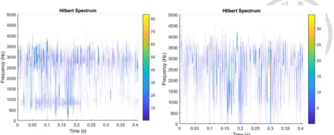
Fig. 12 shows the 11 IMFs that are decomposed from a cutting signal. Fig. 13 shows that Hilbert transform extracts the envelope of the signal, as shown in the red dotted curve. We can define 𝐸_𝐻𝐻𝑇 = |𝑥_𝑛(𝑡)/𝑥(𝑡)|² as the energy for the HHT result, where 𝑥_𝑛(𝑡) is the 𝑛-th IMF and 𝑥(𝑡) is the original vibration signal. Fig. 14 is the time- frequency visualization of the spectrum obtained using HHT. It’s also possible to extract the chatter frequency band by applying WPT to the input signal, take the wavelet coefficients from the chatter frequency band, and apply inverse WPT. Then the signal can be processed with HHT to get the energy of each IMF. This approach has been shown to be more effective than using HHT alone [32]. In this research, we set 𝑛 = 1, which implies 𝐸_𝐻𝐻𝑇 is high when the first IMF has large amplitudes.

(32)

Fig. 12. IMFs of a cutting signal obtained using HHT

Fig. 13. Illustration of Hilbert transform on vibration signal [67]

(33)

Fig. 14. Hilbert spectrum of unstable (left) and stable (right) cutting signals calculated and visualized with MATLAB

(34)

3. Classification algorithms

After we obtain the feature vectors using the signal processing methods described in the previous chapter, they will be put into a classification algorithm to train a model. The model will be able to predict whether a signal belongs to stable or unstable. Since our dataset is labeled, we mainly focused on supervised learning. In this chapter, several methods and classification algorithms are used, and their effectiveness are compared.

The simplest method is to set a fixed threshold value to distinguish stable data from the unstable ones. A statistical method – Naïve Bayes was tested in 3.2. Some commonly used classification algorithms, such as local outlier factor (LOF), support vector machine (SVM), and k-nearest neighbor (k-NN), were applied to our dataset. Finally, we utilized artificial neural network (ANN) to obtain models for prediction.

3.1 Numerical threshold

Using a fixed threshold as the boundary of stable and unstable region is one of the simplest and most straightforward method. This method relies on the distribution of a feature to be separable by a single threshold. The calculation steps are as follows:

1. Choose a feature that is represented by a single numerical value, e.g. the relative energy after FFT of the x-axis signal.

2. Compute the values of this feature for the entire dataset to obtain the distribution of both stable and unstable data.

3. Let there be m stable data points and n unstable data points. Since relative energy is larger for unstable data points, choose the m-th smallest value in these 𝑚 + 𝑛 data points. This is the selected threshold. A data point is considered

(35)

3.2 Naïve Bayes

Naïve Bayes is a probabilistic classifier based on Bayes’ theorem, widely used in machine learning [68] [69] [70]. The general idea is as follows. Given a set of features, such as the energy ratios of x-, y-, and z-axis, we know the distribution of each feature for both unstable and stable data. Then, we fit the distribution curve with, e.g. Gaussian distribution. Now, given a new data point, we can estimate its probability of being unstable based on the fitted distribution and its energy ratio from x-axis. Same can be done with y- and z-axis.

Given a feature vector 𝐱 = (𝑥₁,… ,𝑥_𝑛) , and classes {𝐶_𝑘} , we want to calculate 𝑝(𝐶_𝑘|𝑥₁,… ,𝑥_𝑛), the probability that x belongs to Ck , for each k. To determine which class 𝐱 belongs to, we want to find k that maximizes 𝑝(𝐶_𝑘|𝑥₁,… ,𝑥_𝑛). Assume all features x1, … , xn are independent. By Bayes' theorem,

𝑝(𝐶_𝑘|𝐱) =𝑝(𝐶_𝑘)𝑝(𝐱|𝐶_𝑘)

𝑝(𝐱) .

By chain rule,

𝑝(𝐶_𝑘|𝐱) ∝ 𝑝(𝐶_𝑘, 𝑥₁, … , 𝑥_𝑛) = 𝑝(𝐱|𝐶_𝑘) = 𝑝(𝐶_𝑘)𝑝(𝑥₁|𝐶_𝑘) … 𝑝(𝑥_𝑛|𝐶_𝑘),

where 𝑝(𝐶_𝑘) is called prior probability, or simply prior. For our application, we set 𝑝(𝐶_𝑘) = 1/𝑘 for all k. 𝑝(𝑥₁|𝐶_𝑘) depends on the model fitting methods, such as Gaussian or Bernoulli.

(36)

3.3 Local outlier factor (LOF)

LOF is an algorithm to distinguish outliers from clusters of data points, and has been used in audio and image recognition [71]. Previous work used LOF to classify relative wavelet packet entropy [72]. To use this method in this research, it is required to limit the ratio of unstable data points so that they are significantly less than the stable once. This is because LOF finds the outliers, i.e. the points far away from other points.

Define k-distance 𝑘(𝐴) be the k-th nearest neighbor of point A. Denote the distance between two points A and B as 𝑑(𝐴, 𝐵). Define reachability distance as

𝑟_𝑘(𝐴, 𝐵) = 𝑚𝑎𝑥{𝑘(𝐵), 𝑑(𝐴, 𝐵)}.

The reason to use reachability distance instead of the distance between A and B is to get more stable results in computations. Furthermore, define local reachability density as

𝑙𝑟𝑑_𝑘(𝐴) = |𝑁_𝑘(𝐴)|

∑_𝐵∈𝑁 𝑟_𝑘(𝐴, 𝐵)

𝑘(𝐴)

,

where 𝑁_𝑘(𝐴) is the k nearest neighbors of A. Roughly speaking, local reachability density is the reciprocal of the average distance between A and its neighbors. The local outlier factor is

𝐿𝑂𝐹_𝑘(𝐴) =

∑ 𝑙𝑟𝑑(𝐵)

𝑙𝑟𝑑(𝐴)

𝐵∈𝑁_𝑘(𝐴)

|𝑁_𝑘(𝐴)| = ∑_𝐵∈𝑁_𝑘_(𝐴)𝑙𝑟𝑑(𝐵)

|𝑁_𝑘(𝐴)| ∙ 𝑙𝑟𝑑(𝐴).

(37)

Fig. 15. An example of visualized local outlier factors

3.4 Support vector machine (SVM)

SVM is a well-known method to separate two classes of data points [73] [74], and has the advantage of good performance because the equations can be written in linear form. SVM has been used for chatter recognition when combined with information entropy [75], WPT [76], and Q-factor [77].

There are two types of SVMs, linear and non-linear. For linear SVM, suppose there are n points (𝐱_𝟏, 𝑦₁), … , (𝐱_𝐧, 𝑦_𝑛), where 𝑦_𝑖 = ±1, SVM attempts to separate the points with 𝑦_𝑖 = 1 from the ones with 𝑦_𝑖 = −1 using a hyperplane 𝐰 ∙ 𝐱 − 𝑏 = 0 with some vector 𝐰, called support vector. This is illustrated in Fig. 16 (a). In practice, there are cases when the points cannot be separated by a hyperplane as in Fig. 16 (b). In such cases, the points are mapped to higher dimensional space using a kernel function such as

(38)

polynomial, RBF, and sigmoid. The mapped points may be easily separable with a hyperplane.

(a)

(b)

Fig. 16. (a) Illustration of linear SVM for a linearly-separable dataset [78] (b) Non- linear SVM with RBF kernel [79]

(39)

3.5 K-nearest neighbor (k-NN)

K-NN is a simple classification algorithm based on votes from the neighbors [80].

Suppose we have a data point A without knowing whether it is stable or unstable. We find k-nearest neighbors of A for some k. Let’s say 𝑘 = 5, and there are 3 of them are stable, and 2 are unstable. Since 3 2, k-NN classify A as stable.

It is easy to add a weight function 𝑤(𝑟) for each neighbor. For example, let the k neighbors of A be 𝑝₁, … , 𝑝_𝑘, and the first m points are stable while the rest are unstable.

Let the distance between A and 𝑝_𝑖 be 𝑟_𝑖 for all i. Then, define the scores

𝑠𝑐𝑜𝑟𝑒(𝑠𝑡𝑎𝑏𝑙𝑒) = ∑ 𝑤(𝑟_𝑖)

𝑚

𝑖=1

𝑠𝑐𝑜𝑟𝑒(𝑢𝑛𝑠𝑡𝑎𝑏𝑙𝑒) = ∑ 𝑤(𝑟_𝑖)

𝑘

𝑖=𝑚+1

If 𝑠𝑐𝑜𝑟𝑒(𝑠𝑡𝑎𝑏𝑙𝑒) 𝑠𝑐𝑜𝑟𝑒(𝑢𝑛𝑠𝑡𝑎𝑏𝑙𝑒), then A should be classified as stable, and vice versa. Some common weight functions 𝑤(𝑟) are 1 (uniform), 𝑟^−𝑎, and 𝑒^−𝑎, for some 𝑎 0.

(40)

3.6 Artificial neural network (ANN)

Using ANN in chatter recognition has the advantage that a detailed model is not required and reasonable accuracy may still be achieved without manually select an optimal feature as input. For this reason, we will use the entire frequency spectrum as the input of the ANN. The vibration signal will be converted into frequency domain using FFT, and ANN should be able to distinguish the stable data from unstable data since chatter is more easily recognizable in frequency domain. The architecture and training parameters will be manually tuned to obtain a good accuracy.

(41)

4. Implementation

4.1 Architecture of the data analysis and model training platform

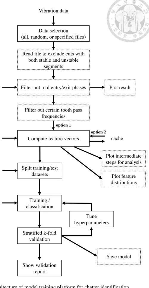
Fig. 17 shows the architecture of the model training platform developed in this research. This platform makes it easy to change the feature or classification algorithm to use, adjust the corresponding parameters, and quickly obtain a validation report

indicating the effectiveness of the trained model. Any combination of the mentioned features and classification algorithms can be used, along with several modes for tool entry/exit detection, data selection, etc.

The blocks with solid lines in Fig. 17 indicates a data processing or calculation step. A block with dashed lines represents an optional step. First, vibration data from the accelerometer, along with their labels, are loaded from files. Then, the tool entry and exit parts of the vibration signals are excluded to ensure the data being trained are valid cutting data. Certain tooth pass frequencies that are too close to chatter frequencies are filtered out to prevent misidentifications. Features are then computes according to the specified parameters, and saved into a cache file so that if the same feature is to be used again with another classification algorithm, we can simply load all features from cache.

This can drastically reduce the computation time. Therefore, we have two data sources:

from file (option 1) and from cache (option 2).

The dataset, consisting of feature vectors and labels, is then split into training and test datasets randomly. Models are trained and validated using stratified k-fold

validation. Some hyperparameters are automatically tuned to minimize error rate. The validation report of the final model will be shown to summarize the results.

(42)

Fig. 17 Architecture of model training platform for chatter identification Vibration data

Data selection

(all, random, or specified files)

Read file & exclude cuts with both stable and unstable

segments

Filter out tool entry/exit phases Tool entry/exit

detection mode Plot result

Filter out certain tooth pass frequencies

Selected feature

& parameters Compute feature vectors cache

option 1

option 2

Plot intermediate steps for analysis Split training/test

datasets k-fold validation

parameters Plot feature

distributions Classification

algorithm &

parameters

Training / classification

Stratified k-fold validation

Tune hyperparameters

Save model Show validation

report

(43)

4.2 Implementation details

This section will describe the techniques used to implement the model training platform shown in Fig. 17. The entire program is written in Python 3. The main libraries that was used is listed in Table 1.

Table 1. Major libraries used to implement the platform

library Main usage in our platform

numpy High performance numerical computations

scipy FFT, filters

PyWavelets WPT

pyhht HHT

matplotlib Data visualizations

scikit-learn LOF, k-NN

keras ANN

tensorflow ANN

4.2.1 Zero-padding before FFT

Our program uses numpy for FFT computations. For some testing data, performance issues were observed. After some investigations, the conclusion is the implementation of numpy’s fft.rfft() function is the cause of the issue. When the length of input array is not an integer power of 2, it tries to factor the length and split the computation into chunks. However, when the length is a prime number, the computation slows down drastically. As we can see in Table 2, the computation time when the array length is 16384 (= 2¹⁴) is better than 12581 (= 23×547) and 12584 (= 2³×11²×13), and more than 50 times better than 12583, which is a prime number.

A technique called zero-padding can be applied to resolve this issue. We zero- pad the original vibration signal to so that the total length is an integer power of 2. For example, if the vibration signal has 12583 samples, we add zeros to the array until the length is 16384. This can significantly improve performance while not negatively

(44)

affecting the frequency spectrum of the FFT output. In fact, zero-padding improves the frequency resolution of the output spectrum. Note that when window function is used, the signal should be zero-padded before applying a window function.

Table 2. Performance test on numpy.fft.rfft()

Input array length Computation time (sec)

12581 0.01698

12582 0.00898

12583 0.48424

12584 0.01039

16384 0.00937

32768 0.01051

65536 0.01897

4.2.2 Computing autocorrelation coefficients

The time complexity of direct computation of autocorrelation coefficients from (4) is O(N²). However, this can be improved to O(N log N) using FFT because (4) is similar to the equation of discrete convolution

(𝑓 ∗ 𝑔)[𝑛] = ∑ 𝑓[𝑚]𝑔[𝑛 − 𝑚].

𝑁

𝑛=−𝑁

Fig. 18 shows how discrete convolution can be computed in O(N log N) instead of O(N²) for the direct approach. We show the connection between (4) and the equation above below.

(45)

Fig. 18. Illustration of the computation of discrete convolution

Proposition Given two 0-indexed arrays x and y, of length Nx and Ny respectively.

Define discrete convolution as

(𝑥 ∗ 𝑦)[𝑚] = ∑ 𝑥[𝑛]𝑦[𝑚 − 𝑛]

𝑁𝑦−1

𝑛=0

for m ∈ [0, 𝑁_𝑥+ 𝑁_𝑦− 2], (7)

and assume x[i] = y[i] = 0 for i < 0. Let z be the reversed array of x, i.e. 𝑧[𝑖] = 𝑥[𝑁_𝑥− 𝑖 − 1] for all i. Then,

(𝑧 ∗ 𝑥)[𝑚 + 𝑁 − 1] = ∑ 𝑥[𝑛]𝑥[𝑚 + 𝑛]

𝑁−1

𝑛=0

, (8)

proof

(𝑧 ∗ 𝑥)[𝑚]

= ∑ 𝑧[𝑛]𝑦[𝑚 − 𝑛] (𝑏𝑦 (7))

𝑁_𝑦−1

𝑛=0

𝑓 ∗ 𝑔 𝑛 = ∑ 𝑓 𝑚 𝑔[𝑛 − 𝑚]

𝑁

𝑛=−𝑁

𝑓, 𝑔 O(N²) 𝑓 ∗ 𝑔

Direct computation

FFT

𝐹, 𝐹

Multiplication

O(N)

O(N log N) Inverse FFT O(N log N)

(46)

= ∑ 𝑧[𝑁_𝑦− 1 − 𝑝]𝑦[𝑚 + 𝑝 + 1 − 𝑁_𝑦] (𝑝 = 𝑁_𝑦− 1 − 𝑛)

𝑁_𝑦−1

𝑝=0

= ∑ 𝑥[𝑝] 𝑦[𝑚 + 𝑝 + 1 − 𝑁] (𝑏𝑦 (2), 𝑎𝑛𝑑 𝑙𝑒𝑡 𝑁 = 𝑁_𝑥 = 𝑁_𝑦)

𝑁−1

𝑝=0

= ∑ 𝑥[𝑛] 𝑦[(𝑚 + 1 − 𝑁) + 𝑛]

𝑁−1

𝑛=0

Substituting m with m+N-1, we get (8).

The above proposition can be directly applied because (7) matches the implementation of scipy’s fftconvolve. Specifically, (𝑥 ∗ 𝑦) = fftconvolve(x, y, mode=‘full’).

4.2.3 Peak finding

Peak finding is used in parts of the program, e.g. finding n-highest peaks in the spectrums after FFT, and finding peaks in autocorrelation coefficient plot. We used 𝑠𝑐𝑖𝑝𝑦. 𝑠𝑖𝑔𝑛𝑎𝑙. 𝑓𝑖𝑛𝑑_𝑝𝑒𝑎𝑘𝑠 to implement these parts of the program. The parameters used include the minimum horizontal distance between peaks, and prominence.

When trying to find peaks within a graph, e.g. a spectrum, the minimum horizontal distance between peaks is set to ensure that two peaks very close to each other won’t be both included in the result. Suppose 20 peaks should be selected from a vibration signal spectrum, there may be 3 peaks near one tooth pass frequency. The unintended

(47)

consequence is that probably only 7 tooth pass frequencies are included in the 20 peaks that the algorithm found, instead of 20.

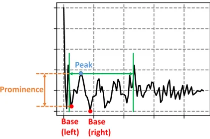
Prominence is a property of a peak, describing the height of a peak relative to the neighboring values. The calculation of prominence is as follows:

(1) Draw a horizontal line, crossing the peak in discussion, until it intersects the signal or the window border. This is illustrated by the green lines in Fig. 19.

(2) For the left and right sides of the peak, find the minimum of each side, these are the bases of the peak as shown in red dots in Fig. 19.

(3) The prominence is the difference between the height of the peak and the higher value of the bases.

Therefore, it is possible to find n most prominent peaks from a graph by ordering the prominences of all peaks, and take the largest n results. This concept is used in the implementation of autocorrelation coefficients.

Fig. 19. Illustration of the peak finding procedure and the calculation of prominence of a peak

Peak

Base (left)

Base (right) Prominence

(48)

4.3 Validation

In machine learning, training and test datasets must be separated. Otherwise, it is trivial to obtain a model that achieves 100% accuracy for supervised learning – simply memorize all data and their labels and build a lookup table. To evaluate the true accuracy of a model, we use one of the standard approaches – stratified k-fold validation. The concept is shown in Fig. 20 for the case 𝑘 = 3, where the dataset is split into 3 parts. There are k rounds of validations. For the first round, the first 1/𝑘 data are used for training while the rest are used for testing. Note that each the ratios of A and B classes in each 1/𝑘 part should be identical.

In this research, the dataset consists vibration data from 143 cuts. Each cut may result in many data points due to the sliding window we use. However, during the learning and validation process, if a cut is used for training, all data points in that cut are used as training, and vice versa. This ensures the result is fair and minimizing overfitting.

Fig. 20. Illustration of stratified k-fold validation [47]

(49)

5. Results and discussion

5.1 Data collection and labeling

The experiment data of this research comes from previous work of our laboratory [47]. Since the goal of this research is chatter identification, a sufficient number of experiment data is required as inputs for classification algorithms. Our dataset contains vibration signals from a CNC milling machine, while cutting at different spindle speed, depth of cut, and feed rates. Stability lobe diagram (SLD) of the CNC machine was obtained by the traditional method - modal test and cutting force coefficients measurement. The cutting conditions, which includes spindle speed, depth of cut, and feed rate, were chosen so that it is near the stability boundary of the SLD. SLD is not necessary, but it makes it easier to search for cutting conditions that is in the stable or unstable region.

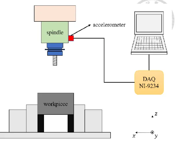
We used a CNC milling machine to perform the cutting experiment. The experiment setup is shown in Fig. 21. A tri-axial accelerometer was mounted on the spindle housing, and NI-9234 DAQ was used at sampling rate of 10240 Hz to acquire the vibration signals. 143 straight cuts were performed and each cut lasts around 5 seconds, excluding tool entry and exit phase. These 143 cuts contain at least 110 spindle speed and depth of cut combinations, so we have good variety in our dataset. While conducting the experiment, we labeled whether chatter occurs during this cut by listening to the sound.

There are 3 possible values for this label – entirely stable, entirely unstable, and partially unstable. Therefore, the dataset consists of vibration signals from 143 cuts, along with a label.

(50)

Fig. 21 Experiment setup when gathering the dataset

Accelerometer was installed on the spindle housing, and a NI DAQ was used to acquire the signal. [47]

5.2 Comparisons of classification algorithms

In this section, different classification algorithms are compared using the same feature. The feature used is FFT energy ratio, 𝐸_{1,𝐹𝐹𝑇}, with window size of 1.2 seconds, no overlap, exponent of 2.75, and all three axes. Since the window and overlap are fixed, the number of data points used to train the models are identical, giving a fair comparison of different classification algorithms.

(51)

The numeric threshold method yields an error rate of 6.579%, with false alarm and missing alarm rates both being 3.289%. Naïve Bayes produces error rates of 5.263%

and 5.482% using Gaussian and Bernoulli Naïve Bayes, respectively.

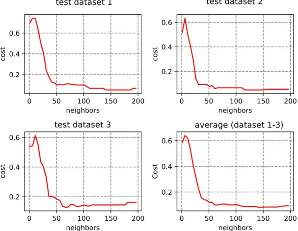
Fig. 22 shows the testing cost when using LOF as the classifier. Using stratified k-fold validation with 𝑘 = 3, the cost of 3 test datasets are shown, with the average at the bottom-right corner. In terms of error rate, the optimal amount of neighbors is approximately 150. The cost varies between 0 to 1, with 0 meaning all data points are correctly classified, and 1 meaning all are incorrectly classified. Also, since the unstable data point ratio is an adjustable parameter, the relation between it and error rate is listed in Table 3, where using 15% of unstable data is optimal with an error rate of 8.53%.

Fig. 22. Test costs of LOF for each of the three test datasets, and the average costs

(52)

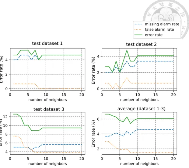
Fig. 33 shows the error rates on three test datasets and the average using k-NN as the classifier. Table 4 shows the error rates with different weights, including uniform, 𝑟^−𝑎, and 𝑒^−𝑎𝑟 with some 𝑎. The lowest error rate is 5.21% while the highest is 6.061%.

The difference is small, which leads to the conclusion that the weight does not affect the error rate significantly.

Fig. 24 sums up this section with all optimal error rates from each classification method compared. K-NN is the best one at 5.21%, almost matched by Naïve Bayes at 5.263% and SVM at 5.647%. Numeric threshold and LOF are the worse ones. Incidentally, an error rate of 7.12% is achieved using ANN, placing it as the 5th best feature. However, since the methodology of it is quite different to other classification methods, it is best to not make direct comparison.

Table 3. Classification error rates using FFT (𝐸_{1,𝐹𝐹𝑇}) and different unstable data point ratio in LOF

Unstable data point ratio (%) ER (%)

10 10.4 (14.8)

15 8.53 (14.4)

20 9.01 (18.1)

Feature: [window=1.2, overlap=0, exp=2.75, bw=10, xyz], classification: [LOF, auto[1-200], weight 1/r^3]

(53)

Fig. 23. Test error rates of K-NN for each of the three test datasets, and the average error rates.

(54)

Table 4. Classification error rates using k-NN and different weights

Weight FA (%) MA (%) ER (%)

uniform 0.646 (1.258) 5.222 (6.918) 5.868 (8.176)

𝑟⁻¹ 1.065 (2.516) 4.564 (6.289) 5.629 (8.805)

𝑟⁻² 1.275 (3.145) 4.354 (5.66) 5.629 (8.805)

𝑟⁻³ 1.485 (3.774) 4.576 (5.66) 6.061 (9.434)

𝑟⁻⁴ 1.48 (3.774) 4.349 (5.66) 5.829 (9.434)

𝑒^−𝑟 0.646 (1.258) 5.222 (6.918) 5.868 (8.176)

𝑒^−2𝑟 0.646 (1.258) 5.222 (6.918) 5.868 (8.176)

𝑒^−5𝑟 0.646 (1.258) 4.773 (6.918) 5.419 (8.176)

𝑒^−10𝑟 0.8557 (1.887) 4.354 (5.66) 5.21 (7.547)

𝑒^−100𝑟 2.096 (6.289) 3.691 (5.031) 5.787 (11.32) Feature: [window=1.2, overlap=0, exp=2.75, bw=10, xyz], classification: [knn, auto[1-200], weight 1/r^3]

(55)

Fig. 24. Error rates when different classification methods are used with the same feature (FFT relative energy)

5.3 Parameters optimizations

This section is focus on parameter optimization for each feature extraction method.

For example, the parameters involved in WPT includes mother wavelet, window and overlap sizes, and exponent used to compute the energy. We will find the optimal values for these parameters to obtain the best error rate for WPT, and in later sections this error rate can be compared to other feature types, such as autocorrelation coefficients, to give a fair comparison of the effectiveness of different features.

0 2 4 6 8 10

Threshold LOF Naïve Bayes

k-NN SVM

Error rate (%)

(56)

5.3.1 Fast Fourier transform (FFT)

This section describes the classification results when using FFT-related features, and FFT parameter optimizations will be discussed. The first feature we investigate is the relative energy 𝐸_{1,𝐹𝐹𝑇}. The exponent 𝑝 in (1) is an adjustable parameter, and can take any value in (0, ∞). Fig. 25 illustrates the spectrum amplitudes |𝑆(𝑓)|^𝑝 for 𝑝 = 0.5, 1, 2.75, and 8. Top right figure is for 𝑝 = 1, i.e. the original FFT spectrum. The highest peak at around 900 Hz is the chatter frequency of the machine. There are several smaller peaks at tooth pass frequencies. In addition, the noise is can be clearly seen in the spectrum as well, especially in the frequency range of 2000 to 3500 Hz. These unwanted noise is sometimes unavoidable and may negatively impact the detection of chatter. We argue that the parameter 𝑝 can reduce the effect of noise.

When we increase the value of 𝑝 to 2.75, the smaller peaks become smaller relative to the dominant chatter peak. Due to their smaller amplitudes, the noise between 2000 to 3500 Hz become significantly lower relative to the chatter and tooth pass frequency peaks. If 𝑝 is further increased to 8 as shown in the bottom right figure, only 2 largest peaks are visible. This is not ideal because most of the information in the spectrum is lost, and classification error rate will increase. On the other hand, using 𝑝 < 1 increases the influence of smaller peaks and amplifies the noise. In summary, there are adverse effects when 𝑝 is too large or too small. We aim to find an optimal value.