對磁聲波觸發前恆星核塌縮之模擬

(1)

國立臺灣大學理學院天文物理研究所碩士論文

Graduate Institute of Astrophysics College of Science

National Taiwan University Master Thesis

對磁聲波觸發前恆星核塌縮之模擬

Simulating the Collapse of Prestellar Cores Triggered by Magnetosonic Waves

黃彥凱 Yen-Kai Huang

指導教授：闕志鴻　博士 Advisor: Tzihong Chiueh, Ph.D.

中華民國 106 年 7 月

July, 2017

(2)

(3)

(4)

(5)

誌謝

這份論文得以完成，首先要感謝闕志鴻教授的指導，在面對各種問題及困難時，教授總是能夠維持理性、客觀的態度去處理，是我在學術研究上所不足的。再來我必須要感謝實驗室的大學長瑋瀚，不管是對物理系統的看法還是軟體硬體的問題，我都從你獲得了很多的幫助，

能夠快速地對 GAMER 上手，很大一部分是托你的福！闕老師實驗室的大家，翔哥、家榮、姝蓉學姊、小于學長、家豪、若有、冠維、弘旭學長、善長、彥麟學長以及慧敏，還有機器們，與你們經歷了兩個寒暑，這些日子非常深刻，希望未來在各自的路上都能穩定前進。當然，在天數 922 中，許多陪我一起度過研究生日子的戰友，文斌、聖傑、瑀潔、芝寅哥、濟家學長、偉良、柏文、Kota，與前面提過的翔哥和家榮，如果沒有你們，這段研究生活恐怕會變得相當苦悶吧，很開心認識了你們！

當然，還要感謝媽在我就讀研究所的這段時間，儘管過程有些顛簸，您從不過問及干涉，總是照顧好生活中的一切，放心地讓我自己做出抉擇，從小到大，我對您有道不盡的感謝。此外，還有生活中的朋友們，總是一起吃飯的阿虛、思羽、吃吃、火星，天文社圈子的阿尖、育瑋、小光，老朋友們老白和怡臻，以及其他許許多多的人們，

很感謝你們陪我走過了這段時光。

最後，我要感謝老婆琬婷，這些日子以來，我們一起笑、一起分擔悲傷、一起度過困難，妳真誠而率性，雖然我們偶有摩擦，但與妳相處的時光，是獨一無二的。大學生活、碩士時期，我真的非常幸運能有妳在我身旁，未來的日子，也要請妳多多指教了！

(6)

(7)

摘要

於此研究我們分析由環境中波狀擾動所觸發的前恆星核的塌縮。

在前人的研究結果中，不考慮磁場及旋轉所造成的效應下，模擬結果顯示當波狀擾動以脈波的形式撞擊核心，脈波的振幅大於背景值的

∼ 2.5% 時，便足以在最適條件下造成核心塌縮。藉由將延伸至理想磁 流體系統的鬆弛全差變遞減方法套用到 GAMER 程式碼中，我們得以考慮背景磁場對上述波致塌縮機制的影響。另外，考慮到系統中發生的加熱及冷卻效應，我們使用了兩種特別的狀態方程，它們最大的特點在於所牽涉的絕熱指數具有密度的相依性。

在背景磁場的影響下，進入完全鬆弛狀態的核心其形狀改變為一扁平橢球，而當我們不考慮磁場造成的效應，原本的球狀核心在鬆弛過程中不改變它的形狀。對於完全鬆弛的核心，我們用脈波撞擊之。當脈波到達核心時，它會在核心外表面產生向內傳播的橢圓震波，如果脈波夠強，這些震波的匯聚就足以造成核心的塌縮。對此機制來說，

若使用第一種狀態方程，最適頻率落在 ν/ν₀ = 4.5；而當我們使用第

二種狀態方程，最適頻率則會減小至 ν/ν₀ = 1.5。

當脈波以垂直背景磁場的方向撞擊核心，若要導致塌縮，脈波的 振幅需有背景值的 16.5%，這比我們不考慮磁場效應的對應組還多了

∼ 30%。同時若脈波傳遞方向與背景磁場重合，波致塌縮機制的效率 亦會顯著減小。最後，藉由將我們波致塌縮模擬的結果與前人相比較，

兩者波致塌縮的過程差異讓我們對此機制有更深入的了解。

關鍵詞：磁流體力學、恆星形成、前恆星系統、類太陽恆星、數值模擬。

(8)

(9)

Abstract

We analyze the collapse of isolated starless cores triggered by the impingement of wave-like perturbations. Previous work has shown that in the absence of the magnetic field and the initial rotation, a Gaussian sound pulse with its amplitude at least∼ 2.5% relative to the ambient gas can set off the collapse in the optimal case. By implementing the ideal MHD extension of relaxing TVD (RTVD) scheme into the GAMER code, we study this collapse mechanism regarding the magnetic interplay and the core rotation. To model the heating and cooling effects, we apply two types of the equation of state (EOS) that the adiabatic index is density-dependent.

In the magnetic cases, the fully-relaxed core is a oblate spheroidal, while the spherical shape is retained in the non-magnetic case. Different Gaussian fast pulses are then launched toward the cores. On its arrival, the pulse generates inward spheroidal shocks on the core surface. The convergence of the shock fronts results in the core collapse provided the pulse is strong enough.

The favorite frequency of the mechanism is ν/ν₀ = 4.5 when the type 1 EOS is applied. In the cases of the type 2 EOS, the favorite frequency shifts to a smaller value, ν/ν0 = 1.5.

For a pulse propagating perpendicular to the background magnetic field, the required pulse amplitude is 16.5% relative to the ambient, ∼ 30% more than the corresponding value in the non-magnetic case. Meanwhile, the align- ment between the pulse propagating direction and the magnetic field lines substantially decreases the efficiency of the material compression. Finally,

(10)

we compare our results to the previous work to gain more insights into the nature of the wave-triggered collapse.

Key words: magnetohydrodynamics, star formation, prestellar systems, solar-luminous stars, numerical simulation

(11)

List of Figures

2.1 CPU + GPU cooperation in GAMER . . . 9

2.2 Flow chart of the RTVD scheme . . . 12

2.3 Schematic picture of the variable centering . . . 13

3.1 Initial conditions before the core relaxation . . . 17

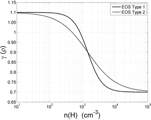
3.2 The density dependence of γ(ρ) for the two types of the equation of state. Typical hydrogen number density n(H) is 10⁴ cm⁻³ for the core and 20 cm⁻³for the ambient gas. . . 19

4.1 Peak density evolution of the relaxing cores. The peak density has been normalized to the initial value for each model. . . 25

4.2 Peak density evolution of the relaxing cores during the last few oscillatory periods. The peak density has been normalized to the initial value for each model. . . 26

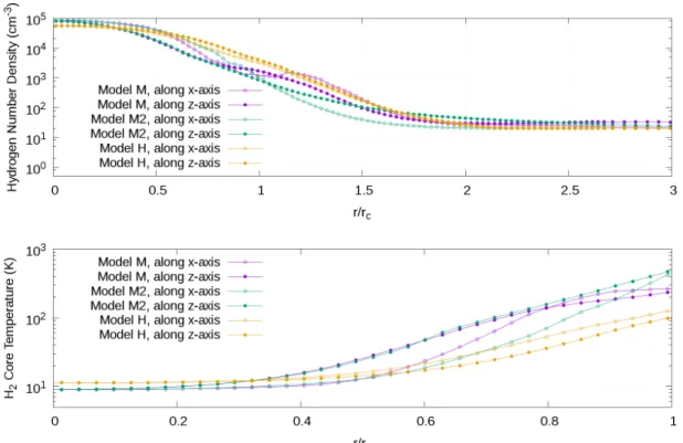
4.3 The core profile after the relaxation process. Top panel: the hydrogen number density profile from r = 0–3 r_c. Bottom panel: the H₂ core tem- perature within r = r_c. . . 27

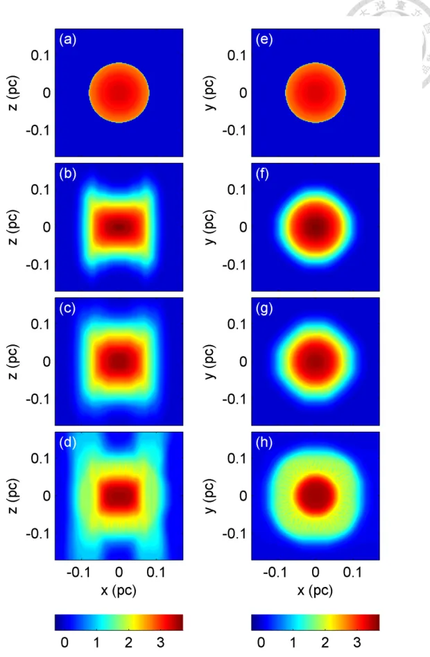
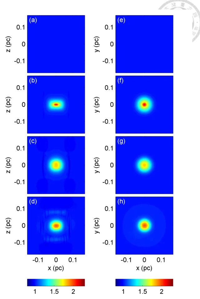
4.4 The log₁₀|ρ| contour maps (normalized to the ambient gas value) during the relaxation process in Model M. From top to bottom, the core has experienced 0, 8, 17, and 43 oscillatory periods. Figure (a) – (d) show the y = 0 plane near the core, while figure (e)–(h) are the z = 0 plane near the core. . . 29

(14)

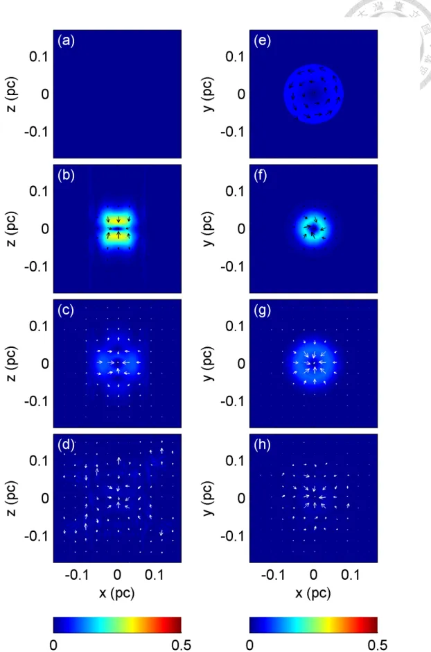
4.5 The poloidal velocity field during the relaxation process in Model M. The magnitude is in the unit of local √

c²_S+ c²_A and arrows represent the direction. From top to bottom, the core has experienced 0, 8, 17, and 43 oscillatory periods. Figure (a) – (d) show the y = 0 plane near the core, while figure (e)–(h) are the z = 0 plane near core. . . . 30 4.6 The total pressure (normalized to the ambient gas value) during the relax-

ation process in Model M. From top to bottom, the core has experienced 0, 8, 17, and 43 oscillatory periods. Figure (a) – (d) show the y = 0 plane near the core, while figure (e)–(h) are the z = 0 plane near the core. . . . 31 4.7 The poloidal magnetic field (normalized to the initial magnetic strength)

during the relaxation process in Model M, with arrows representing the direction. From top to bottom, the core has experienced 0, 8, 17, and 43 oscillatory periods. Figure (a) – (d) show the y = 0 plane near the core, while figure (e)–(h) are the z = 0 plane near the core. . . . 32 4.8 The log10|ρ| contour maps (normalized to the ambient gas value) during

the relaxation process in Model M2. From top to bottom, the core has experienced 0, 8, 17, and 38 oscillatory periods. Figure (a) – (d) show the y = 0 plane near the core, while figure (e)–(h) are the z = 0 plane near the core. . . 33 4.9 The poloidal velocity field during the relaxation process in Model M2.

The magnitude is in the unit of local√

c²_S+ c²_Aand arrows represent the direction. From top to bottom, the core has experienced 0, 8, 17, and 38 oscillatory periods. Figure (a) – (d) show the y = 0 plane near the core, while figure (e)–(h) are the z = 0 plane near the core. . . . 34 4.10 The total pressure (normalized to the ambient gas value) during the relax-

ation process in Model M2. From top to bottom, the core has experienced 0, 8, 17, and 38 oscillatory periods. Figure (a) – (d) show the y = 0 plane near the core, while figure (e)–(h) are the z = 0 plane near the core. . . . 35

(15)

4.11 The poloidal magnetic field (normalized to the initial magnetic strength) during the relaxation process in Model M2, with arrows representing the direction. From top to bottom, the core has experienced 0, 8, 17, and 38 oscillatory periods. Figure (a) – (d) show the y = 0 plane near the core, while figure (e)–(h) are the z = 0 plane near the core. . . . 36 4.12 The log₁₀|ρ| contour maps (normalized to the ambient gas value) during

the relaxation process in Model H. From top to bottom, the core has experienced 0, 8, 19, and 58 oscillatory periods. Figure (a) – (d) show the y = 0 plane near the core, while figure (e)–(h) are the z = 0 plane near the core. . . 37 4.13 The poloidal velocity field during the relaxation process in Model H. The

magnitude is in the unit of local c_S and arrows represent the direction.

From top to bottom, the core has experienced 0, 8, 19, and 58 oscillatory periods. Figure (a) – (d) show the y = 0 plane near the core, while figure (e)–(h) are the z = 0 plane near the core. . . . 38 4.14 The total pressure (normalized to the ambient gas value) during the relax-

ation process in Model H. From top to bottom, the core has experienced 0, 8, 19, and 58 oscillatory periods. Figure (a) – (d) show the y = 0 plane near the core, while figure (e)–(h) are the z = 0 plane near the core. . . . 39 4.15 The evolution of the ρv_ϕ (normalized to the initial r = r_c value) during

the relaxation process. All the figures are the y = 0 plane near the core. In figure (a)–(d) the core has experienced 0, 8, 17, and 43 oscillatory periods in model M, while in figure (e)–(h) the core has experienced 0, 8, 19, and 58 oscillatory periods in model H. . . 40 4.16 The evolution of the ρv_ϕ (normalized to the initial r = r_c value) during

the relaxation process. All the figures are the y = 0 plane near the core. In figure (a)–(d) the core has experienced 0, 8, 17, and 38 oscillatory periods in model M2, while in figure (e)–(h) the core has experienced 0, 8, 19, and 58 oscillatory periods in model H. . . 41

(16)

4.17 Core phase during the pulse impingement in the optimal cases. The lower bar and the point represent the moment that the pulse contacts with the

core boundary and reaches the core center, respectively. . . 44

4.18 The log₁₀|ρ| contour maps (normalized to the ambient gas value) in Model PM90. From top to bottom, the pulse is initially launched, just contacts with the core boundary, has almost left the core, and is faraway from the core. Figure (a) – (d) show the y = 0 plane near the core, while figure (e)–(h) are the z = 0 plane near the core. . . . 45

4.19 The log₁₀|ρ| contour maps (normalized to the ambient gas value) in Model PM0. From top to bottom, the pulse is initially launched, just contacts with the core boundary, has almost left the core, and is faraway from the core. Figure (a) – (d) show the y = 0 plane near the core, while figure (e)–(h) are the z = 0 plane near the core. . . . 46

4.20 The log10|ρ| contour maps (normalized to the ambient gas value) in Model PH. From top to bottom, the pulse is initially launched, just contacts with the core boundary, has almost left the core, and is faraway from the core. Figure (a) – (d) show the y = 0 plane near the core, while figure (e)–(h) are the z = 0 plane near the core. . . . 47

4.21 Frequency-phase diagram for model PM90 . . . 48

4.22 Frequency-phase diagram for model PM0 . . . 48

4.23 Frequency-phase diagram for model PH . . . 49

4.24 Frequency diagram for model PM90, model PM0, and model PH . . . 49

5.1 (a) The log₁₀|ρ| (normalized to the ambient gas value) and (b) the log10|vpol| (in the unit of local√ c²_S+ c²_A) contour maps when the core has experienced 8 oscillations in model M. The arrows represent the direction of v_pol. . . 52

5.2 The log10|vpol| (in the unit of local√ c²_S+ c²_A) contour maps when the core has experienced (a) 0.008, (b) 0.016, and (c) 0.16 oscillations in model M. The arrows represent the direction of v_pol. . . 52

(17)

5.3 The gas pressure (normalized to the ambient gas value) contour maps when the core has experienced 43 oscillations in model M. (a) y = 0 slice (b) z = 0 slice (c) z ∼ 0.028 pc slice (d) z ∼ 0.073 pc slice . . . 53 5.4 The density and the entropy function profile (both normalized to the am-

bient gas value) of the fully-relaxed core in model M and model M2 . . . 54 A.1 The density dependence of γ(ρ) in model A1, model A2, and model A3.

Typical hydrogen number density n(H) is 10⁴ cm⁻³ for the core and 20 cm⁻³for the ambient gas. . . 60 A.2 Peak density evolution in model A1, model A2, and model A3. The peak

density has been normalized to the initial value for each model. . . 60 B.1 The density and the entropy function profile (both normalized to the ambi-

ent gas value) of the initial core in model H and the relaxed core of Zhang et al. (2015) . . . 62

(18)

(19)

List of Tables

2.1 The centering of physical variables in the RTVD scheme . . . 13

3.1 Model characteristics before the core relaxation . . . 18

3.2 Two types of the equation of state . . . 19

3.3 Gaussian fast pulse characteristics . . . 22

5.1 Threshold δρ_g/ρ_g for core collapse, θ = 90 degree . . . . 55

A.1 The equation of state characteristics in model A1–A3 . . . 59

(20)

(21)

Chapter 1 Introduction

Star formation has been an highly-active research field for decades. A protostar, which eventually evolves to a sun-like star, is given birth as the center of a star-forming region undergoes gravitational collapse. The previous studies mostly focus on the case that the core mass is initially larger than the critical Jeans mass. Inside-out collapse claimed by Shu (1977) is a famous example. The collapse of a singular isothermal sphere initiates at the core center, and then propagates outwards until the front of the infall region reaches the outer boundary.

On the other hands, Zhang et al. (2015) (hereafter, Zhang2015) studies the possibilities of the collapse process triggered by the interaction with the ambient gas. The results show that by a mechanism similar to the Sonoluminescence effect, a mild perturbation in the ambient has the capability to induce the core collapse. As for isolated starless cores undergoing stable oscillations, this mechanism can be the key ingredient to start the star- forming activities. We therefore want to further study the properties of the wave-triggered collapse, especially the interplay of the magnetic field, which has not been considered in the previous work.

(22)

1.1 Collapse initialized by a pulse impingement event

In Zhang2015, the sound-triggered collapse is studied through numerical simulations. Ini- tially, a∼ 1.5 solar mass core is confined by the immense hot ambient gas. Driven by the gravitational force and the pressure gradient force, the core contracts and expands periodically for about 100 times, then spontaneously collapse as the core density gradient gradually grows to a critical value. The core that experienced 72 oscillations is considered fully relaxed. After that, a perturbation of chosen characteristic frequency is launched toward the relaxed core.

The cases in our interest are the runs they model the perturbations as Gaussian sound pulses. The results show that a Gaussian sound pulse with ∼ 2.5 percent overdensity relative to the ambient is sufficient to trigger the collapse in the optimal case. In this case, the ratio of the pulse characteristic frequency to the core characteristic frequency is 1. As the pulse reaches the core, it generates inwards spherical waves on the core surface. Then, these spherical waves converge in the core center, vigorously compressing the local matter, leading to collapse if the resonance conditions are satisfied. It should be emphasized that no shock is formed during the convergence of the spherical waves.

The mechanism of this pulse-triggered collapse is similar to the Sonoluminescence effect (Brenner et al., 2002), that the light sparks out as the bubble suddenly contracts.

1.2 Isolated starless core

Isolated starless cores that are stably oscillating are considered to be sensitive to the impingement of wave-like perturbations. They therefore are ideal targets for our study. Gen- erally speaking, the cores’ typical temperature is 10–20 K and its main constituents are H₂ gas and dust. On the contrary, the ambient of the core are full of hot ionized gas. The temperature there can reach 10⁴K, while the typical hydrogen number density is about 10³ times lower than the core. From observation data, Lippok et al. (2013) models the physical structure of selected isolated starless cores nearby. As for the 5 cores with 2–4 solar mass, the hydrogen number density drops from 2–30×10⁴cm⁻³at the center to 2–4×10³cm⁻³

(23)

about 0.1 pc away from the center. Meanwhile, the dust temperature rises from 8–13 K to 13–16 K. 0.1 pc is the typical core size. The temperature rise towards the core outer boundary possibly indicates the heating effect of the hot ambient gas (Kim et al., 2016).

Besides focusing on the properties of a single core, Alves et al. (2007) identifies 159 candidates of such cores in the Pipe Nebula from the extinction map by Lombardi et al.

(2006), including the famous Bok globule Barnard 68. The Pipe Nebula, being a part of the Ophiuchus dark cloud complex, has a distance of∼ 145 pc toward us (Alves and Franco, 2007). The Pipe cores has the mass ranges from 0.2–20 solar mass. Further analysis shows that all the cores are likely confined by the external pressure in the same order of magnitude (Lada et al., 2008). Based on these results, Gritschneder and Lin (2012) further suggests that the Pipe Nebula is actually the swept-up region by a massive β Cephei star, θ Ophiuchi, in the neighborhood. In this scenario, the Pipe cores can be inferred as condensed remnants after the sweeping by θ Ophiuchi.

1.3 Magnetic field interplay in the collapse process

The presence of magnetic field can dramatically change the dynamical evolution of a prestellar system. Take the aforementioned inside-out collapse for an example, Li and Shu (1996) has shown that the magnetic field whose mass-to-flux ratio λ ∼ 1.94 can strongly squeeze matter on to the equatorial plane, changing the shape of the relaxed core from a sphere to a toroid. The mass to flux ratio λ is defined as

λ≡ (M /Φ)

λ_crit = 2π√ G(M

Φ), (1.1)

where M, Φ, and G are the mass, the magnetic flux, and the gravitational constant, re- spectively. When a core has the mass-to-flux ratio equal to the critical value λ_crit(Nakano and Nakamura, 1978), the addition of magnetic support is just enough to counter the self- gravity.

Based on Li and Shu (1996) results, Allen et al. (2003) further studies the collapse of singular isothermal toroids. Upon collapse, a toroid core turns out to enable the formation

(24)

of a pseudodisk. The matter tends to falls inwards along the equatorial plane instead of falling in an isotropically.

As for isolated starless cores in our interest, to the above-mentioned Pipe Nebula, (Alves et al., 2008) study its magnetic configuration through R-band linear polarime- try. The resultant polarization map shows the presence of a well-aligned magnetic field throughout the region. To better constrain the magnetic field magnitude in which a isolated starless core embedded, Troland and Crutcher (2008) observes the Zeeman splitting of OH lines of 34 dark cloud cores. They suggest λ = 1.4–2.1 for the cores whose hy- drogen number density falls in the range 10³–10⁴ cm⁻³. Consider the large evolutionary difference resulting from the magnetization of a λ∼ 1.94 collapsing core in Allen et al.

(2003), it is advisable to take the magnetic effect into account for the wave-triggered collapse mechanism. To sum up, the theoretical and observational results above motivate us to research the response of a magnetized cloud core to the impingement of a wave-like perturbation.

The remainder of this thesis is divided into 5 chapters. In chapter 2, the MHD code and the numerical scheme we used for our simulation runs are introduced. Chapter 3 covers the numerical setup of the runs. After that, the behaviors of the core relaxation and the magnetic wave-triggered collapse are presented in chapter 4, and are discussed in chapter 5. Finally, in chapter 6 we draw some conclusions based on the content of the previous two chapters.

(25)

Chapter 2 Methods

2.1 Ideal MHD equations

Throughout this work, We evolve the system by numerically solving the ideal magnetohydrodynamics (MHD) equations. Non-ideal MHD effects like Ohmic dissipation and ambipolar diffusion are not considered here. The ideal MHD equations are

∂ρ

∂t +∇ · (ρv) =0, (2.1a)

∂ρv

∂t +∇ · (ρvv + (P + b²

2)I− bb) = −ρ∇ϕ, (2.1b)

∂E

∂t +∇ · [(E + P +b²

2)v− b(b · v)] = −ρv · ∇ϕ , (2.1c)

∂b

∂t − ∇ × (v × b) = 0, (2.1d)

∇ · b = 0, (2.1e)

P = a(s)g(ρ). (2.1f)

In the above equations, ρ, v, E, P, and s are the density, the velocity, the total energy, the pressure, and the entropy respectively. Total energy consists of the kinetic energy, the internal energy, and the magnetic energy, E = ρv²/2 + e + b²/2. b≡ B/√

4π, where B is the magnetic field. Finally, ϕ is the gravitational potential.

The top three equations represent the mass conservation, the momentum conservation,

(26)

and the energy conservation, respectively. (2.1d) is the induction equation. The numerical treatment of this equation is shown in chapter 2.3.2, and the way we solve it can naturally guarantee the divergence free criterion (2.1e). As for the equation of state (2.1f), we sep- arate the entropy-dependence and the density-dependence of the pressure p into a(s) and g(ρ). The details are elaborated in chapter 3.2. As for the self gravity, it is treated as source terms, which are evolved separately after the LHS of (2.1).

To evolve fluid elements numerically, one conventionally rewrites (2.1) into the con- servative form (Stone et al., 2008),

∂U

∂t +∂F

∂x = 0. (2.2)

Meanwhile, for our convenience, we split the spatial derivative terms according to the derivative direction. The ideal MHD equation set then becomes

∂U

∂t + ∂F₁

∂x +∂F₂

∂y +∂F₃

∂z = 0, (2.3)

where

U =





 ρ ρv_x ρv_y ρv_z E b_x b_y bz







, (2.4)

(27)

F₁=







ρvx

ρv²_x+ p +^b₂² − b²x

ρv_xv_y − bxb_y ρv_xv_z− bxb_z (

E + P + ^b₂² )

v_x− bx(b· v) 0

vxby− vybx

vxbz− vzbx







, (2.5)

F₂ =







ρvy

ρvyvx− bybx

ρv²_y+ P + ^b₂² − b²y

ρv_yv_z− byb_z (

E + P + ^b₂² )

v_y − by(b· v) v_yb_x− vxb_y

0 vybz− vzby







, (2.6)

F₃ =







ρv_z ρvzvx− bzbx

ρv_zv_y − bzb_y ρv²_z+ P + ^b₂² − b²z

(

E + P + ^b₂² )

v_z− bz(b· v) v_zb_x− vxb_z

v_zb_y− vyb_z 0







. (2.7)

Hereafter, we call the first five elements of U the fluid variables, while the other three are called magnetic variables.

(28)

2.2 GAMER code

We use GAMER, GPU-accelerated Adaptive-MEsh-Reﬁnement code, to perform all the ideal MHD runs in this project. By utilizing the computational capabilities of GPU into the code, the total simulation time can decrease to one-tenth of its original value (Schive et al., 2010). Besides the exceptional performance improvement from GPU, GAMER also incorporates the adaptive mesh refinement (AMR) technique, dynamically adjusting the local effective resolution on desire. These two features enable us to simulate a multi-scale astrophysical problem without skipping tiny key structures, such as the collapsing isolated core.

In the following paragraphs, we briefly introduce the working principles of the GPU acceleration and the AMR technique in GAMER. As for the details, one can refer Schive et al. (2010), the main code paper, and Zhang et al. (in prep.), for the MHD implementation in GAMER.

2.2.1 GPU-accelerated computation

For a computer to display consistent images, every pixel of the monitor must work in con- cord, usually execute similar operations simultaneously. The general idea illustrates the characteristic of GPU that its infrastructure is highly favorable for parallel computation.

The basic process unit of a GPU is called a thread. Given data to process, each thread on a GPU do the same operation at the same time. However, threads possess limited memory.

Send complicated commands to each thread deteriorates the computational efficiency. In order to fully take advantage of the power of GPU, in GAMER, GPU basically in charge of solving the fluid equations and the gravity for each cell, which are relative simple but repeated operations. On the other hand, for decision-making operations, CPU takes the responsibility just like the original code. The cooperation between CPU and GPU thus boosts the performance of GAMER.

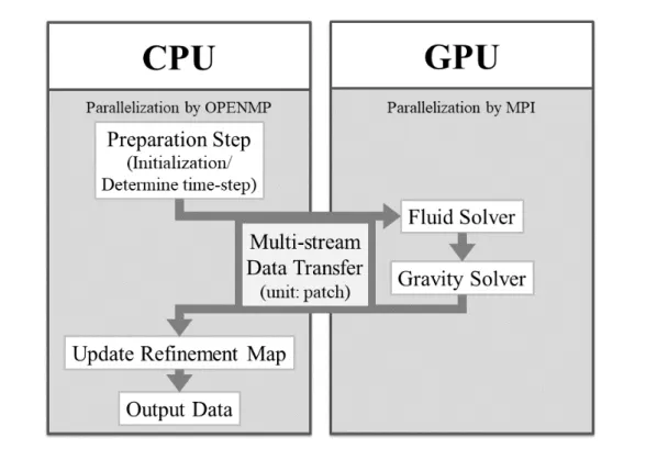
Figure 2.1 illustrates how GAMER evolve the system for a time-step. First, before solving the fluid equations, preparations such as determining the evolving time-step length are done by CPU. The data is then transfer to GPU patch by patch. A patch consists 8³

(29)

grid cells in our runs. After that, the patch data is evolved by numerically solving the fluid equations, and sent back to CPU for subsequent steps like updating the refinement map (chapter 2.2.2) and the data output. In addition, GAMER is also capable of parallel computing for multi-node clusters. OPENMP and MPI are applied for the parallelization of CPU and GPU, respectively.

Figure 2.1: CPU + GPU cooperation in GAMER

During the whole process, the required communication between CPU and GPU in- cludes the following three steps.

1. The downstream data transfer from CPU to GPU 2. Invoke GPU kernels to solve the fluid equations 3. The upstream data transfer from GPU back to CPU

In practice, there are multiple streams that each of them executes the above three steps for a specific number of patches. To further optimize the performance, the concurrent execution approach is implemented to reduce the communication time. For each stream, once it finish the downstream transfer (step 1) for the first bunch of data and proceeds to

(30)

the step 2, meanwhile it begins the step 1 for the second bunch of data. After that, the stream starts the step 3 for the first bunch of data, the step 2 for the second bunch of data, and the step 1 for the third bunch of the data simultaneously. Each stream can process at most three bunches of data concurrently, the code performance is thus further improved.

To sum up, the GPU acceleration is achieve by (1) proper workload distribution to CPU and GPU and (2) multi-stream data transfer with the concurrent execution.

2.2.2 Adaptive mesh refinement (AMR) technique

Another important feature of GAMER is the implement of the adaptive mesh refinement (AMR) technique. During the simulation, the local resolution may increase or decrease according to some specific refinement criteria. For example, if one wants to resolve a compact astrophysical structure, he may let the refinement depend on the local density value. The unrefined grid cells is defined as refinement level 0. Upon refinement, a level n patch is refined into 8 level n+1 patches. The local resolution increases by 2 in each dimension. In GAMER, according to the given refinement criteria, the refinement map is constructed initially and is updated every computational time-step. In GAMER, the system is evolved level by level, starting from the level 0. In order to improve the accuracy of coarse grid cells and retain the consistency across adjacent coarse and fine grid cells, the following two operations are carried out.

1. If there are fine grid cells inside a coarse grid, the physical quantities of the coarse grid is replaced by the corresponding spatial average of the fine grids.

2. Near the boundary between coarse and fine grids, correct the flux and the electric field to guarantee the mass conservation and zero magnetic field divergence across the boundary.

Again, as for the detailed strategy of AMR applied in GAMER, one can refer Schive et al. (2010).

(31)

2.3 Numerical scheme

We use the relaxing total variation diminishing (RTVD) scheme to solve the ideal MHD equations (Jin and Xin, 1995; Trac and Pen, 2003; Pen et al., 2003). In this scheme, each flux term in the fluid equations is formulated as the superposition of the leftward and the rightward flux. We take advantage of this feature to implement the essential barotropic equation of state. Meanwhile, with this scheme one can evolve the fluid system efficiently since less computational operations are required. However, it should also be noted that the scheme might not resolve all the particular structures compared to the complicated scheme that fully trace all the MHD characteristics.

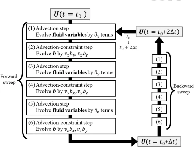
2.3.1 RTVD scheme

In the RTVD scheme, the fluid equations and the induction equation are solved sepa- rately. Moreover, the advection along the three directions (x, y, z) is also asynchronously evolved. Hence, to solve the MHD equations for a full time-step, six operations are ex- ecuted sequentially – (1) update the fluid variables along x-direction, (2) evolve the v_x- terms in the induction equation, (3) update the fluid variables along y-direction, (4) evolve the v_y-terms in the induction equation, (5) update the fluid variables along z-direction, and (6) evolve the v_z-terms in the induction equation. The sum of these six operations are called the forward sweep. After evolve a system for a time-step by the forward sweep, the backward sweep is executed to evolve the next time-step. The backward sweep consists the same six operations, but the executing order is reverse – (6)→ (5) → (4) → (3) → (2)

→ (1). After that, we use the forward-backward sweep combination to evolve the system further until the end of the run. Notice during the fluid update operations (1), (3), and (5) the magnetic variables are fixed, and the fluid variables are not evolving during the magnetic field update operations (2), (4), and (6). The flow chart of the RTVD scheme is summarized in figure 2.2.

(32)

Figure 2.2: Flow chart of the RTVD scheme

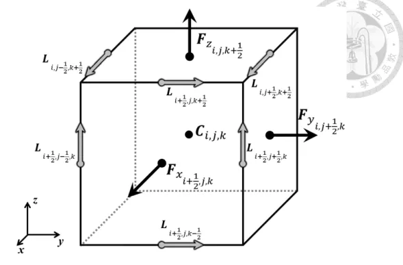
Meanwhile, the physical variables are categorized into three types according to their centering. They are

1. cell-centered variables (C) such as the fluid variables,

2. face-centered variables (F_x, F_y, F_z) such as the flux to evolve the fluid variables and the magnetic field, and

3. line-centered variables (L) such as the electric field in the induction equation to evolve the magnetic field.

The location of each type of the variable in a grid cell is illustrated in figure 2.3, along with the corresponding spatial indices. In addition, their characteristics are summarized in table 2.1.

(33)

Figure 2.3: Schematic picture of the variable centering

Location Symbol Indices Physical Variables

Cell-centered C (i, j, k) ρ, v, e, P

Face-centered

F_x (i± 1/2, j, k) b_x, x-direction fluid flux F_y (i, j± 1/2, k) b_y, y-direction fluid flux Fz (i, j, k± 1/2) bz, z-direction fluid flux Line-centered L

(i± 1/2, j ± 1/2, k)

Electric field (i± 1/2, j, k ± 1/2)

(i, j± 1/2, k ± 1/2)

Table 2.1: The centering of physical variables in the RTVD scheme

We now introduce the fluid update procedure in the RTVD scheme, as for and the magnetic field update, we leave it to chapter 2.3.2.

The fluid update in the RTVD scheme is dimensionally-split. We consider only the time and the spatial derivative terms of one direction in equation 2.3 at a time, namely solving the advection equation along a specific direction. As mentioned above, the flux terms are decomposed into two parts, that is,

F_RTVD=

(cU + F 2

)

−

(cU− F 2

)

, (2.8)

where the first and the second term represent the rightward and the leftward flux, respec-

(34)

tively. Take the x-direction advection case for an example, the rightward flux locates on the right face of a grid cell (Fx i+1/2,j,k in figure 2.3), while the leftward flux are on the center of the left face (F_{x i}_−1/2,j,kin figure 2.3). The outcome numerical flux F_RTVDacross the right face of a grid cell is then the superposition of the leftward flux of the neighbor cell in +x direction and the rightward flux of its own. Meanwhile, c is the flux freezing speed that should set to be the maximum information transfer speed in the system. In the case of the fluid update, c = |vi| +√

γP /ρ + b²/ρ, where v_i = v_x, v_y, v_z depending on the advection direction.

To ensure the second order accuracy in time, a second order Runge-Kutta method is applied for the advection step. The system is evolved by half a time-step with equation (2.8) first, and then the updated variables are evolved further to get the full time-step solution. During the second half step, the van Leer flux limiter is applied to guarantee that the total variation decreases over time.

2.3.2 Solving the induction equation

The magnetic field is updated by solving the induction equation 2.1d. The critical issue here is that the divergence free criterion of the magnetic field must not be violated during the evolution. In the following paragraphs, we introduce the advection-constraint step applied in the RTVD scheme to update the magnetic field, and show its capability to reduce the divergence error to the machine precision level.

In the induction equation, the spatial derivative of the electric field terms (−v × b in ideal MHD) are separately calculated according to their velocity direction. For example, after the fluid update step along x-direction is done in the forward sweep, we update b by the vxBy and vxBz terms. Here, we focus on the vxBy terms to illustrate the idea of the advection-constraint step. Similar arguments can easily apply to the other terms.











∂b_x

∂t = ∂

∂y(v_xb_y) ,

∂b_y

∂t =− ∂

∂x(v_xb_y) ,

(2.9)

(35)

We write down the term associated with v_xB_y in the induction equation as equation 2.9. The former equation has the form of the advection equation, and can be solved by the same method as mentioned in chapter 2.3.1. It should be noted that the electric field terms is line-centered since the magnetic field is face-centered. Another difference is that the flux freezing speed is adjusted to c = |vx|. Suggested by Pen et al. (2003), we used the spatially smoothed value of v_xto gain more stability.

After solving the advection equation in the magnetic field update step, we immediately use the newly calculated v_xB_y to solve the second equation of equation 2.9. The step is called the constraint step since it guarantees the system to obey the zero divergence constraint within the machine precision, provided the initial condition is divergence-free.

The proof is given in the following paragraphs.

Numerically, we consider the divergence of the magnetic field over a control volume, like a grid cell. Use the divergence theorem one has

∫

cell

∇ · bdτ =

∫

cell surface

b· ds = 0. (2.10)

Consider the magnetic field is face-centered and the cells are always cubic in GAMER, the above surface integral can be written as (Evans and Hawley, 1988)

( bx i+1

2,j,k− b_{x i}₋1 2,j,k

) +

( by i+,j1

2,k − b_{y i,j}₋1 2,k

) +

(

bz i,j,k+1 2

− b_{z i,j,k}₋1 2

)

= 0.

(2.11)

Equation 2.11 is the divergence free criterion numerically. Now, assume that the cri- terion is satisfied at time t. We calculate the divergence of the magnetic filed at the next time-step t + ∆t. Again we focus on the vxB_y terms first. Here the b(z) is not updated, so we write down the divergence of the magnetic field in x- and y- directions only. After

(36)

the evolution for a time-step, (

b^t+∆t

x i+1

2,j,k− b^t+∆t

x i−1 2,j,k

) +

( b^t+∆t

y i,j+1

2,k− b^t+∆t

y i,j−1 2,k

)

= (

b^t

x i+1

2,j,k− b^t

x i−1 2,j,k

) +

( b^t

y i,j+1 2,k− b^t

y i,j−1 2,k

)

− ∆t

∆h (

− (vxb_y)

i+1 2,j−1

2,k+ (v_xb_y)

i−1 2,j−1

2,k

)

+ ∆t

∆h (

− (vxb_y)

i+1 2,j+1

2,k + (v_xb_y)

i−1 2,j+1

2,k

)

− ∆t

∆h (

− (vxb_y)

i−1 2,j−1

2,k+ (v_xb_y)

i−1 2,j+1

2,k

)

+ ∆t

∆h (

− (vxb_y)

i+1 2,j−1

2,k + (v_xb_y)

i+1 2,j+1

2,k

)

. (2.12)

The last 4 terms on the RHS of equation 2.12 cancel out, so the system is still divergence free. Same proof can easily be written down for the other electric field terms in the induction equation. Therefore, we conclude that along with the advection step mentioned above, the advection-constraint step can evolve the magnetic field without generating any magnetic monopoles.

(37)

Chapter 3 Simulation setup

3.1 Initial and boundary conditions

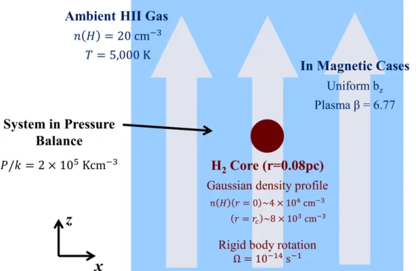
Figure 3.1: Initial conditions before the core relaxation

Initially, an isolated core located at the center of the computational domain. The den- sity profile is a Gaussian function with n(H)(r = 0)/n(H)(r = r_c) = 5, where r_c= 0.08 pc is the initial core radius. The core also exhibits a weak rigid body rotation along the z-axis with Ω = 10⁻¹⁴s⁻¹. The whole computation domain is at least 2.29³ pc. Outside the tiny core is the immense ambient HII gas with n(H) = 20 cm⁻³and T = 5,000 K. The

(38)

core and the ambient gas is in the pressure balance and throughout the domain there is a uniform magnetic field b along the z-axis. The schematic picture of the initial is shown as figure 3.1. As for all the boundaries, we choose periodic boundary conditions.

Core Center Core All Domain

Name n (H) T Mc Erot/Egrav Emag/Egrav B λ β ^a EOS

(cm⁻³) (K) (M_⊙) (%) (%) (µG)

M 4.32× 10⁴ 9.26 0.95 0.29 39.74 10.12 1.58 6.77 Type 1

M2 4.32× 10⁴ 9.26 0.95 0.29 39.74 10.12 1.58 6.77 Type 2

H 3.70× 10⁴ 10.81 0.81 0.34 0 0 ∞ ∞ Type 1

aPlasma β, β≡ 2p/b²

Table 3.1: Model characteristics before the core relaxation

Based on the above framework, we present 3 models with their characteristics listed in table 3.1. In model H, there is no magnetic present and the core mass is small. The magnetic cases, model M and model M2, only have difference in the equation of state, which is discussed in next section.

We let the core stably oscillate for tens of periods within the ambient gas. Until it is fully relaxed, we launch a Gaussian pulse toward the core. The setting of the pulse are illustrated in chapter 3.4.

3.2 Equation of state

Follow Zhang2015, consider the cosmic ray heating and the nonlinear cooling from molec- ular line emissions, we apply a special barotropic equation of state (EOS). In the approach, the pressure is modeled as

P = a (s) g (ρ)≡ a (s) ( ρ

ρ₀ )γ(ρ)

, (3.1)

where a(s) is the entropy function proportional to the entropy s. γ(ρ) is given by

γ (ρ) = γ0− ∆γ tanh



ln (ρ

ρ0

)

η



 . (3.2)

(39)

As listed in table 3.2, we apply two types of the equation of state differing in the rate of change in γ(ρ) with ρ, mainly for the transition region between the core and the ambient gas. The behavior of γ(ρ) is depicted as figure 3.2. Generally speaking, γ(ρ)∼ 0.7 for the core and the ambient γ(ρ)∼ 1.1 representing the near-isothermal gas. The soft equation of state models the efficient cooling inside the cold core.

Figure 3.2: The density dependence of γ(ρ) for the two types of the equation of state. Typ- ical hydrogen number density n(H) is 10⁴ cm⁻³for the core and 20 cm⁻³for the ambient gas.

EOS Type γ0 ∆γ ρ0(g cm⁻³) η Type 1 0.9 0.2 2.446× 10^{−21 a} 1.0 Type 2 0.9 0.2 2.446× 10⁻²¹ 2.0

aEquivalent to n(H) = 1473 cm⁻³

Table 3.2: Two types of the equation of state

From equation 3.1, the sound speed c_S is given by

c²_S = P ρ



γ − ∆γ η ln

( ρ ρ₀

) 1 − tanh²



ln (ρ

ρ0

)

η











 . (3.3)

(40)

As for the relation between the internal energy density e and the pressure p, we start from the first law of thermodynamics

de

ρ −e + P

ρ² dρ = 0, (3.4)

so that

e

P = ρ

g (ρ)

∫ _ρ

0

g (x)

x² dx. (3.5)

Define y≡ ln(ρ/ρ0). We approximate the integral on the RHS of 3.5. The results are

e p ∼











1

γ0+∆γ−1, y <−η,

(ρ ρ0

)ay+b[

e^{−η(aη−b)} γ0+∆γ−1

+¹₂√_π

ae^b2^4a(

erf (√

a(

y + _2a^b ))

− erf(√

a(

−η +_2a^b )))]

, −η ≤ y < η,

1 γ0−∆γ−1 +

(ρ ρ0

)aη+b[

e^{−η(aη−b)}

γ0+∆γ−1 − _γ^e^−η(aη+b)₀_−∆γ−1 +¹₂√_π

ae^b2^4a(

erf (√

a(

η + _2a^b ))

− erf(√

a(

−η +_2a^b )))]

, y≥ η, (3.6) where a≡ ∆γ/η, b ≡ 1 − γ0. In practical, equation 3.6 is applied to get the pressure from the given e to calculate the fluxes that updates the fluid variables.

(41)

3.3 Mesh refinement criteria

In all the presented runs, a patch is adaptively refined by its distance to the core center and the maximum density value within. A patch is refined to level n when the distance to the core center is smaller than∼ 2⁴⁻ⁿr_cwith the maximum refinement level n = 3. At the same time, if the maximum density within a patch exceeds n(H) = 3375× 4ⁿ⁻¹cm⁻³, the grids are refined to level n with the maximum refinement level n = 7. With the aid of the AMR technique, we efficiently resolve the immense ambient gas and the dense core simultaneously.

3.4 The Gaussian fast pulse

After a long period of relaxation, we launch a pulse toward the fully-relaxed core. The definition of full relaxation is that the maximum density within a core at its maximum contraction phase is only≤ 10% larger relative to the average value over a core oscillat- ing period T₀. As for the pulse locating at (X_GP, Y_GP, Z_GP), its density perturbation is characterized by a Gaussian function with the width σ. Moreover, we treat the pulse as the resultant wave packet from the superposition of fast magneto-sonic waves of various frequency. The Gaussian wave pulse can then be formulated as the following form, where θ is the angle between the pulse propagating direction k and the z-axis. Note that the sound speed c_Sand the Alfv´en speed c_A≡√

b²/ρ in this section refer to the corresponding value in the ambient gas.

δρ = δρ_ge

−(^{sin θ}⁽^x^−XGP⁾^{+cos θ}⁽^z^−ZGP⁾²)

2σ2 , δP = c²_Sδρ,

δv_x = ^k_ω (

1− _ω^k²2c²_A )₋₁

c²_Ssin θ^δρ_ρ

0, δb_x =−_ω^kc_A√

ρ₀cos θδv_x,

δv_y = 0, δb_y = 0,

δvz = _ω^kc²_Scos θ_ρ^δρ

0, δbz = _ω^kcA√

ρ0sin θδvx,

(3.7)

(42)

The phase speed c_F is given by

cF ≡ ω k =

√1

2(c²_A+ c²_S) + 1 2

√

(c²_A+ c²_S)²− 4c²_Ac²_Scos²θ. (3.8)

Since the pulse has wave-like nature, we define the characteristic wavelength of a Gaussian fast pulse to be 4σ, so that the pulse characteristic frequency ν ≡ cF/4σ. Mean- while, the characteristic frequency of the oscillating core ν₀is defined as 1/T₀. The ratio of the characteristic frequencies ν/ν₀ relates the wave-like pulse to the periodically oscillating core, and is considered to be the ideal parameter to research the interaction between the core and the pulse.

Table 3.3 describes the characteristics of the pulses to launch. In model PM90 and model PM0, the pulses are launches toward the fully-relaxed core in model M, while in model PH the target is the fully-relaxed core in model H. Model PM90 and PM0 differs in the incident direction of the pulse.

Ambient Gas Name Initial Condition Configuration Core Oscillating Period c_S c_A

(Myr) (kms⁻¹) (kms⁻¹) PM90 Relaxed model M k⊥ binit ∥ Ωinit a 0.61 9.57 4.95

PM0 Relaxed model M k∥ binit ∥ Ωinit 0.61 9.57 4.95

PH Relaxed model H k⊥ Ωinit 0.67 9.57 0

aThe subscript init refer to the stage before the core relaxation

Table 3.3: Gaussian fast pulse characteristics

The pulse in model PM90 has the following form.

δρ = δρ_ge⁻⁽

x−XGP)²

2σ2 , δP = c²_Sδρ, δvx =√

c²_A+ c²_S^δρ_ρ

0, δbx = 0,

δv_z = 0, δb_z = √^c^Aρ0δρ,

(3.9)

c_F =

√

c²_A+ c²_S. (3.10)

(43)

As for the pulse in model PM0,

z−ZGP)²

2σ2 , δP = c²_Sδρ,

δv_x = 0, δb_x = 0,

δv_z = c_S^δρ_ρ

0, δb_z = 0,

(3.11)

c_F = c_S. (3.12)

Finally, the pulse in model PH can be characterized by

x−XGP)²

2σ2 , δP = c²_Sδρ, δv_x = c_S^δρ_ρ

0, δb_x = 0,

δv_z = 0, δb_z = 0,

(3.13)

c_F = c_S. (3.14)

(44)

(45)

Chapter 4 Results

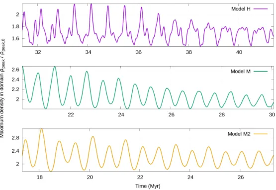
4.1 Core relaxation

Figure 4.1: Peak density evolution of the relaxing cores. The peak density has been normalized to the initial value for each model.

Starting from the initial conditions described in chapter 3.1, in all the three models, the core does not spontaneously collapse. Instead, after the first few vigorous oscillations, the contraction and the expansion of the core gradually becomes milder and milder. Define