Proceedings of 7th PAAMES and AMEC2016 13-14 Oct., 2016, Hong Kong
Evaluation of the Speed Loss in Seaway by Computational Methods
Chun-Ta Lin
1, Ching-Yeh Hsin
1, Ling Lu
1, Chi-Chuan Chen
2, and Cheng-Wen Lin
2
1Department of Systems Engineering and Naval Architecture, National Taiwan Ocean University, Keelung, Taiwan
2CR Classification Society, Taipei, Taiwan
Abstract
In this paper, the speed loss in seaway is evaluated by simulating the self-propulsion test in calm water and in sea state. The weather factor thus can be computed from ship speeds obtained at the same power in both calm water and waves. In the presented method, we use both the potential flow method and the viscous flow method. Two different approaches for evaluating the speed loss in sea way are presented. For the first approach, “Double-body model” is used in the viscous flow computations to compute the viscous drag, and both wave-making resistance and added resistance are computed by potential flow methods. For the second approach, the free surface effects are included in the viscous flow computations. Therefore, ship hull forces in calm water are all computed by the viscous flow method. The added resistance is still computed by a potential flow method. The body force method is used to represent the propeller effects in all approaches. The KCS model ship is used to demonstrate the speed loss computations, and results from two approaches are compared to each other and investigated.
Keywords: Body force method, self-propulsion simulation, EEDI, ship speed loss, weather factor, propeller in waves
1 Introduction
The fuel efficiency in seaway becomes more important due to environmental regulations, and the speed loss in seaway is quantitatively evaluated by weather factor in EEDI (Energy Efficiency Design Index).To compute the speed loss, the ship hull resistances in both calm water and waves have to be computed. Then the ship speeds in different sea states can be evaluated based on the propeller performance in waves. In this paper, we will divide the wave effects into two factors. The first one is the effect due to ship positions in motion and the induced velocity due to waves, and the second one is the interactions between the ship hull and the propeller. In this paper, these two factors are assumed to be
independent to each other. Instead of using the viscous flow RANS method to directly simulate the whole physical phenomena, we will use both the potential flow method and the viscous flow method. Since the viscous effects are less important in ship motion problems, to use the potential flow method is appropriate. On the other hand, the interactions between the ship wake and the propeller are dominated by the viscous effect, thus the viscous flow RANS method is used. The body force method (Kerwin et al., 1994; Hsin et al., 2000, 2008; Wei, 2012) is used to represent the propeller effects, and the reason is not only because the simplicity, but also because we can separate the flow field into
“propeller inflow” and “propeller induced velocity” by using this method. The inflow due
to the propeller-hull interaction can be added to the inflow due to the ship motions and wave induced velocities, and become the “total inflow” of a propeller in waves.
The propeller performance in waves has been studied by many researchers. Journée (1976) applied an approximate method to study the ship motion effects to the propeller performance, and he has also carried out experiments to make the comparison. Faltinsen (1980) has investigated the resistance and propulsion in seaway, and he claims that since the encounter frequency of the incoming wave is far smaller than the propeller rotational frequency, only the vertical velocities due to motions are critical to the propeller performance in waves. The variation of the propulsion thrust in wave can be computed by quasi-steady flow method, that is, to solve the thrusts at different time step, and the thrust in waves will be the mean value of these. Nakatake et al. (1986) later developed a panel method using source and sink distributions to simulate the ship hull, propeller and rudder, and studied the interactions of hull/propeller/rudder by computations. Ando et al. (1989, 1990) have verified the above computations by experiments.
Recently, Kashiwagi et al. (2004) investigated the propeller performance in waves by using the Enhanced Unified Theory (EUT), which is derived from ship motion theory. Chuang and Steen (2011) have studied the power and speed loss in waves by experiments.
2 Bare hull resistance
The bare hull resistance computation is first demonstrated here, and the model scale of KCS ship (1:31.599) is used for the computation. The commercial software STAR-CCM+ is used for RANS computations, and Fig. 1 shows the boundary conditions set in the computations.
Noted that the free surface effect is included when activating the free surface boundary condition. Fig. 2 shows the grid arrangement of the ship hull when considering the free surface effect, and around 4.5 million grids are used.
The SST k-ω model is selected as the turbulence model. We first validate the computational results of the bare hull, and the computational error is only 0.25%. Where the computed resistance is 81.0, and the experimental data is 80.8. Fig. 3 shows the comparison of the computational results and experimental data of the ship wake on the propeller plane, and Fig. 4 shows the comparison of the wave profiles
between the computational results and experimental data. Both the force and flow field from computations are within acceptable accuracy.
Fig. 1: The boundary conditions set for the self-propulsion simulation, and the free surface boundary condition is activated.
Fig. 2: The grid arrangement of the KCS ship hull when considering the free surface effect.
Fig. 3: The comparison of the computational results (color lines) and experimental data (black lines) of the ship wake on the propeller plane.
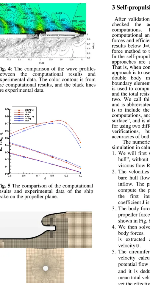
Fig. 4: The comparison of the wave profiles between the computational results and experimental data. The color contour is from the computational results, and the black lines are experimental data.
Fig. 5 The comparison of the computational results and experimental data of the ship wake on the propeller plane.
Fig. 6 The grid arrangement for the body force disk.
3 Self-propulsion simulations
After validations of the bare hull results, we checked the accuracy of propeller force computations. Fig. 5 shows both the computational and experimental KCS propeller forces and efficiency. The error is within 5% for results below J=0.9. We then applied the body force method to the self-propulsion simulations.
In the self-propulsion simulations, two different approaches are used for verification purpose.
That is, when computing the hull resistance, one approach is to use the RANS method to compute double body model, and a potential flow boundary element wave-making resistance code is used to compute the wave-making resistance, and the total resistance is the summation of these two. We call this approach as “double body”, and is abbreviated to “DB”. The other approach is to include the free surface effect in RANS computations, and we call this approach as “free surface”, and is abbreviated as “FS”. The reason for using two different approaches is not only for verifications, but also to investigate the accuracies of both approaches.
The numerical procedure of self-propulsion simulation in calm water is described as follows:
1. We will first solve the flow field of a “bare hull”, without the propeller in operation. The viscous flow RANS method is used here.
2. The velocities at the propeller plane for the bare hull flow are retrieved as the propeller inflow. The propeller BEM is then used to compute the propeller flow and forces. For the first iteration, an initial advanced coefficient J is given.
3. The body forces are then computed from the propeller forces, and put in the RANS grid as shown in Fig. 6.
4. We then solve the ship flow again with the body forces. The flow at the propeller plane is extracted again, and this is the total velocityU.
5. The circumferential mean propeller induced velocity calculated in the last iteration by potential flow BEM method is denoted byUP, and it is deducted from the circumferential mean total velocity (U) calculated in step 4 to get the effective inflow UE.
E P
U = U - U (1)
6. UEis then used as the propeller inflow in the propeller BEM to compute the propeller flow and forces again.
7. We then repeat steps 5 and 6 until the solution is converged. Both the hull resistance RT and propeller thrust T can be obtained, and the self-propulsion point is reached when equation (2) is satisfied.
T SFC
TR F (2) In equation (2), FSFC is the skin friction correction to correct the scale effect.
8. If equation (2) is not satisfied, the Newton method is used to get a new advanced coefficient for the propeller. The iteration goes back to 2. until equation (2) is satisfied, and the self-propulsion point is obtained.
The above numerical procedure is used to compute the self-propulsion point of KCS model ship in calm water, and Table 1 shows the comparison of numerical results and experimental data. One can see most of the computational results are within 5% error, and
“free surface” (FS) approach gives a better prediction.
Table 1. The comparison of numerical results and experimental data.
1- n
(rps)
EXP 0.792 9.5 0.1700 0.2880
DB 0.774 0.734 9.27 0.1658 0.2745 Err(%) -2.27 -2.42 -2.47 -4.69
FS 0.793 0.739 9.42 0.1629 0.2710 Err(%) 0.13 -0.84 -4.18 -5.90
1-t D H R O
EXP 0.853 0.743 1.077 1.011 0.682 DB 0.873 0.805 1.128 1.001 0.713 Err(%) 2.34 8.34 4.74 -0.99 4.54
FS 0.864 0.781 1.090 1.001 0.7153 Err(%) 1.29 5.11 1.21 -0.99 4.88
Once the numerical procedure for simulating the self-propulsion in calm water is established, it can be extended to simulate the self- propulsion in sea states. Since the circumferential mean propeller forces are used, the time mean wave added resistance is used for self-propulsion simulations in sea states. The strip theory is used for calculating the wave added resistance in this paper. The numerical procedure to simulate the self-propulsion in sea states is the same as in calm water except
equation (2) is modified as the following equation.
T WAVE SFC
TR R F (3) In equation (3), RWAVE is the wave added resistance. The speed loss thus can be obtained from the self-propulsion simulations in calm water and in sea states. The full scale KCS ship is used for demonstrations.
In Table 1 and the following tables, the nomenclature is listed as follows:
we: The effective wake fraction
JA: Advance coefficient
TB, QB
K K : Thrust coefficient and torque coefficient behind the hull
t: Thrust deduction factor
D: Quasi-propulsive efficiency = O H R
H: Hull efficiency = 1t/1w
R: Relative rotative efficiency = B/ O
B: Behind hull efficiency = O R
O: Open water efficiency
P: Propulsive efficiency = O H R S G
S: Shafting efficiency
G: Gearing efficiency
RT: Total resistance
T: Propeller thrust
EHPPE: Effective horsepower = R VT
BHPPB: Brake horsepower
Also the subscript “s” denotes full scale results.
The speed loss here is defined as the difference between obtainable ship speeds at the same given power in calm water and in sea states. In order to obtain the speed loss, the ship power curves are constructed by self-propulsion simulations at three different ship speeds, and the speed difference thus can be obtained from power curves in calm water and in sea states.
Since IMO rule use Beaufort 6 condition, the equivalent Sea State 5 condition is used here.
Table 2 shows the computational results of the self-propulsion simulation in calm water using
“double body” approach, and Table 3 shows the computational results of the self-propulsion simulation in calm water using “free surface”
approach. Similarly, Table 4 and Table 5 show the computational results of the self-propulsion simulations in Sea State 5 using two different approaches.
Table 2. The computational results of the self- propulsion simulation in calm water using
“double body” approach.
1- 1- KT/J2
16 0.786 0.868 0.274 0.757
20 0.792 0.870 0.266 0.761
24 0.798 0.872 0.285 0.750
16 0.682 1.151 1.001 0.809
20 0.717 1.140 1.000 0.802
24 0.715 1.129 1.001 0.792
(N) EHP BHP
16 618918 713039 6931 8572
20 955543 1098325 13376 16683 24 1498198 1718117 25167 31779
Table 3. The computational results of the self- propulsion simulation in calm water using “free surface” approach.
1- 1- KT/J2
16 0.795 0.872 0.287 0.749
20 0.800 0.869 0.271 0.758
24 0.808 0.865 0.298 0.743
16 0.713 1.138 1.002 0.797
20 0.718 1.118 1.001 0.787
24 0.714 1.088 1.000 0.762
(N) EHP BHP
16 665776 763504 7455 9359
20 992932 1142614 13899 17665 24 1594869 1843779 26790 35178
Table 4. The computational results of the self- propulsion simulation in sea state 5 using
“double body” approach.
1- 1- KT/J2
16 0.804 0.881 0.026 0.673
20 0.805 0.875 0.024 0.694
24 0.809 0.877 0.024 0.695
16 0.689 1.136 1.003 0.769
20 0.699 1.119 1.062 0.813
24 0.699 1.114 1.003 0.765
(N) EHP BHP
16 97166 110291 10663 13868
20 137773 157455 18900 23247 24 200333 228430 32979 43116
Table 5. The computational results of the self- propulsion simulation in sea state 5 using “free surface” approach.
1- 1- KT/J2
16 0.808 0.872 0.027 0.666
20 0.813 0.877 0.024 0.694
24 0.818 0.872 0.024 0.694
16 0.690 1.105 1.002 0.749
20 0.699 1.101 1.003 0.757
24 0.699 1.079 1.002 0.741
(N) EHP BHP
16 101992 116963 11193 14953 20 141588 161446 19423 25666 24 210197 241052 34603 46721
Fig. 7: The power curves in calm water and in sea state 5 computed from two different approaches.
4 Speed loss
All the above self-propulsion results are then represented by power curves, and they are shown in Fig. 7. In Fig. 7, both power curves in calm water and in Sea State 5 computed from two approaches are shown, and one can see the differences of Brake Horsepower (BHP) predicted by two different approaches. We can then obtain the speed loss at a given BHP, and the speed loss at BHP=20,000 and at BHP=30,000 are demonstrated in Fig. 7 and Table 6. For example, the speed loss is 2.0 knots at BHP=30,000, and the ratio of two speed is 0.913. In Table 6, fw is similar to the “weather
factor” in EEDI and we use this to represent the speed ratio at Sea State 5 and in calm water.
Table 6 shows that the larger the BHP, the less the speed loss. Also, the “free surface”
approach predicts a larger speed loss, and the differences between two approaches are very small for BHP=30,000, but relatively large for BHP=20,000. This is because the difference between the computational results of wave- making resistance is larger at lower BHP.
Table 6. The computational results of speed loss
Model State 20000 PS 30000PS
Double Body
Calm Water 21.034 kts. 23.588 kts.
Sea State 5 18.736 kts. 21.606 kts.
Speed Loss -2.30 kts. -1.98 kts.
fw 0.891 0.916
Free Surface
Calm Water 20.675 kts. 22.994 kts.
Sea State 5 18.024 kts. 20.991 kts.
Speed Loss -2.65 kts. -2.00 kts.
fw 0.872 0.913
Diff. Speed Loss 13.3% 1.0%
fw -2.2% -0.4%
5 Conclusions
In this paper, both the potential flow and viscous flow computational methods are used for the evaluation of speed loss. Two different approaches are presented, and they are “double- body model” and “free surface model”.
Computational examples is shown in the paper, and results show that the presented method can be successfully applied to the speed loss computations. This means not only that the body force method can be successfully used to simulate the propeller/hull interactions, but also the numerical procedure of self-propulsion simulations presented in the paper is applicable.
In the presented work, we have established a method to integrate ship motion computational method, the propeller boundary element method, and the viscous flow RANS method to evaluate the speed loss and weather factor in EEDI.
Acknowledgements
The authors would like to express their gratitude to CR Classification Society, Taipei for their funding support.
References
Ando, J., Kataoka, K., and Nakatake, K., "Free Surface Effect on the Propulsive Performance of a Ship (2nd Report)", West Japan Soc. Nav.
Arch. Trans. (77), pp. 9-28, March, 1989
Ando, J., Shiota, H., Kataoka, K., and Nakatake, K., "Free Surface Effect on the Propulsive Performance of a Ship (3rd Report)", West Japan Soc. Nav. Arch. Trans. (79), pp. 13-20, March, 1990
Chuang, Z. and Steen, S., "Prediction of Speed Loss of a Ship in Waves", Second International Symposium on Marine Propulsors (smp'11), Hamburg, Germany, June 2011
Faltinsen, O.M., "Prediction of Resistance and Propulsion of a Ship in a Seaway", Proc. 13th Symposium on Naval Hydrodynamics, 1980, Tokyo, Japan
Hsin, C. Y., Tzeng, I. W., and Chang, C. Y.,
“Propeller Analysis and Design Using a Coupled Viscous/Potential Flow Method”, Proceedings of the 4th International Conference on Hydrodynamics, Yokohama, Japan, September, 2000
Hsin, C.Y., Chang, S.F., Chang, F.N. and Chou, S.K., “The Design of an Energy-Saving Rudder by Computational Methods”, Proceedings of the 8th International Conference on Hydrodynamics (ICHD2008), Nantes, France, 2008
Journée, J.M.J., "Prediction of Speed and Behaviour of a Ship in a Seaway", Report 0427-P, 1976, Delft University of Technology, Ship Hydromechanics Laboratory, Delft,The Netherlands
Kashiwagi,M., Sugimoto, K., Ueda, T., Yamasaki, K., Arihama, K., Kimura, K., Yamashita, R., Itoh, A. and Mizokami, S., "An Analysis System for Propulsive Performance in Waves", Journal of the Kansai society of naval architects, No. 241, 2004
Kerwin, J.E., Keenan, D.P, Black, S.D.B., “A coupled viscous /potential flow design method for wake-adapted, multi-stage, ducted propulsors using generalized geometry”, SNAME Transactions, 102, pp.23-56, 1994 Nakatake, K., Oda, K., Kataoka, K., Nishimoto,
H. and Ando, J., "Free Surface Effect on the Propulsive Performance of a Ship (1st Report)", West Japan Soc. Nav. Arch. Trans. (72), August, 1986, pp.129-139
Wei, W.-C., “The Influence of the Propeller Loading Distributions to the Propulsive Efficiency”, Master thesis, Nation Taiwan Ocean University, 2012