FAT-based adaptive control for flexible-joint robots without computation of the regressor matrix

2006 IEEE International Conference on Systems, Man, and Cybernetics

October 8-11, 2006, Taipei, Taiwan

FAT-based Adaptive Control for Flexible-joint Robots without Computation of the Regressor Matrix

Ming-Chih Chien and An-Chyau Huang, Member, IEEE

Abstract-An adaptive controller is presented in this paper to control an n-link flexible-joint manipulator with time-varying uncertainties. The function approximation technique (FAT) is utilized to represent time-varying uncertainties in some finite combinations of orthogonal basis. The tedious computation of the regressor matrix needed in traditional adaptive control is avoided in the new design, and the controller does not require the variation bounds of time-varying uncertainties needed in traditional robust control. In addition, the joint acceleration is not needed in the controller realization. Via the Lyapunov-like stability theory, adaptive update laws are derived to give convergence of the output tracking error. A 2 DOF planar manipulator with flexible joints is used in the computer simulation to verify the effectiveness of the proposed controller.

I. INTRODUCTION

In practical applications, most controllers for robot manipulators equipped with harmonic devices are based on rigid-body dynamics formulation. To achieve high precision tracking performance, the joint flexibility should be carefully considered[1]. However, the modeling offlexible-joint robots is far more complex than that of rigid-joint robots. Besides, the mathematical model of the robot inevitably contains model inaccuracies such as parametric uncertainties, and unmodeled dynamics. Since these inaccuracies may degrade the performance of the closed-loop system, any practical design should consider their effects. Under the problems of joint flexibility and model inaccuracies, several strategies based on adaptive control or robust control for flexible-joint robots had been proposed.

Spong[2], [3] proposed an adaptive controller for flexible-joint robots by using the singular perturbation formulation. Chen and Fu[4] presented a two-stage adaptive control scheme for a single-link robot based on a simplified dynamic model. Khorasani[5] designed an adaptive controller using the concept of integral manifolds for n-link flexible-joint robots. Without using the velocity measurements, Lim et. al.[6] proposed an adaptive integrator backstepping scheme for rigid-link flexible-joint robots.

Dixon et. al.[7] designed an adaptive partial state feedback controller by using a nonlinear link velocity filter. Yim[8]

suggested an output feedback adaptive controller based on the backstepping design. Kozlowski and Sauer[9], [10] suggested

Ming-Chih Chien is with the Department of Mechanical Engineering, National Taiwan University of Science and Technology, 43, Keelung Road, Sec. 4, Taipei, Taiwan, ROC(e-mail: [email protected]).

An-Chyau Huang is with the Department of Mechanical Engineering, National Taiwan University of Science and Technology, 43, Keelung Road, Sec. 4, Taipei, Taiwan, ROC (Tel: +886-2-273-76490; Fax:

+886-2-273-76460, e-mail: achuang(mail.ntust.edu.tw).

an adaptive controller under the assumption of bounded disturbances to have semiglobal convergence. However, like most adaptive control strategies, the uncertainties should be linearly parameterizable with unknown constant parameters.

At the same time, some approaches based on robust control for flexible-joint robots had been proposed. Han and Chen[11] presented a robust composite control law for flexible-joint robot based on singular perturbation techniques.

Tian and Goldenberg[12] proposed a robust adaptive controller with joint torque feedback. Jain and Khorrami[ 13]

suggested a robust adaptive control for a class of flexible-joint robots that are transformable to a special strict feedback form.

Huang and Chen[14] proposed an adaptive backstepping-like controller based on FAT[15]-[21] for single-link flexible-joint robots with mismatched uncertainties. Similar to most backstepping design, the derivation is too complex to robots with more joints. In this paper, we would like to propose a FAT based adaptive controller for n-link flexible-joint robots without computation of the regressor matrix. The control strategy does not need to feedback joint acceleration. Convergence of the output error and the boundedness of all signals are proved with consideration of the effect of approximation error.

This paper is organized as follows: in section 2, we derive the proposed adaptive controller in detail; section 3 presents simulation results of a 2-D flexible-joint robot using the proposed controller; finally, some conclusions are given in section 4.

II. MAIN RESULTS

The dynamics of an n-rigid link flexible-joint robot can be described by[22]

D(q)q + C(q, q)q + g(q) ⁼ K( ^- q) O (1)

JO+BO+K(O-q) ⁼ u (2)

where qe 9i' is the vector of link angles, 0 ⁽ 91n is the vector of actuator angles, u E 9Vn is the vector of actuator

input torques, D(q) is the n x n inertia matrix, C(q, q)q is an n-vector of centrifugal and Coriolis forces, and g(q) is the gravity vector. J, B and K are n x n constant diagonal

matrices of actuator inertias, damping and joint stiffness, respectively. Here, we would like to consider the case when the precise forms of D(q) , C(q, q)q and g(q) are not

available and their variation bounds ^are not given. ^This

implies that traditional adaptive control and robust control

cannot be applicable. In the following, we would like to use the function approximation technique to design an adaptive controller for the flexible-joint robot. Moreover, it is well-known that derivation of the regressor matrix for the adaptive control of high DOF rigid robot is generally tedious.

For the flexible-joint robot in (1) and (2), its dynamics is much more complex than that of its rigid-joint counterpart.

Therefore, the computation of the regressor matrix becomes extremely difficult. Different form the conventional adaptive control schemes for robot manipulators, the proposed FAT-based adaptive controller does not need the computation of the regressor matrix. This largely simplifies the implementation of the control loop.

Define ^T = K(0 - q) to be the vector of transmission torques, so (1) arid (2) becomes[12]

D(q)q ⁺ C(q, q)q ⁺ g(q) ^{= T} (3)

J tT+B t+ T

^-

U-q(q,q) (4)

where J =JK- , B, =BK-1 and q(q,q)4= Jq +Bq.

Define signal vector s = e + Ae and v = d - Ae, whereq d E in is the vector of desired states, e = q d-q ^is

the state error, and A = diag(2, 22,..., An) with Ai ^> 0 for all i 1, ... n. Rewrite (3) in the form

Ds+Cs+g+Dv+Cv= T (5)

A. Controller Design for Known Robot

Suppose D(q), C(q,q)q and g(q) are known, and we may design a proper control law such that T follows the trajectory below

T= g + Dv + Cv -PdS (6)

where Pd is a positive definite matrix. Substituting (6) into (5), the closed loop dynamics becomes Ds+Cs+ Pds = 0.

Define a Lyapunov function candidate as V = -s Ds. Its 2

time derivative along the trajectory of the closed loop dynamics can be computed as V = -s Tpds+T(D- 2C)s.

Since D-2C can be proved to be skew-symmetric, the above equation becomes V = -sTPds ^< 0. It is easy to prove that s is uniformly bounded and square integrable, and s is also uniformly bounded. Hence, s ^-- 0 as t -* oo, or we may say e -> 0 as t -X ^-. To make the actual T converge to the perfect T in (6), let us consider the reference model

JrTr +BrTr +KrTr= KrTd +Br+d +JrTd (7) where Tr E 9in is the state vector of the reference model and

T EdS ^{is the desired} states. Matrices Jr E 9Ixn Br ^E 9 nlXn and Kr ^E 91 fnXn are selected such that Tr -Td exponentially. Define Td(Td,d) ⁼ Kr(K;'BrTd +K'JrTd)

^I

^we

may rewrite (4) and (7) in the state space form as

(8) (9) mp = Apxp +Bpum-(Bpq

*. AXN +B.(Td +Td)

where xp =L [ ]T E 2n and Xm ⁼ [ITr ^Tr]T

^r

^{2n are}

augmented state vectors. AP = - n> ]e92nx2n and An1=LJ-1K 9J-Bj]ti ^{2nx2n are augmented}

system matrices. BP ^{= K] 2c n and}

Bm = K r ] E 2Xnx ^are augmented input gain matrices,

and the pair (Am,Bm) ^is controllable. Since all system parameters are assumed to be available at the present stage, we may select a controller in the form

U = Oxp +rd +h(Td,) (1 0)

where GC 91nx2n and qDEI91 x" satisfy AP +1BP = Am and B ^p =Bm , respectively, and hd(Td, q) = ¢TVd + q Substituting (10) into (8) and after some rearrangements, we may have the system dynamics

xp =AmXp+Bm(Td+Td) (11)

Define em = Xp - Xm and we may have the error dynamics directly from (9) and (11)

em = Ame. (12)

Let el = T- Tr be the output vector of the error dynamics (12) as

eC = Cmem (13)

where Cm E 9 nx2n is the augmented output matrix such that the pair (Am,Cm) is observable and the transfer function Cm(si-Am) 1Bm ^{is strictly} positive real. Since Am is stable, (12) implies em -* 0 as t ^{- oo .} This further gives

T -* Td as t -> -.

In summary, if all parameters in the n-rigid link flexible-joint robot (1) and (2) are available, the controller (10) can give asymptotic convergence tracking performance.

B. Controller Design for Uncertain Robot

Suppose D(q), C(q, q)qc ^and g(q) are not available, and q is not easy to measure, we would like to design a desired transmission torque Td so that a proper controller u can be constructed to have ^T -> Td . Instead of (6), let us design a desired transmission torque Td as

Td =g+Dv+Cv-Pds (14)

where Pd > nInXn, and D , C and g are estimates of

D(q), C(q,q) and g(q), respectively. Substituting (14) into (5), we may have the closed loop dynamics

Ds+Cs+Pds=(T-Td) (15)

+ (D - D)v + (C - C)v + (g - g).

If a proper controller u and update laws for D, C and g can

be designed, we may have Tr->Td, D ^- D, C -> C and g ^- g so that (15) can give desired performance. Let us consider the control law

u=OXP +'Id ^+h (16)

where h is an estimate of h. Substituting (16) into (8), we

may have the system dynamics

Xp =AmXp +Bm(Td + d)+Bp(I-h) (17)

Together with (9), we may have the error dynamics

m =Amem +Bp(h-h) (18)

eT Cmem (19)

Ifwe may design an appropriate update law such that h -4 h, then (18) implies em 0 as t -4

^-

. This further implies

T -> Td as t ^-- oo. Since D, C, ^g and h are functions of time, traditional adaptive controllers are not directly applicable. To design the update laws, let us apply the function approximation representation[ 15-21]

D=WDZD T +D (20a)

C=WTZc+ ^c (20b)

g=WTZg +£g (20c)

h = Wh Zh + (20d)

where WD C 91n 'Xn W E E / , Wg and

Wh e 9iflJxf are weighting matrices, 4 e Xn

E

Zg 9/gXl and Zh

^x

Zxl are matrices of basis functions, and t( ) are approximation error matrices.

The number ,89 represents the number of basis functions used. Using the same set of basis functions, the corresponding estimates can also be represented as

A^

Tr

D = WDZD (20e)

A

T

C = Wc Zc (20f

g =W Tz (20g)

h=WhZh T (20h)

Define W() = W(.) - W(.) , then equation (15) and (18) becomes

DS+CS+PdS=((T Td)

1T T T (21)

+WDZDV+VWCTZCV+Wg ^{Zg +}

²

where El =E1(D9ECIEg,S,4d) and £2 =F2(@h,em) are

lumped approximation errors. Since W() are constant vectors, their update laws can be easily found by proper selection of the Lyapunov-like function. Let us consider a candidate

~~ ~ ~~ ~~T1

V(s, em, WD, WC, Wg, W,h) ^{=-S DS+e} Ptem

Irrg ^{2 ml rn} (23)

1 ~ T ~~,

+-Tr(WDQDWD ₂ ⁺ WcQCWC ⁺ WgQgWg ⁺ Wh QhWh)

where Pt ⁼ pT e 2nx2n is a positive definite matrix

satisfying the Lyapunov equation

AmPt + PtAm =CM. ^The matrices QD

^I

QC ^(- v2&3xn

²

Qg ^e 91n/,gxn ^{Q9 and Qh E} 9tn', xnA, are

positive definite. The notation Tr(.) denotes the trace operation of matrices. The time derivative of V along the trajectory of (21) and (22) can be computed as

T T T

V=s Ds+-s Ds+e Pt em Pe

2 Mm Mm

+ Tr(WQDWD ⁺ WQCWC ⁺ Wg QgWg ^{+ W[} QhWh)

--s PS+ST e, -eTe +S TE ^+e T2

+r

*T T T T T

+ WT(ZDVST + QDWD) + W (Zcvs + QCWC) (24) +T{ W (ZgST ⁺ QgWg) + WI (ZhemPtBP + QhWh)]

According to the Kaman-Yakubovic Lemma, we have

PtB = CT by picking Bm = B . According to (24), the update laws can be selected as

WD =-QD ZDVS (25a)

WC= -Q -c'vsT (25b)

Wg Q-I ^{ZST (25c)}

(25d)

Wh =-Qh Zhe,

then (24) becomes

V =- ST e + eT ][£E (26)

where Q ⁼ x2] is positive definite due to I nxn Inxn

the selection Pd ^{> '} Inxn . Owing to the existence of £ and

SC2, ^the definiteness of ^V cannot be determined. Let us

proceed by representing (26) in the form

'~min

Q

If we select suitable Q and ^a proper set of basis functions,

Cm =Amm +BpWTZh +Bpi2 (22)

then V < 0 whenever [es] E{l6IkrII>Aij(Q) I1E2 ^>

This further concludes that ^el and s are uniformly ultimately bounded. To implement the desired transmission torque (14), the actuator input (16) and update law (25), ^we do not need the regressor matrix or the knowledge ofjoint accelerations.

The convergence of the parameters, however, ^can be proved to depend on the persistent excitation condition of the input.

Remark ^1. If the number of basis functions 8(.) is chosen to be sufficiently large such that El

⁼

0 and c2 °, then (26) becomes

V = _[rT ^e TLs ^{<1O (28)}

Therefore it is ^easy to prove that el, and s are square

integrable. From (21) and (22), e' and s are bounded; as a

result, asymptotic convergence of el and s can easily be shown by the Barbalat's lemma. This further implies that T --Td and q -qd, ^even though D, C, g and h ^are all unknown.

Remark 2: Suppose ^z1 and C2 cannot be ignored but their variation bounds are available[15],[17] i.e. there exists positive constants ^61,62 >0 such that IIcEI6< il and

|| .2 || < 62

^.

To cover the effect of these bounded approximation errors, the desired transmission torque (14) and actuator input (16) are modified to be

Td =g+1*+CV-PaS+Trobust ^I u=Exp ^{+ (d +} h+Trobust2

(29) (30) where Trobustl and Trobust2 ^are robust terms to be designed.

Let us consider the Lyapunov-like function candidate (23) and the update law (25) again. The time derivative of V can

be computed as

(31)

TT T

+ S T robust I + robust 2

By picking Trobus ^{= -2} [sgn(s1) ^... sgn(sn ^)]T I where S,.,

i=1,... ,n is the i-th element of the vector s, and Trobust 2 =-62 [sgn(eT, ^... sgn(e2n )]T ^{where e,,, i=1,... ,2n}

is the i-th element of the vector eC we may have V < 0, and asymptotic convergence of the state error can be concluded by

two flexible joints represented by the differential equation (1), and (2). The quantities min, li, 4i and 1i are mass, length, gravity center distance and inertia of link i, respectively.

Actual values of link parameters in the simulation are[18]

ml=0.5kg, M2=0.5kg, 11=12=0.75m, lC1=1C2=O.375mr, Ii 0.09375kg-m2, ^and 12=0.046975kg-m2. The actuator inertias, damping, and joint stiffness are J = diag(0.02,0.01)(kg nm2), B = diag(5,4)(Nmr sec/ rad) and K = diag(lOO, 00)(Nm/ rad) respectively. We would like the end-point to track a 0.2m-radius circle centered at (0.8 m, 1.0 m) in 10 seconds. To have more challenge, we pick the initial condition of the link angles and the motor angles as

q = [-0.184 1.94 0 ^0] and

O = [- 0.184 1.94 0 O] T that are significantly away from the desired trajectory. The initial value ofthe reference model state vector is Tr = [0.39 -0.72 ⁰ o]T which is the same as the initial value of the desired reference input Td. The controller gains are selected as Pd= diag(O. 1,0.1) and A = diag(5,5). Each element of D, C, g and h is approximated by the first 41 terms of the Fourier series. The simulation results are shown in Fig. 2 to 8. Fig. 2 shows the tracking performance of the end-point and the desired trajectory in the Cartesian space. It is observed that the end-point trajectory converges nicely to the desired trajectory, although the initial position error is quite large.

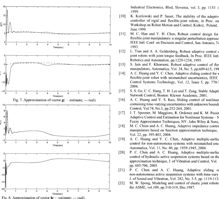
Fig. 3 is the joint space tracking performance. It shows that the transient response vanishes very quickly. Fig. 4 is the actuator inputs in N-m. Fig. 5 to 8 are the performance of function approximation for D, C, g and h respectively. Since the reference input does not satisfy the persistent excitation condition, some estimates do not converge to their actual values but remain bounded as desired. It is worth to note that in designing the controller we do not need much knowledge for the system. All we have to do is to pick some controller parameters and some initial weighting ^matrices.

IV. CONCLUSIONS

In this paper, we have proposed a FAT-based adaptive controller for a flexible joint robot containing time-varying uncertainties. The new design is free from regressor calculation and knowledge of bounds of uncertainties.

Feedback of the joint acceleration is also avoided. The function approximation technique is used to deal with time-varying uncertainties. Using the Lyapunov like analysis, rigorous proof of the closed loop stability has been investigated with consideration of the approximation error.

Computer simulation results justify its feasibility of giving satisfactory tracking performance on a 2-D flexible-joint robot although we do not know much knowledge about the system model.

III. SIMULATION STUDY

Consider a planar robot (Fig. 1) with two rigid links and

T T s T

v < e.

^e

⁺ t5, Ils11 ⁺ 45, ^{e .}

40 _

a 20

-20 0 1 2 3 4 5 6 7 8 9 1

Time(sec)

100.

50

20

-50

-100

Fig. 1. 2-DOF planar robot

0.55 0.6 0.65 0.7 0.75 0.8 0.85 0.9 0.95

1

1.05

x

Fig. 2. Tracking performance of end-point in the Cartesian

space

(- actual;

--- desired). Initial position of end-point is at the point (0.6m, 0.6m). After

some transient, the tracking error is very small, although we do not know precise dynamics of the robot.

0.6-

0.4- a-'0

° 0.2-

5 6 7

Time(sec)

1 2

3 4 5 6

Time(sec)

0

0.8-

0.6

c

0.4

0.2

0

-

0

0.3, 0.25 0.2

C

0.15

C) 0.1 /

0.05

2 3 4 5 6 7 8 9 10

Time(sec)

Fig. 4. Actuator input.

0.25 0.2

0.. 0.15 01

2 4 6 8 1

Time(sec)

/

0

-0.05 1.

-0.1

0.12 0.115 0.11

2" 0. 105 0.1 0.095

2 4 6 8 1

Time(sec)

-0.05' 0.09

0 2 4 6 8 10 0 2 4 6 8 10

Time(sec) Time(sec)

Fig. 5. Approximation of D matrix(- estimate; --- real).

Although the estimated values do not converge to the true values, they are bounded and small.

0.4 0.3 0.2 01 03 0.2

__

O 01 __

-0.1

0 2 4 6 8 10

Time(sec)

0.151 0.1

Z) 0.05

-0.05

0.3

0.2

0.1

\

0-

-0.1 0 2 4 6 8 10

Time(sec)

0.2 0.15 0.1 02 '9 0.05

C)

0 -0.05

-0.1' -0.1I

0 2 4 6 8 10 0 2 4 6 8 10

Time(sec) Time(sec)

Fig. 6. Approximation of C matrix(- estimate; --- real).

7 8 9 10

Fig. 3. The joint space tracking performance(- actual;

^---

desired).

The real trajectory converge to the desired are very quickly.

1.2

1.1

>

0.9

0.8

0.7

0.6

*v 1.5

C-d

1

0-a

co

0.5

'6

60

-150

1.3

~

ns

2

n

I

0

1

C,j

11

15

-

10

5

0 1 2 3 4 5 6 7 8 9 1C

Time(sec)

5r I,

C

-10

-1 5 0 1 2 3 4 5 6 7 8 9 10

Time(sec)

Fig. 7. Approximation of vector g(- estimate; --- real).

10 8 6 4 2 0

-2 0 1 2 3 4 5 6 7 8 9 10

Time(sec)

51

8 9 10

0 -5

-10

-15

-zv

0 1 2 3 4 5 6 7

Time(sec)

Fig. 8. Approximation of vector h(- estimate; --- real).

Industrial Electronics, Bled, Slovenia, vol. 3, pp. 1153 -1158, July 1999.

[10] K. Kozlowski and P. Sauer, The stability of the adaptive tracking controller of rigid and flexible-joint robots, in Proc. on the First Workshop on Robot Motion and Control, Kiekrz, Poland, pp. 85-93, June 1999.

[11] M. C. Han and Y. H. Chen, Robust control design for uncertain flexible-joint manipulators: a singular perturbation approach, in Proc.

IEEE Intl. Conf. on Decision and Control, San Antonio, Texas, Dec.

1993.

[12] L. Tian and A. A. Goldenberg, Robust adaptive control of flexible joint robots with joint torque feedback, In Proc. IEEE Intl. Conf. on Robotics and Automation, pp.1229-1234, 1995.

[13] S. Jain and F. Khorrami, Robust adaptive control of flexible-joint manipulators, Automatica, Vol. 34, No. 5, pp.609-615, 1998.

[14] A. C. Huang and Y. C. Chen, Adaptive sliding control for single-link flexible-joint robot with mismatched uncertainties, IEEE Trans. on Control Systems Technology, Vol. 12, Issue 5, pp. 770-775, Sept.

2004.

[15] S. S. Ge, C. C. Hang, T. H. Lee and T. Zang, Stable Adaptive Neural

° Network Control, Boston: Kluwer Academic, 2001.

[16] A. C. Huang and Y. S. Kuo, Sliding control of nonlinear systems containing time-varying uncertainties with unknown bounds, Int. J. of Control, Vol.74, No.3, pp.252-264, 2001.

[17] J. T. Spooner, M. Maggiore, R. Ordonez and K. M. Passino, Stable Adaptive Control and Estimation for Nonlinear Systems

-

Neural and Fuzzy Approximator Techniques, NY: John Wiley & Sons, 2002.

[18] M. C. Chien and A. C. Huang, Adaptive impedance control of robot manipulators based on function approximation technique, Robotica, Vol. 22, pp. 395403, 2004.

[19] A. C. Huang and Y. C. Chen, Adaptive multiple-surface sliding

° control for non-autonomous systems with mismatched uncertainties, Automatica, Vol. 1, No.40, pp. 1939-1945, 2004.

[20] P. C. Chen and A. C. Huang, Adaptive multiple-surface sliding control of hydraulic active suspension systems based on the function approximation technique, J. of Vibration and Control, Vol. 11, No. 5, pp. 685-706, 2005.

[21] P. C. Chen and A. C. Huang, Adaptive sliding control of non-autonomous active suspension systems with time-vary loadings, J. of Sound and Vibration, Vol. 282, No. 3-5, pp. 1119-1135,2005.

[22] M. W. Spong, Modeling and control of elastic joint robots, Tran. of the ASME, vol.109, pp.310-319, Dec.1987.

REFERENCES

[I] L. M. Sweet and M. C. Good, Redefinition of the robot motion control problem: effects of plant dynamics, drive system constraints, and user requirements, in Proc. IEEI Int. Conf. of Decision and Control, Las Vegas, pp. 724-730, 1984.

[2] M. W. Spong, Adaptive control of flexible-joint manipulators, Systems and Control Letters, vol. 13, pp.15-21, 1989.

[3] M. W. Spong, Adaptive control of flexible-joint manipulators:

Comments on two papers, Automatica, vol.31, no. 4, pp.585-590, 1995.

[4] K. P. Chen and L. C. Fu, Nonlinear adaptive motion control for a

manipulator with flexible-joints, In Proc. IEEE Intl. Conf. on Robotics and Automation, Phoenix, Az., pp. 1201-1206, May 1989.

[5] K. Khorasani, Adaptive control of flexible-joint robots, IEEE Trans.

on robotics and Automation, Vol. 8, No. 2, pp. 250-267, April, 1992.

[6] S. Y. Lim, D. M. Dawson, J. Hu, and M. S. de Queiroz, An adaptive link position tracking controller for rigid-link flexible-joint robots without velocity measurements, IEEE Trans. on System, man, and Cybernetics-Part B: Cybernetics, vol. 27, No. 3, June 1997.

[7] W. E. Dixon, E. Zergeroglu, D. M. Dawson and M. W. Hannan, Global adaptive partial state feedback tracking control of rigid-link flexible-joint robots, in Proc. IEEE/ASME Intl. Conf. on Advanced Intelligent Mechatronics, Atlanta, GA, pp. 281-286, Sept. 1999.

[8] W. Yim, Adaptive control of a flexible-joint manipulator, In Proc.

IEEE Int. Conf. on Robotics and Automation, pp.3441-3446, 2001.

[9] K. Kozlowski and P. Sauer, On adaptive control of flexible-joint manipulators: theory and experiments, in Proc. IEEE Intl. Sym. on 201

-Po I