Focusing or Balancing? The Resource Allocation Problem for
Demand Forecasting and Performance Measurement
∗Ling-Chieh Kung and Ying-Ju Chen†
Abstract
We consider a retailer investing in two monitoring functions for unobservable demand and salesperson’s effort. We show that improving effort monitoring is more effective. Moreover, demand monitoring may be less preferable when it becomes relatively cheaper and balancing these two may be worse when they become more complementary.
Keywords: information asymmetry, demand forecasting, performance measure-ment, resource allocation.
1
Introduction
Over decades, motivating salespeople to exert costly effort has been known to be challenging due to the unobservability of the sales effort. As the sales effort is unobservable, a retailer can only compensate her salespeople contingent on the sales outcome. Thus, she inevitably rewards or punishes a salesperson’s luck rather than his effort, thereby leading to inefficient effort exertion that hurts the retailer. The inefficiency is further aggravated when the salesperson can privately observe the market condition due to either his past experience or local expertise. Since the retailer cannot distinguish between a good market condition and the salesperson’s hard working from the realized sales outcome, outcome-based compensation may be even more biased.
The retailer in the above scenario faces two well-documented information problems in eco-nomics: the adverse selection problem regarding the market condition and the moral hazard prob-lem regarding the sales effort. While the mixture of adverse selection and moral hazard results in an inefficient level of sales effort, two monitoring functions of information systems, demand
∗We thank Sridhar Seshadri (the area editor) and the review team for their detailed comments and many valuable
suggestions that have significantly improved the quality of the paper. All remaining errors are our own.
†Department of Industrial Engineering & Operations Research, University of California, Berkeley, CA 94720; tel:
510-642-2497; fax: 510-642-1403; e-mail:{lckung, chen}@ieor.berkeley.edu
forecasting and performance measurement, are helpful in alleviating adverse selection and moral hazard, respectively. The adoption of the two functions confronts the retailer with an intriguing
resource allocation problem. As software vendors typically provide modularization/customization
and allow a retailer to choose a mix of the two functions, three possible strategies are available for a retailer to allocate her fixed budget. She may choose the “focusing-on-demand ” strategy by allocating all the budget to demand forecasting, the “focusing-on-effort ” strategy by investing everything in performance measurement, or the “balancing” strategy by dividing the budget for the two functions. In other words, the retailer needs to decide whether to become an expert in one aspect but know little for the other or obtain intermediate accuracy in monitoring both.
To address this question, we construct a stylized supply chain with a retailer (principal) and a salesperson (agent). The salesperson’s effort level affects the final sales outcome. While the salesperson chooses his effort level in response to the compensation scheme offered by the retailer, the retailer designs the contract according to her estimate of the market condition and the sales effort. Before she designs the contract, the retailer invests in demand forecasting and performance measurement to obtain two estimators, one for the market condition and one for the sales effort. It is assumed that the two functions may be complementary, which means enhancing the accuracy of one of them makes the other one less expensive. The retailer’s goal is to optimally invest in the two functions so that she can maximize her expected profit.
The analysis of the resource allocation problem starts with the embedded contract design problem. By taking the salesperson’s response into consideration, we characterize the retailer’s optimal contract and explicitly formulate the resource allocation problem. It is then shown that improving the accuracy of effort monitoring can induce a higher effort level and generate more profits in expectation. In the extreme case, if effort monitoring is perfectly precise, there will be no efficiency loss regardless of the accuracy of demand monitoring. These results suggest that effort monitoring is more effective than demand monitoring. However, the resource allocation problem is analytically challenging to solve and arguably even intractable. Therefore, we resort to numerical studies to discuss factors that influence the retailer’s monitoring decision.
We find that the costs of improving accuracy affect the retailer’s decision in a nonintuitive way: As the cost of effort monitoring increases, focusing on demand becomes less attractive. Because the total investments of the two functions cannot exceed the fixed budget, any cost increment worsens the three strategies (focusing-on-effort, focusing-on-demand, and balancing) simultaneously. In particular, if the retailer focuses on the demand, the cost increment results in a precision loss in effort monitoring. As effort monitoring is more effective than demand monitoring, such a precision loss harms the retailer the most among the three strategies. Another interesting observation is that the balancing strategy is not always preferable with a high degree of complementarity. Instead,
becoming an expert in one side and utilizing the high complementarity to understand the other side may be more beneficial. In particular, when there is a high physical restriction or a high cost on effort monitoring, focusing on demand is the most efficient way to monitor the sales effort if the two functions are sufficiently complementary. Balancing thus becomes less preferable.
Our paper falls into the interface between marketing and operations. How performance mea-surement may facilitate salesforce management has been a central topic in the marketing literature [1, 6, 7]. On the other hand, researchers in operations management have shown that demand fore-casting can alleviate demand uncertainty and therefore benefit a firm or the whole supply chain [2, 3, 11]. In a recent contribution, Sohoni et al. [15] consider the scenario in which the dealer is paid on a per unit basis when the total sales exceeds a threshold value; a fixed bonus may also be offered. In a dynamic setting, Sohoni et al. [14] investigate the hockey stick phenomenon commonly observed in practice. Nevertheless, no study has investigated the resource allocation problem re-garding demand forecasting and performance measurement simultaneously. Because the resource allocation problem has an embedded contract design problem, our study also contributes to the vast literature on salesforce management and staffing policies (cf. the comprehensive review [12]). The issue of what to monitor, especially the choice between input-based (effort level) and output-based (sales outcome) compensations, has been studied before in the economics literature. The seminal paper by Holmstrom and Milgrom [5] considers a multi-tasking problem and shows that it is typically suboptimal to make the compensation entirely based on the inputs. Zhao [16] shows that if the principal cannot monitor all the inputs (efforts for all the tasks) by the agent, then output-based compensation should be applied. There are also other studies that address the relationship between hidden information and hidden action by comparing input-based and output-based compensations (e.g. [10, 13]). Nevertheless, none of the aforementioned papers considers the possibility of allowing the principal to mitigate both the hidden information and the hidden action, which is the primary objective of our paper. The effort exertion in a decentralized channel has been widely discussed in the operations research literature (see [4, 8], among others). To the best of our knowledge, the resource allocation problem has no counterpart in this stream.
The rest of this paper is organized as follows. In Section 2, we describe the model setting and assumptions. The retailer’s contract design and resource allocation problems are formulated and analyzed in Section 3. We perform numerical studies in Section 4 to generate more insights.
2
Model
We consider a supply chain in which a retailer (she) relies on a salesperson (he) to sell the products. The supply chain is operated in a make-to-order (MTO) manner, in which the retailer can determine
the procurement quantity after the demand realization. Without loss of generality, we normalize the unit procurement cost to 0 and the unit retail price to 1. While the retailer is risk-neutral and maximizes her expected profit, the salesperson is risk-averse and maximizes his expected utility. The salesperson’s risk preference is represented by a negative exponential utility function U (z) =−e−ρz, where ρ > 0 is the coefficient of absolute risk aversion and z is his net income. The salesperson’s (risk-free) reservation net income is normalized to zero without loss of generality.
While the salesperson is able to observe the realization of the market condition, he may further enhance the sales outcome by exerting effort. Specifically, the sales outcome x is determined by a normally distributed market condition θ∼ N(µθ, σθ2), the salesperson’s sales effort a, and a random noise ϵ in the following additive form
x = θ + a + ϵ, (1)
where ϵ∼ N(0, σϵ2). We assume that µθ > 0, σ2θ > 0, σ2ϵ > 0, and the probability of x being negative is sufficiently small. To exert effort a, the salesperson incurs a cost 12a2, where the quadratic form is made for simplicity. The functional form (1), the cost of effort 12a2, the parameters µθ, σθ2, and
σ2ϵ, and the realized sales outcome x are all common knowledge. However, the market condition θ and the sales effort a are not observable by the retailer.
The retailer may invest in demand forecasting and obtain an estimator s = θ +τ for θ. She may then use the estimate s to update her belief on the market condition. The retailer may also invest in performance measurement and estimate the sales effort through the estimator q = a + ξ. We assume that τ ∼ N(0, στ2) and ξ∼ N(0, σξ2). The two variance terms στ2> 0 and σξ2> 0 are referred
to the retailer’s monitoring accuracy of demand monitoring and effort monitoring, respectively. In what follows, we refer to s as the demand signal. It is also assumed that τ is independent of θ, ξ is independent of a, and τ and ξ are independent. Because the salesperson is an employee of the retailer, in practice he knows the estimation made by his company. Therefore, we assume that the realized value of s and q as well as all the distributions are common knowledge.
For the monitoring accuracy, we impose the feasibility constraints στ2 ≥ Kτ and σξ2 ≥ Kξ with Kτ ≥ 0 and Kξ≥ 0 being exogenous parameters. These constraints incorporate the physical restrictions that the retailer may encounter in improving accuracy in either aspect. In addition, the retailer faces a resource constraint in allocating her budget to these two functions. With C being the total budget and g(σ2τ, σξ2) being the cost for achieving στ2 and σξ2, the retailer’s resource constraint is g(στ2, σξ2) ≤ C. It is assumed that g increases as στ2 or σ2ξ decreases because more accurate estimators should be more expensive. g is also assumed to be jointly convex in στ2 and
σ2ξ so that improving accuracy is more costly when the accuracy is already high. As we will see in Section 4, the convexity also allows us to incorporate the complementarity between the two aspects. In the retailer-salesperson relationship, we restrict our attention to the class of linear contracts
that are prevalent in practice. Specifically, we use (α, β, w) to denote the contract signed by the retailer and the salesperson, where α is a fixed payment, β is a commission rate regarding the sales outcome x, and w is an input bonus rate based on the estimate q. With this contract, the salesperson receives an aggregate payment α + βx + wq if sales outcome x and effort estimate q are realized. Since the retailer is unable to observe the market condition θ, her best strategy is to offer a menu of contracts for the salesperson to self-select and reveal θ truthfully. The menu of contracts offered by the retailer is thus denoted as{α(θ), β(θ), w(θ)}. Note that the retailer will design the contract based on her posterior belief on the market condition.
The sequence of events is summarized in Figure 1: 1) The retailer decides her monitoring accuracy σ2
τ and σξ2; 2) θ is realized and privately observed by the salesperson. The two players then observe the demand signal s. 3) Based on the signal s and the accuracy σ2
τ, the retailer updates her posterior belief on θ to θ|s and announces a compensation scheme {α(·), β(·), w(·)} to her salesperson; 4) The salesperson chooses a contract (α, β, w) based on θ and s he observes or rejects this offer; 5) If the salesperson rejects the contract, the game ends and each player receives a null payoff. Otherwise, the selling season starts, the salesperson exerts sales effort a, the retailer gets the effort estimate q, the sales quantity x is realized, and the salesperson is rewarded accordingly.
-Reseller chooses σ2 τ and σ2ξ θrealizes and sis observed
Reseller updates her belief on θ to θ|s and
offers {α(·), β(·), w(·)}
Salesperson chooses a contract or rejects the offer
Salesperson chooses a, reseller obtains q, x realizes, and salesperson is rewarded
Figure 1: Sequence of events
3
Analytical results
3.1 The contract design problem
Consider the salesperson’s problem for a given menu of contracts first. Suppose that the true market condition is θ but the salesperson chooses the contract (α(˜θ), β(˜θ), w(˜θ)) by reporting a false market
condition ˜θ, then by exerting effort a, his net income will be z(a) = α(˜θ)+β(˜θ)(θ+a+ϵ)+w(˜θ)q−12a2. Given z(a), the salesperson’s expected utility isE[−e−ρz(a)]=−e−ρCE(θ,˜θ|a), where
CE(θ, ˜θ|a) = α(˜θ) + β(˜θ)(θ + a) + w(˜θ)a −1
2a 2−1 2ρ[β(˜θ)] 2σ2 ϵ − 1 2ρ[w(˜θ)] 2σ2 ξ
is called the salesperson’s certainty equivalent. Let CE(θ, ˜θ) ≡ maxa≥0CE(θ, ˜θ|a). Because the exponential function is monotonic, the salesperson can maximize his expected utility by choosing
a∗(˜θ) = β(˜θ) + w(˜θ) to maximize the certainty equivalent. With this optimal effort level, the
salesperson receives his maximum certainty equivalent
CE(θ, ˜θ) = α(˜θ) + β(˜θ)θ + [ β(˜θ) + w(˜θ) ]2 −1 2ρ [ β(˜θ) ]2 σϵ2− 1 2ρ [ w(˜θ) ]2 σξ2. (2) Let CE(θ)≡ CE(θ, θ).
With the salesperson’s response in mind, the retailer considers her contract design problem as follows. First, from the representation s = θ + τ , she applies Bayesian inference to derive the posterior belief of θ given s. With σ2 ≡ σ2τ/(στ2 + σ2θ), the conjugate property of normal distributions leads to the posterior distribution θ|s ∼ N
(
σ2µθ+ (1− σ2)s, σθ2σ2 )
. Denote F (θ|s),
f (θ|s), and H(θ|s) ≡ 1−F (θ|s)f (θ|s) as the distribution, density, and inverse failure functions of the posterior distribution θ|s. In equilibrium, the salesperson observing θ will choose the contract (α(θ), β(θ), w(θ)) that is intended for him. The retailer then pays β(θ)(θ + a(θ)) as the expected sales commission, w(θ)a(θ) as the expected input compensation, and α(θ) as the fixed payment. Therefore, conditioning on the observed demand signal s, she maximizes her expected profit by solving max {α(θ) urs, β(θ)≥0, w(θ)≥0} Eθ|s [ (1− β(θ))[θ + β(θ) + w(θ)] − w(θ)[β(θ) + w(θ)] − α(θ)|s ] (3) s.t. CE(θ)≥ CE(θ, ˜θ) ∀θ, ˜θ ∈ (−∞, ∞), (4) CE(θ)≥ 0 ∀θ ∈ (−∞, ∞), (5)
where the incentive compatibility (IC) constraint (4) guarantees truth-telling and the individual rationality (IR) constraint (5) guarantees the salesperson’s participation.
To solve this problem, first note that ∂θ∂CE(θ) = β(θ)≥ 0. Therefore, CE(θ) is nondecreasing
in θ. To satisfy the IR constraint (5), at optimality we have CE(−∞) = 0 and CE(θ) =∫−∞θ β(y)dy.
By ignoring the IC constraint (4), we may apply CE(θ) =∫−∞θ β(y)dy and the expression of CE(θ)
in (2) to reduce the problem to max {β(θ)≥0, w(θ)≥0} Eθ|s [ θ+β(θ)+w(θ)−(β(θ) + w(θ)) 2 2 − 1 2ρ ( β(θ)2σϵ2+w(θ)2σ2ξ ) −H(θ|s)β s ] (6) with integration by parts applied. Because this objective function is concave on β(θ) and w(θ), the first-order condition is sufficient and the optimal solutions β∗(θ) and w∗(θ) satisfy 1− (β∗(θ) +
w∗(θ))− ρβ∗(θ)σϵ2− H(θ|s) = 0 and 1 − (β∗(θ) + w∗(θ))− ρw∗(θ)σξ2= 0. With β∗(θ)≥ 0 in mind, solving the two equations leads to
w∗(θ) = 1− β ∗(θ) 1 + ρσ2ξ and β ∗(θ) = [ ρσ2ξ− (1 + ρσ2ξ)H(θ|s) ρσξ2+ (1 + ρσξ2)ρσ2 ϵ ]+ . (7)
Note that β∗(θ) ≤ 1, which implies w∗(θ) ≥ 0. The optimal fixed payment α∗(θ), which can be derived by plugging β∗(θ) and w∗(θ) into (2) and applying CE(θ) =∫−∞θ β(y)dy, is
α∗(θ) =−β(θ)θ −[β(θ) + w(θ)] 2 2 + 1 2ρ [ β(θ)2σ2ϵ + w(θ)2σ2ξ ] + ∫ θ −∞β(y)dy. (8) It then follows that the induced effort level is a∗(θ) = β∗(θ) + w∗(θ). Verifying the IC constraint is trivial and omitted.
The menu of contracts aims to differentiate salespeople observing different market conditions. A high-type salesperson (observing a good market condition) prefers a high commission rate because he is optimistic about the sales outcome. Therefore, the retailer finds it optimal to cut down the commission rate β∗(θ) intended for low-type salespeople (observing a bad market condition). This is captured by the inverse failure function H(θ|s), which is decreasing in θ for the normal distribution. The input compensation w∗(θ), on the contrary, is decreasing in θ. The reason for a high-type salesperson to prefer a high commission rate rather than a high input bonus rate is clear: High commission may be earned with luck but high input bonus definitely requires the costly effort. Since a high-type salesperson believes the market condition is good, he is willing to accept a low input bonus rate in exchange of a high commission rate. Reducing the input bonus rate for high-type salespeople thus helps the retailer make a better differentiation. Note that the induced effort level a∗(θ) is jointly determined by β∗(θ) and w∗(θ) in an additive form. Though the decreasing
w∗(θ) lowers the effort level when θ becomes larger, the reduction is dominated by the incentive brought by β∗(θ). Therefore, high-type salespeople are willing to work harder.
Intuitively, the retailer should be able to induce a higher expected effort level by improving her monitoring accuracy. The following lemma confirms the intuition for effort monitoring.
Lemma 1. When σξ2 decreases, β∗(θ) decreases, w∗(θ) increases, and a∗(θ) increases for all θ. In
addition, E[a∗(θ)] strictly increases as σ2ξ decreases.
Proof. Consider β∗(θ) first. Because H is strictly decreasing from infinity to 0, we define θ0 as the
unique value satisfying H(θ0|s) =
ρσ2
ξ
1+ρσ2
ξ
. It then follows that β∗(θ) = 0 for all θ≤ θ0and β∗(θ) > 0
for all θ > θ0. Note that when σξ2 increases,
ρσ2ξ
1+ρσ2
ξ
increases, so θ0 decreases. This implies that
β∗(θ) is weakly increasing in σ2
ξ for all θ≤ θ0: It either remains 0 or becomes positive. For θ > θ0,
we have ∂β∂σ∗(θ)2
ξ
= ρσϵ2+H(θ|s)
ρ(σ2
ξ+σ2ϵ+ρσ2ξσ2ϵ)2 > 0. Therefore, we conclude that β
∗(θ) decreases as σ2
ξ decreases for all θ. Because w∗(θ) = 11+ρσ−β∗(θ)2
ξ
, it is now clear that w∗(θ) increases as σξ2 decreases for all θ. Finally, consider a∗(θ). We have a∗(θ) = β∗(θ) + w∗(θ) = 1+β∗(θ)ρσ
2 ξ 1+ρσ2 ξ . For θ≤ θ0, β∗(θ) = 0 and it is clear that a∗(θ) = 1+ρσ1 2 ξ
increases as σξ2 decreases. For θ > θ0, we have ∂a
∗(θ) ∂σ2 ξ = σ 2 ξ[−ρσϵ2−H(θ|s)] (σ2 ξ+σϵ2+ρσξ2σϵ2)2 < 0.
Therefore, a∗(θ) decreases as σ2ξ decreases for all θ. The result forE[a∗(θ)] follows.
Compared with the sales commission, which is affected by the market condition, the risk-averse salesperson typically prefers to be rewarded through the more controllable input bonus. However, this is only the case when the retailer’s effort monitoring is precise. Therefore, once the retailer improve her effort monitoring accuracy, the two parties will agree on a lower commission rate and a higher input bonus rate. More interestingly, though the effort level is determined by the two opposite forces, the positive effect brought by increasing the input bonus rate always dominates the negative effect of decreasing the commission rate. The salesperson will thus be willing to work harder. As this is true for all possible values of θ, the expected induced effort level is increased. This lemma thus provides a simple guideline for the retailer: Investing more in effort monitoring directly helps the retailer better motivate the salesperson.
Having obtained the retailer’s optimal menu of contracts, we now proceed to her resource allocation problem.
3.2 The resource allocation problem
By offering the optimal contracts, the retailer’s expected profit given her choice of the monitoring accuracy is R(στ2, σ2ξ)≡ Es { Eθ|s [ (1− β∗(θ))(θ + a∗(θ))− w∗(θ)a∗(θ)− α∗(θ) s ]} ,
where α∗(θ), β∗(θ), and w∗(θ) are defined in (7) and (8) and a∗(θ) = β∗(θ) + w∗(θ). Inside the expectation over s is the maximized objective function (3) of the contract design problem. Because the demand signal s has not been observed when the retailer makes the choice of monitoring accuracy, she takes expectation over s, whose realization depends on the accuracy σ2τ. The retailer’s resource allocation problem is thus formulated as
max σ2 τ,σ2ξ { R(στ2, σξ2) στ2≥ Kτ, σξ2≥ Kξ, g(σ2τ, σξ2)≤ C } . (9)
The complicated structure of the optimal menu of contracts prohibits us from analytically solving (9) completely. Furthermore, finding the optimal accuracy mix may be numerically challenging as well because in essence we need to conduct a two-dimensional numerical search. Fortunately, the structural property stated in the following proposition allows us to obtain a clear insight and largely reduce the search space.
Proposition 1. In the retailer’s resource allocation problem (9), the expected profit R(στ2, σξ2)
Proof. For ease of notation, denote f (θ) by f for f ∈ {α, β, w} in this proof when there is no ambiguity. Recall that in solving the contract design problem (3) – (5), the first step is to replace
α by β and w and obtain (6). Therefore, we may express the expected profit as R(στ2, σ2ξ) = Es { max β≥0, w≥0 Eθ|s [ θ + β + w−(β + w) 2 2 − 1 2ρ(β 2σ2 ϵ + w2σξ2)− H(θ|s)β s ]} .
Note that those terms inside the expectation over s appear in (6) exactly in the same way. For every realization of s, the retailer looks for β and w to maximize her expected profit. Let h(β, w, σ2ξ) ≡
θ + β + w− (β+w)2 2 − 12ρ(β2σ2ϵ + w2σ2ξ) − H(θ|s)β be the integrand, which decreases in σξ2 if
β and w are fixed. It follows that the expectation to be maximized, Eθ|s [
h(β, w, σξ2)|s ]
, also decreases in σξ2. Let ¯σ2ξ < ˆσξ2 be two values of σξ2, we know maxβ≥0, w≥0
{ Eθ|s [ h(β, w, ¯σ2ξ)|s ] } > maxβ≥0, w≥0 { Eθ|s [ h(β, w, ˆσξ2)|s ] }
since these two optimization problem have the same feasible region and the objective function of the former is larger than that of the latter for every feasible solution. In other words, for any given s, the retailer can do better in expectation with a smaller
σ2ξ. Since this is true for every realization of s, it is true for the expectation of s. Therefore,
R(σ2τ, ¯σξ2) > R(στ2, ˆσ2ξ) and we conclude that R(στ2, σξ2) strictly decreases in σ2ξ.
As we have seen in Lemma 1, with a higher accuracy of effort monitoring, the retailer can better motivate the salesperson, ultimately benefiting the end consumers. Proposition 1 further shows that the retailer is strictly better off when she improves the accuracy. Therefore, a larger amount of investment in effort monitoring benefits both the end consumer and the retailer. This demonstrates the benefits, from the retailer’s perspective, of resolving the moral hazard problem. As long as it is still possible to improve the accuracy of effort monitoring (without worsening demand monitoring), the retailer should invest more to do so.
Proposition 1 offers another technical implication. Because R(σ2τ, σξ2) decreases in σξ2, any feasible accuracy mix satisfying g(σ2τ, σξ2) < C and σξ2 > Kξ can be improved by decreasing στ2. Therefore, at least one of the constraints g(στ2, σξ2)≤ C and σξ2≥ Kξ will be binding at optimality. This necessary condition for the optimal solution is summarized in the following corollary.
Corollary 1. In the retailer’s resource allocation problem (9), at least one of the constraints
g(σ2τ, σξ2)≤ C and σ2ξ ≥ Kξ is binding at the optimal solution.
This necessary condition partially resolves the complexity of the underlying resource alloca-tion problem as it allows us to discard a large class of candidate solualloca-tions that are never optimal. Unfortunately, even with this necessary condition, the general problem (9) cannot be solved ana-lytically. We thus investigate the general case numerically in Section 4. Nevertheless, to gain more managerial insights, we first analytically compare two special solutions, which correspond to the
two extreme ways of monitoring: perfect demand monitoring and perfect effort monitoring. More precisely, we have σ2τ = 0 but σξ2 → ∞ in the first solution and σ2ξ = 0 but στ2 → ∞ in the second solution. The next proposition summarizes the results under the two solutions. Note that the retailer adopting perfect demand monitoring does not include the input bonus w in the contract since the effort is no longer measurable.
Proposition 2. With perfect demand monitoring and the observed demand signal s, the retailer
offers αD = 12(βD)2(1− ρσϵ2)− βDs and βD = 1+ρσ1 2
ϵ, induces effort level a
D = 1 1+ρσ2
ϵ, and receives
expected profit RD = µθ+ 2(1+ρσ1 2
ϵ). With perfect effort monitoring, the retailer offers α
E = −1 2,
βE = 0, and wE = 1, induces effort level aE = 1, and receives expected profit RE = µθ+12. Proof. For perfect demand monitoring (στ2 = 0), the true market condition θ is not a private information of the salesperson and the adverse selection problem no longer exists. It is thus sufficient for the retailer to offer a single contract (α, β) to the salesperson. Given (α, β) and θ, the salesperson maximizes his certainty equivalent CED(θ|a) = α+β(θ+a)−12a2−12ρσϵ2β2by choosing the optimal effort level a = β. His maximum certainty equivalent is thus CED(θ) = α+βθ +12β2(1−ρσϵ2). With this, the retailer solves RD(θ) = maxα urs,β≥0
{
(1− β) (θ + β) − α α + βθ + 12β2(1− ρσϵ2)≥ 0 }
.
Since the constraint must be binding at optimality, the problem can be reduced to an unconstrained problem with β as the only variable. By the first order condition, the optimal commission rate
βD(θ) = 1+ρσ1 2
ϵ determines the induced effort level a
D(θ) = 1 1+ρσ2 ϵ. Consequently, R D(θ) = θ + 1 2(1+ρσ2 ϵ) and R D = E[RD(θ)] = µ θ + 2(1+ρσ1 2
ϵ). For perfect effort monitoring, the retailer can
still incorporate the three elements in the contract. It then follows that the optimal contract is simply the limit of the solution in (7). With σξ2 = 0 and στ2 approaches infinity, we have
β(θ)→ [ −H(θ) 1+ρσ2 ϵ ]+
= 0, w(θ)→ 1, and α(θ) → −12. Therefore, the induced effort level is a(θ) = 1
and the expected profit is RE = µ θ+12.
In the case of perfect demand monitoring, the only source of effort distortion follows from the pure moral hazard problem (as captured by the term 1+ρσ1 2
ϵ) faced by the retailer. This downward
distortion in commission rate limits the risk premiums necessary to compensate the salesperson for bearing risk. As the salesperson is more risk averse (ρ increases) and the market condition is more volatile (σϵ2 increases), more risk premiums are required and thus a larger downward distortion arises in the commission rate. On the other hand, perfect effort monitoring results in no effort distortion. Because the sales effort can be enforced by the contractual agreement, the retailer can simply choose the efficient effort level (aE = 1) and extract all the surplus by the fixed payment (αE =−12). Since the commission rate is zero, the salesperson bears no risk and the retailer can offer no risk premium to induce the salesperson’s participation. She may thus achieve a higher expected profit than with perfect demand monitoring.
A related result has been derived by Kung and Chen [9]. In that paper, the authors also consider the salesforce compensation problem under adverse selection (regarding the hidden market condition) and moral hazard (regarding the sales effort). However, their main focus is on a three-layer supply chain with a manufacturer, a retailer, and a salesperson. Without allowing the retailer to choose an accuracy mix as we do in this study, the authors consider only the two extreme cases we investigate in Proposition 2. Similar to the conclusion of Proposition 2, they also show that including a retailer with perfect effort monitoring is better than including one with perfect demand monitoring. Therefore, as it includes one additional player (the manufacturer) and examine the interaction among the three players, that paper can be viewed as an extension of the above proposition. This study, however, focuses on the two-layer setting and generalizes the polar cases to a continuous choice of accuracy mix. Each study is thus a complement of the other one.
In both studies, if the retailer can choose to eliminate either the adverse selection or moral hazard problem, eliminating moral hazard is more beneficial. This suggests that moral hazard creates a higher loss in the retailer’s expected profit and is relatively more critical in the retailer-salesperson relationship. Therefore, it is intuitive to conjecture that effort monitoring generally brings more benefits than demand monitoring. Nevertheless, because neither the above comparison nor the analysis in [9] examine the physical and resource constraints, the costs of these two functions are ignored. In particular, effort monitoring may be extremely expensive and not cost-effective to implement. To provide the full picture of this resource allocation problem, we resort to the numerical studies in the next section.
4
Numerical studies
The first step in conducting numerical studies is to choose a specific form of the resource constraint
g(σ2
τ, σξ2)≤ C, which restricts the variances σ2τ and σξ2to be not too small. To make our experiments more intuitive with respect to σ2
τ and σ2ξ, we adopt an equivalent no-less-than form ˜g(στ2, σ2ξ)≥ B, where ˜g is a concave function on σ2
τ and σ2ξ. In the following experiments, we adopt ˜
g(στ2, σξ2) = cτστ+ cξσξ+ cjointστσξ ≥ B (10) as the resource constraint, where cτ, cξ, and B are positive and cjoint is nonnegative. With the concavity in στ2 and σξ2, the first two terms introduce the increasing marginal cost in improving accuracy: Reducing σ2τ (σξ2) is more expensive when στ2 (σξ2) is already small. The values of cτ and
cξ adjust costs so that improving demand (effort) monitoring becomes more expensive if cτ (cξ) becomes smaller. The complementarity between σ2τ and σξ2 is incorporated by the multiplicative term cjointσξστ, where larger cjoint implies a higher degree of complementarity. In particular, the costs of the two functions are independent when cjoint= 0.
0.5 1 1.5 2 2.5 3 0.5 1 1.5 2 2.5 3 10.4 10.6 10.8 11 σξ2 στ2 Expected Profit
Figure 2: Expected profits
0.25 0.5 0.750 1 1.25 1.5 1.75 2 2.25 2.5 100 200 300 400 500 Kξ Number of Solutions FOE Balancing FOD Balancing FOE FOD Figure 3: Effect of Kξ
We start our numerical study by performing a preliminary experiment to address the relative effectiveness of demand monitoring and effort monitoring. For ρ, σ2θ, and σϵ2, we test each of them for values 0.5, 1, and 2 and generate 33 = 27 scenarios. We set µθ = 10 in all experiments. Ignoring the constraints in the resource allocation problem (9), Figure 2 illustrates the expected profit as functions of σ2τ and σ2ξ. To obtain a value for a pair of στ2 and σξ2 in these figures, we average the 27 values from all the scenarios. This figure shows that 1) improving effort monitoring (decreasing σξ2) is more profitable than improving demand monitoring (decreasing στ2), and 2) improving demand monitoring is not effective when effort monitoring is precise (σξ2 is close to 0). Therefore, effort monitoring generally brings more benefits in the absence of those constraints.
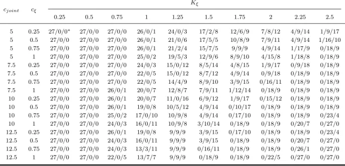
Now we provide a finer examination by adding the constraints back. Because effort monitoring is more beneficial in general, we fix B = 3 and cξ = 1 but adjust Kξ, cτ, and cjoint to introduce higher physical restrictions on effort monitoring, cheaper demand monitoring, and higher degrees of complementarity. For each of the 160 combinations of different values of Kξ, cτ, and cjoint(listed in Table 1), we test the 27 scenarios and count the frequencies of three types of optimal solutions: the focusing-on-demand solution (σ2
τ = Kτ, σ2ξ > Kξ; abbreviated as “FOD” below), the focusing-on-effort solution (σ2
τ > Kτ, σξ2 = Kξ; “FOE”), and the balancing solution (στ2 > Kτ, σξ2 > Kξ). See Table 1 for the complete result. Because none of these experiments results in a non-binding solution, we conclude that the resource constraint is binding at optimality for most of the time.
With these numerical results, we next analyze the effects of changing Kξ, cξ, and cjoint one by one. Figure 3 depicts how the retailer’s preference differs with different values of Kξ. From this figure, we find that FOE becomes less attractive when Kξ becomes larger, which is intuitive since the FOE solution is forced to be worse. When effort monitoring is still good enough (when Kξ is not too large), the retailer should partially switch to demand monitoring by adopting the balancing
cjoint cξ Kξ 0.25 0.5 0.75 1 1.25 1.5 1.75 2 2.25 2.5 5 0.25 27/0/0∗ 27/0/0 27/0/0 26/0/1 24/0/3 17/2/8 12/6/9 7/8/12 4/9/14 1/9/17 5 0.5 27/0/0 27/0/0 27/0/0 26/0/1 21/0/6 17/5/5 10/8/9 7/9/11 4/9/14 1/16/10 5 0.75 27/0/0 27/0/0 27/0/0 26/0/1 21/2/4 15/7/5 9/9/9 4/9/14 1/17/9 0/18/9 5 1 27/0/0 27/0/0 27/0/0 25/0/2 19/5/3 12/9/6 8/9/10 4/15/8 1/18/8 0/18/9 7.5 0.25 27/0/0 27/0/0 27/0/0 24/0/3 15/0/12 8/5/14 4/8/15 1/9/17 0/9/18 0/18/9 7.5 0.5 27/0/0 27/0/0 27/0/0 22/0/5 15/0/12 8/7/12 4/9/14 0/9/18 0/18/9 0/18/9 7.5 0.75 27/0/0 27/0/0 27/0/0 22/0/5 14/4/9 8/9/10 3/9/15 0/16/11 0/18/9 0/18/9 7.5 1 27/0/0 27/0/0 26/0/1 20/0/7 12/8/7 7/9/11 1/12/14 0/18/9 0/18/9 0/18/9 10 0.25 27/0/0 27/0/0 26/0/1 20/0/7 11/0/16 6/9/12 1/9/17 0/15/12 0/18/9 0/18/9 10 0.5 27/0/0 27/0/0 26/0/1 19/0/8 10/5/12 4/9/14 0/10/17 0/18/9 0/18/9 0/18/9 10 0.75 27/0/0 27/0/0 25/0/2 17/0/10 10/9/8 4/9/14 0/17/10 0/18/9 0/18/9 0/23/4 10 1 27/0/0 27/0/0 24/0/3 16/0/11 10/9/8 3/10/14 0/18/9 0/18/9 0/20/7 0/27/0 12.5 0.25 27/0/0 27/0/0 26/0/1 19/0/8 9/9/9 3/9/15 0/17/10 0/18/9 0/18/9 0/23/4 12.5 0.5 27/0/0 27/0/0 24/0/3 16/0/11 9/9/9 3/9/15 0/18/9 0/18/9 0/20/7 0/27/0 12.5 0.75 27/0/0 27/0/0 24/0/3 13/3/11 9/9/9 0/16/11 0/18/9 0/18/9 0/26/1 0/27/0 12.5 1 27/0/0 27/0/0 22/0/5 13/7/7 9/9/9 0/18/9 0/18/9 0/22/5 0/27/0 0/27/0
(∗x/y/z: the number of FOE/FOD/balancing solutions)
Table 1: Number of FOE, FOD, and balancing solutions
strategy. When effort monitoring is totally ineffective (Kξ is too large), the retailer will prefer to fully switch to demand monitoring. Balancing is thus attractive only when Kξ is moderate. The observation is summarized below.
Observation 1. Focusing on effort is preferred when Kξ is small, focusing on demand is preferred
when Kξ is large, and balancing is attractive when Kξ is moderate.
Now consider cξ, which represents the relative cost of effort monitoring. Intuitively, a higher cost in effort monitoring should drive the retailer to prefer the relatively cheaper demand monitor-ing. Nevertheless, Figure 4 shows the completely opposite trend.
Observation 2. When cξ decreases and effort monitoring is relatively more expensive, focusing on
effort and balancing become more preferable while focusing on demand becomes less attractive.
To understand this counterintuitive result, note that when one function becomes more expen-sive, both focusing solutions receive negative effects. To remain equally accurate in one side, the retailer will be forced to give up some precision in the other side due to the higher cost. Given that a precision loss in effort monitoring generally harms the retailer more (cf. Figure 2), it is reasonable for the retailer to prefer FOE more as effort monitoring becomes more expensive (cξ decreases). Note that balancing also becomes more profitable when cξ decreases. It is clear that this also results from the force driving the retailer to deviate from FOD.
0.25 0.5 0.75 1 150 200 250 300 350 400 450 500 550 600 650 cξ Number of Solutions FOE Balancing FOD Balancing FOD FOE Figure 4: Effect of cξ 5 7.5 10 12.5 150 200 250 300 350 400 450 500 550 600 650 cjoint Number of Solutions FOE Balancing FOD FOE Balancing FOD
Figure 5: Effect of cjoint
Interestingly, this observation shows that the effort monitoring function possesses the property of “Giffen goods”, i.e., the higher the price, the larger the consumption. In a typical example of Giffen goods, one may substitute meat by bread when bread becomes more expensive. This is because while bread is required for one’s daily life, meat is valuable mainly when there is enough bread. The choice between the two functions is similar: While effort monitoring is more direct, demand monitoring only creates marginal benefits. Therefore, the retailer should invest in demand monitoring only when she has extra money, i.e., when effort monitoring is cheap. If the cost of effort monitoring goes up and the current accuracy mix becomes infeasible, the retailer should substitute demand monitoring by the more critical effort monitoring. This explains the observation.
The last study is for the complementarity between the costs of demand monitoring and effort monitoring. Figure 5 gives rise to the following observation.
Observation 3. When the two functions become more complementary (cjoint increases), focusing
on effort becomes less profitable, focusing on demand becomes more profitable, and balancing becomes more profitable when cjoint is small but less profitable when cjoint is large.
The first part of this observation demonstrates the decreasing attractiveness of FOE as the degree of complementarity increases. Recall that effort monitoring is more effective than demand monitoring when they are independent. With complementarity, being precise in one aspect allows the retailer to monitor the other aspect more easily. Therefore, a higher degree of complementar-ity allows a focusing-on-demand retailer to utilize the effectiveness of effort monitoring. On the contrary, suppose that the retailer focuses on effort. It is indeed the case that the retailer can also
monitor demand more easily through complementarity. However, both Proposition 2 and Figure 2 suggest that improving demand monitoring offers only limited benefits when the accuracy of effort monitoring is already high. In short, complementarity is beneficial if the retailer focuses on demand but of the least value if she focuses on effort instead. It is thus profitable for the retailer to switch from FOE to FOD when it is highly complementary. This also explains the second part.
The third part deserves more attention. Intuitively, when the two aspects of monitoring become more complementary, we expect the retailer to prefer balancing more. To uncover the reason behind this nonmonotonicity of preference over the balancing strategy, we need to simultaneously consider Kξ, the physical restriction on the accuracy of effort monitoring, and cjoint, the degree of complementarity. From Figure 3, we know that balancing is attractive only when Kξ is moderate. Moreover, the previous paragraph explains why FOD is preferred when cjointis large. It is thus not surprising that in Table 1, the number of balancing solutions increases in cjoint only when Kξ is moderate and cjoint is not too large. In particular, when Kξ is large, a large cjointonly encourages the retailer to focus on demand and utilize the high degree of complementarity. In fact, when Kξ is so large that direct effort monitoring is impossible, FOD is the best way to monitor the effort (indirectly through the complementarity). In general, whether a higher cjointresults in a preference over the balancing strategy depends on the relationship between cjoint and Kξ.
As we have illustrated through the numerical studies, the physical restrictions on accuracy, the costs of improving accuracy, and the degree of complementarity all play roles in determining the op-timal accuracy mix. With those counterintuitive observations, our results show that the investment decision must be made carefully. In practice, we observe retailers implementing different investment strategies: some focus on demand forecasting, some care more about performance measurement, and some balance between these two. Our results may partially explain such a discrepancy.
References
[1] E. Anderson and R. Oliver. Perspectives on behavior-based versus outcome-based salesforce control systems. The Journal of Marketing, 51(4):76–88, 1987.
[2] Y. Aviv. The effect of collabortive forecasting on supply chain performance. Management
Science, 47:1326–1343, 2001.
[3] G. Cachon and M. Fisher. Supply chain inventory management and the value of shared information. Management Science, 46:1032–1048, 2000.
[4] F. Chen. Salesforce incentives, market information, and production/inventory planning.
[5] B. Holmstrom and P. Milgrom. Multitask principal-agent analyses: Incentive contracts, asset ownership, and job design. Journal of Law, Economics and Organization, 7:24–52, 1991. [6] K. Joseph and A. Thevaranjan. Monitoring and incentives in sales organizations: An
agency-theoretic perspective. Marketing Science, 17(2):107–123, 1998.
[7] M. Krafft. An empirical investigation of the antecedents of sales force control systems.
Mar-keting Science, 63(3):120–134, 1999.
[8] H. Krishnan, R. Kapuscinski, and D. Butz. Coordinating contracts for decentralized supply chains with retailer promotional effort. Management Science, 50(1):48–63, 2004.
[9] L. Kung and Y. Chen. Monitoring the market or the salesperson? the value of information in a multi-layer supply chain. Forthcoming in Naval Research Logistics, 2011.
[10] E. Lazear. The power of incentives. American Economic Review, 90(2):410–14, 2000.
[11] H. Lee, C. So, and C. Tang. The value of information sharing in a two-level supply chain.
Management Science, 46:626–643, 2000.
[12] M. Mantrala, S. Albers, F. Caldieraro, O. Jensen, K. Joseph, M. Krafft, C. Narasimhan, S. Gopalakrishna, A. Zoltners, R. Lal, and L. Lodish. Sales force modeling: State of the field and research agenda. Marketing Letters, 21(3):255–272, 2010.
[13] C. Prendergast. The tenuous trade-off between risk and incentives. Journal of Political
Econ-omy, 110(5):1071–1102, 2002.
[14] M. Sohoni, A. Bassamboo, S. Chopra, U. Mohan, and N. Sendil. Threshold Incentives and the Sales Hockey Stick. Forthcoming in Naval Research Logistics, 2010.
[15] M. Sohoni, S. Chopra, U. Mohan, and N. Sendil. Threshold Incentives and Sales Variance. Forthcoming in Production and Operations Management, 2010.