Efficient Routing Path Selection Algorithm based on Pricing Mechanism in Ad Hoc Networks

全文

(1)Efficient Routing Path Selection Algorithm based on Pricing Mechanism in Ad Hoc Networks Tzu-Chieh Tsai, Chien-Chi Lin Computer Science Department, National Chengchi University [email protected], [email protected] ABSTRACT In military and rescue applications of mobile ad hoc networks, all the nodes belong to the same authority； therefore, they are motivated to cooperate in order to support the basic functions of the network. However, the nodes are not willing to forward packets for the benefit of other nodes in civilian applications on mobile ad hoc networks. In view of this, we adopt the “pay for service” model of cooperation, and propose a pricing mechanism combined with routing protocol. The scheme considers users’ benefits and interference effect in wireless networks, and can distribute traffic load more evenly to improve network performance. The simulation results show that our algorithm outperforms other routing protocols. Using our pricing mechanism and routing protocol at the same time can achieve more economical efficiency.. 1: INTRODUCTIONS In MANET, sources communicate with far off destinations by using intermediate nodes as relays. User’s cooperation (each node to forward packets for other nodes) is usually assumed. However, it’s not a realistic assumption in a public MANET formed by a random group of strangers. Mobile users with a small computing device usually face limited resources, such as battery, CPU and bandwidth. The forwarder incurs the real cost of battery energy expenditure and the opportunity cost of possible delay for its own data. They are likely to behave selfishly and decide to reject all relay requests, and hence paralyze the whole network. Thus, the concept of introducing incentives for collaboration into the ad hoc networks is an important step. This leads us naturally to the use of pricing mechanisms which has long been an active research area in wire-line networks. The packet purse model [1] introduces the concept of a virtual currency called nuggets, which can be exchanged for data forwarding. The authors call the devices Terminodes because they act as network nodes and terminals at the same time. In this model, the originator of the packet must pay virtual currency to intermediate nodes for relaying data packets. The packet forwarding service charge is in the following way： when sending the packet, the originator loads it with a. number of nuggets sufficient to reach the destination. Each forwarding node acquires one or several nuggets from the packet and thus, increases the stock of its nuggets. It is assumed that each terminal has a tamper resistant security module, such as a special chip or a smart card, to manage cryptographic parameters and nuggets. This model provides a kind of business transaction and solves the problem of how to pay for packet forwarding service in MANET. In the packet purse model, it doesn’t specify how much to pay for packet forwarding service. The issue of how prices can be determined is addressed in[4], where authors consider how incentives can be integrated into the operation of a mobile ad hoc network, so that the cost of resources consumed at transit nodes, when forwarding traffic along multi-hop routes, can be recovered using pricing mechanisms. These prices are determined by individual users according to their bandwidth and power usage, and routes for connections from a user to a particular destination are chosen such that the route price is minimal. However, the interference effect in wireless is not be involved in the pricing mechanism. Furthermore, the route price which is minimal may not be the best route for users because of many hops. If intermediate nodes move quickly, the route should be rebuilt and user’s satisfaction is degraded. Hence, we propose a new pricing mechanism to take more factors into account. Our algorithm proposes the function to transform resources into virtual currency. By using the mechanism, nodes are willing to relay packets for other nodes. In addition, we propose an ad hoc on-demand pricing routing protocol（AOP）based on pricing mechanism. It both improves the network performance and stimulates user cooperation by using AOP. The rest of the paper is organized as follows. Section 2 describes the pricing mechanism in detail. Section 3 considers user mobility and calculates the expected connection time of a routing path. In Section 4, we indicate how to choose efficient routing paths. Section 5 describes the AOP routing protocol. Finally, we make a simulation in Section 6 and conclude the paper in Section 7.. - 640 -.

(2) 2: PRICING MECHANISM In this section, we present how to make our pricing mechanism. It considers three issues ： bandwidth, congestion, and interference. In our pricing mechanism, the source node pays virtual currency when it transmits packets and occupies resources of other nodes. Each intermediate mobile device gets benefits from relaying data for other nodes. Therefore, each mobile device is willing to forward packets for other nodes. Each route is composed of some intermediate nodes. Firstly, we count link price of intermediate nodes. Then, we add all the link price of intermediate nodes to get the route price. In the following, we introduce how to decide link price of each node.. 2.1: BANDWIDTH PRICE In MANET, mobile devices almost use battery to supply power. So the benefit from relaying packets must cover the real cost of battery energy expenditure and the opportunity cost of possible delay for its own data. Each user may have different transferring service cost. So we let each user set the expected revenue. The expected revenue means a node anticipate how much he wants to earn before the battery is drained out. The expected revenue of node R is denoted by rR. The total free bandwidth of a node means how much he can sell to others. The total free bandwidth of different mobile device is not the same, and affected by wireless contention mainly. We assume the total free bandwidth that a mobile node has equals to B. So the price of unit bandwidth for relay node R Punit_R equals. Punit _ R =. rR B. loss risk between real income and expected revenue. Revenue loss risk of node R is denoted by σ R , which is the standard deviation of the difference between real income I and expected revenue rR. We can know E（IrR）= I-E（rR）, so revenue loss risk. (3). From (3), we can get. σ R2 = σ r2. (4). R. where. σr. R. is standard deviation of expected revenue.. The result shows that revenue loss risk equals to the standard deviation of real revenue. We assume the number of active nodes follow the uniform distribution. n denotes the number of nodes including node R itself and neighboring nodes. N denotes the number of active nodes including node R itself. P[N] is the probability of active node’s number. Hence. P[ N ] =. 1 n. (5). where N = 1.2.3….,n. '. We assume the real bandwidth of node R, B R , is changed with the number of active nodes. In other words, the real bandwidth remains one half if there are two active nodes. Hence we can know. B R' =. B N. (6). where B is total free bandwidth. The price of unit bandwidth multiplied by real bandwidth is real income. Hence. IR = B R' ⋅ Punit _ R. (7). We can know. σ =σ 2 R. 2 IR. ⎛ B ⋅ Punit _ R = E[⎜⎜ N ⎝. 2. B ⋅ Punit _ R 2 ⎞ ⎟⎟ ] − ( E[ ]) N (8) ⎠ 1 1 2 2 = B 2 ⋅ Punit _ R ⋅ {E[ 2 ] − ( E[ ]) } N N. Finally, we get the interference price Pint erference _ R . It means. price Pbandwidth _ R . We can know. Pbandwidth _ R = bandwidth ⋅ Punit _ R. has. σ R2 = E[ I − E (rR ) 2 ] − [ I − E (rR 2 )]2. (1). We take an example to illustrate our thinking. In 802.11b, we should know how much free bandwidth a node has. In order to measure the free bandwidth in 802.11b, we make a simple experiment in Qualnet network simulator. Simulation results show that total free bandwidth B is about 4M bits / s.If node R bought 512K bits, he should pay node r 512K ⋅ Punit _ R to afford bandwidth. σR. Pint erference_ R = σ R = σ I R. (9). (2). However, the real bandwidth is less than 4M bits because of wireless channel contention. We may underestimate Punit_R. Hence, we will add Interference Price later to compensate node R for revenue loss.. 2.2: INTERFERENCE PRICE Interference price is about the number of active neighbors. If more neighbors transfer packets, the probability of channel contention is higher. We use the concept of standard deviation to evaluate the revenue. 2.3: CONGESTION PRICE The traffic loading in center network is usually higher than that in edge network. It becomes a hot spot in this network. If no packets pass through edge nodes, edge nodes will run out of virtual currency and be broken. In addition, network performance degrades significantly result from congestion in the center network. In order to distribute traffic load averagely, each node should take account of congestion price Pcongestion .. - 641 -.

(3) We model the network using M/M/1 queuing theoretical formulation. In this system, node R can transfer µR bits / second at most. Node R has sold λR bits / second bandwidth to others. Hence the average response time TR for node R can be estimated as︰. 1 TR = µ R − λR. A’s average speed is V A . The probability of connection time between any users follows exponential distribution. We can know. ϕA =. (10). where µR is the wireless channel capacity；λR is the customer’s arrival rate. Obviously in order to have a stable system, the following condition has to hold︰. λR < 1. µR. where. ϕA. 1. κA. ∝. 1 VA. (16). is the average connection time between A. and any other user, number in unit time. κA. is the average disconnection. (11). Hence, the marginal delay time equals. TR' =. 1. (12). (µ R − λ R )2. So the unit congestion cost is TR ⋅ λ R ⋅ G R , where '. G R is the delay penalty of every second. For the ease of presentation, we set G R equals to 1. Consequently we can know the congestion price for node R︰. Pcongestion _ R = TR' ⋅ λ R ⋅ G R ⋅ quantity (13). 2.4: PRICE FUNCTION So far, we transform the resources of each intermediate node into virtual currency according to the node’s resources. The total virtual currency that each intermediate can get is linear combination of bandwidth cost, interference cost, and congestion cost. That means Plink_ R = Pbandwidth_ R + Pinterference_ R + Pcongestiion _ R (14) in which Plink _ R is link price of node R. This is the benefit to make intermediate nodes willing to relay data packets to the destination node. We call this benefit which a node gets “Link Price”. Link price of node R is denoted by Plink_R. We sum all the virtual currency which intermediate nodes can get. Then we can count the payment that source node should pay. The “Route Price” of a routing path is defined as follows︰. Ppath _ s = ∑ Plink _ i. (15). i. Figure. 1. Expected Connection Time of Single Hop The probability density function of connection time of A is. PA (t ) = ωV A ⋅ e −ϖV At. (17) in which t is the connection time. So the expected connection time equals to. 1 ωV A. The connection time of a routing path is greater than T on condition that whole connection time of intermediate links is greater than T. In figure.2, a routing path comprises n users and each user has average link time ti. The speed of each user is denoted by Vi . That means. Ppath (t > T ) = P1 (t1 > T ) ⋅ P2 (t 2 > T ) ⋅ ⋅ ⋅ Pn (t n > T ) = (e −ωV1T ) ⋅ (e −ωV2T ) ⋅ ⋅ ⋅ (e −ωVnT ) = e −ω (V1 +V2 +⋅⋅⋅+Vn )T Then. where Plink _ i is the price for each intermediate node i. Ppath (t < T ) = 1 − e −ω (V1 +V2 +⋅⋅⋅+Vn )T. charges for relaying data packets ； Ppath _ s is the. Hence. source node s should pay to all the intermediate nodes for relaying its data packets.. Ppath (t = T ) = ω (V1 + V2 + ⋅ ⋅ ⋅ + Vn ) ⋅ e −ω (V1 +V2 +⋅⋅⋅+Vn )T. 3: USER MOBILITY. The probability of connection time from source to destination still follows exponential distribution. We can know the expected connection time of a routing. In this section, we specifically investigate the impact of mobility on the average connection time of a routing path. It is assumed that the average connection time of a user is inverse proportion to his speed. In figure.1, user. path equals. - 642 -. 1 . A routing path ω (V1 + V2 + ⋅ ⋅ ⋅ + Vn ).

(4) which has long expected connection time means the disconnect probability is small.. Figure. 2. Expected Connection Time of a Routing Path. 4: EFFICIENT ROUTING PATH In this section, we will introduce how to decide an efficient routing path. In order to specify our method clearly, we then take an example. When we perform the algorithm on the topology which is composed of many mobile nodes, there are maybe several feasible routing paths from source node to destination node. Each routing path has a set of Route Price and Expected Connection Time according to above two Chapters. We can draw every (Route Price, Expected Connection Time) on a two dimensional space. In other words, different points on the plane represent different routes. They have the same starting point and terminal point. However, intermediate nodes they pass through are different. For example, Figure.3 is an ad hoc network, and the data rate is 11Mbps. A, B, C, …, K are mobile nodes. Node C sends data with 1.2Mbps to node H through node F. Node E sends data with 0.3Mbps to node I through node F. Node D sends data 0.5Mbps to node J. Node G sends data 0.5Mbps to node H. Now, node A wants to send data 0.3Mbps to node K, and he must pay nuglets to intermediate nodes which transfer packets for him. We can follow the above pricing mechanism to compute every node’s link price. We assume every node’s expected revenue is $4. Thus, the unit price of bandwidth equals $0.001/Kbps (because the free bandwidth is 4Mbps). Then we can compute the link price of each node.. Figure. 3. Topology of ad hoc network. Table.1. Route Price and Expected Connection Time Number Route Route Expected Price Connection Time 1 BCDJ 2.1498 6.6 2 BCFI 3.8936 6.6 3 EFCDJ 4.4696 6 4 EFI 3.3256 10 5 EFHI 4.0954 8.5 6 EGHI 2.3494 10 7 EGHFI 4.6234 7.5. 5. 7. 3. 4. 5. 2. Route 3 Price 2. 4 6. 1. 1 0 0. 5. 10. 15. Expected Connection Time Figure. 4.. EFFICIENT ROUTING PATH. We find all routing paths between node A and node K, and compute the expected connection time and route price of each path as well as Table.1. In Figure.4, X axis is expected connection time, and Y axis is route price. Points 1,2,…7 indicate seven routing path from A to K. A rational user will choose the lowest route price under the same expected connection time, and also choose the highest expected connection time under the same route price. Hence, we can easily find out the efficient routing path from Figue.4. Path 1 and 6 are efficient routing paths. In this topology, path 4 is the path which has minimum hop. However, route price of path 4 is higher than that of path 6 although they have the same expected connection time. That means path 6 is more efficient than path 4. Finally we can list all efficient routing paths to let user choose the best one. For Example, risk lovers may choose routing path 1 because of its lowest route price. However path 1 may be broken easily. Risk averters possibly choose routing path 6. Although its route price is higher, the disconnection probability is lowest. Using our pricing mechanism, the network can balance loading averagely because people will choose one path from efficient routing paths. The heavy loading node like node F in Figure 4 has higher link price. Efficient routing paths may not pass through it.. - 643 -.

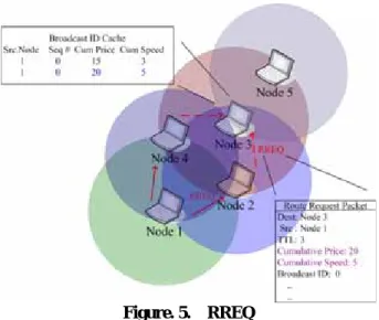
(5) 5: AD HOC ON DEMAND PRICING ROUTING PROTOCOL There are many routing protocols for mobile ad hoc networks. We choose to modify ad hoc on demand distance vector routing protocol. We combine pricing mechanism and AODV routing algorithm into a new one：ad hoc on demand pricing routing protocol（AOP）. We extend the AODV to further include cumulative price and cumulative speed in the Broadcast ID Cache. They are separately the sum of node’s link price and speed. AOP builds routes using a route request / route reply query cycle. When a source node desires a route to a destination for which it does not already have a route, it broadcasts a route request (RREQ) packet across the network. Nodes receiving this packet update their information for the source node and set up backwards pointers to the source node in the route tables. In addition to the source node's IP address, current sequence number, and broadcast ID, the RREQ also contains the most recent sequence number for the destination of which the source node is aware. A node receiving the RREQ may send a route reply (RREP) if it is the destination. If this is the case, it unicasts a RREP back to the source. Otherwise, it rebroadcasts the RREQ. Nodes keep track of the RREQ's source IP address and broadcast ID. If they receive a RREQ which they have already processed, they check if this path is an efficient routing path. We take an example in Figure. 5. Node 3 receives RREQ which has the same source node and sequence number. One’s cumulative price is higher than the other but its expected connection time is less. So the second RREQ is not an efficient routing path and node 3 just drops it.. 6: SIMULATION MODEL AND RESULTS ANALYSIS We show the simulation results in this section. We evaluate the AOP through simulations by using the Network Simulation Version 2 (NS-2)[9].. 6.1: SCENARIO DESCRIPTION The setdest tool in ns2 is used to generate the random topologies for the simulations. Mobility models were created for the simulations using 25 nodes, with pause times of 0, 20, 40, 60, 80, 100 seconds, maximum speed of 20m/s, topology boundary of 1000x1000 and simulation time of 100secs. For the simulations carried out, traffic models were generated for 25 nodes with cbr traffic sources. The packet size is 512 bytes, and the sending rate is 512 Kbps.. Figure. 5. RREQ. 6.2: PERFORMANCE METRICS The performance of AOP is evaluated and compared against AODV, DSDV, and DSR for the network scenarios outlined above. To evaluate the performance, we use the following metrics： z Packet delivery fraction — The ratio of the data packets delivered to the destinations to those generated by the CBR sources. z Average end-to-end delay of data packets — This includes all possible delays caused by buffering during route discovery latency, queuing at the interface queue, retransmission delays at the MAC, and propagation and transfer times. z Efficiency — The ratio of the packet delivery fraction to the payment. This value is the metric of one unit price can transfer successfully how many packets.. 6.3: SIMULATION RESULTS In this section, we present the simulation results and analysis. AOP-T is the method which chooses the longest expected connection time from efficient routing paths. AOP-P is the method which chooses the lowest price from efficient routing paths. From figure 6 we can find that on-demand routing protocols delivery over 70% of the data packets regardless of mobility rate, and outperform the table-driven routing protocol, DSDV. Figure 7 shows the average end to end delay. The average end-to-end delay of packet delivery is lower in AOP-T and AOP-P as compared to other on-demand routing protocols. From figure 8 we can find AOP-T and AOP-P are more efficient than other routing protocols. Using AOP routing protocol, users can transfer packets with the less payment.. - 644 -.

(6) The simulation results bring out some important characteristic differences between the routing protocols. The presence of high mobility implies frequent link failures and each routing protocol reacts differently during link failures. The different basic working mechanisms of these protocols lead to the differences in the performance. The results show that our routing protocols (AOP-T and AOP-P) outperform than other routing protocols. Although the packet delivery of AOP is almost the same with others, the end-to-end delay is lower and the efficiency is highest.. 100 90 packet delivery ratio(%). 80 70 60 50 40 30 20 10. 7: CONCLUSIONS AND FUTURE WORK. 0 0. 20. 40. 60. 80. 100. DSDV. DSR. mobile time(secs) AOP-T. AOP-P. Figure. 6.. AODV. The packet delivery ratio. 0.018 0.016. In this paper we proposed a pricing mechanism based on currency exchange network in MANET. We also indicate how to choose an efficient routing path considering user mobility. Besides, we propose a routing protocol based on pricing mechanism. The results show that our algorithms improve network performance and efficiency. In the future, how to integrate user’s utility function with our routing path selection may be another issue we will concern.. average delay (secs). 0.014 0.012. 8: REFERENCCES. 0.01. [1]. 0.008 0.006 0.004. [2]. 0.002 0 0. 20. 40. 60. 80. 100. [3]. mobile time (secs) AOP-T. PDR * 100 / payment. Figure. 7.. AOP-P. AODV. DSDV. DSR. [4]. The average end-to-end delay. 10 9 8 7 6 5 4 3 2 1 0. [5] [6]. [7] [8] 0. 20. 40. 60. 80. 100. Mobile time (secs) AOP-T. AOP-P. Figure. 8.. AODV. [9] DSDV. DSR. Efficiency. - 645 -. Buttyan, L. and Hubaux, J.P., August 2000, “Enforcing Service Availability in Mobile Ad-Hoc WANs” Proceedings of IEEE/ACM Workshop on Mobile Ad Hoc Networking and Computing Buttyan, L. and Hubaux, J.P., January 2001, “Nuglets: a Virtual Currency to Stimulate Cooperation in Self Organized Mobile Ad Hoc Networks” Technical Report EPFL Buttyan, L. and Hubaux, J.P., October 2003, “Stimulating Cooperation in Self-organizing Mobile Ad Hoc Networks” ACM/Kluwer Mobile Networks and Applications, vol. 8, no. 5, pp.579-592, October 2003 Crowcroft, J., Gibbens, R., Kelly, F., and Ostring, S., March 2003 " Modelling incentives for collaboration in Mobile Ad Hoc Networks", Proceedings of Modeling and Optimization in Mobile, Ad Hoc and Wireless Networks (WiOpt) Zhong, S., Yang, R., Chen, J., March 2003, “Sprite : A Simple, Cheat- Proof, Credit-Based System for Mobile Ad-hoc Networks” Proceedings of INFOCOM 2003 Kai Chen, Klara Nahrstedt, “iPass: an Incentive Compatible Auction Scheme to Enable Packet Forwarding Service in MANET”, in Proc. of 24th IEEE International Conference Marti, S., Giuli, T.J., Lai, K., and Baker, M., 2000 “Mitigating routing misbehaviour in mobile ad hoc networks” Proceedings of MOBICOM 2000. Y. Qiu and P. Marbach, “Bandwith Allocation in Ad-Hoc Networks: A Price-Based Approach,” in Proc. of INFOCOM, 2003 http://www.isi.edu/nsnam/ns/.

(7)