Constructing an Ontology Automatically by Projective ART Neural Network

全文

(1)Constructing an Ontology Automatically by Projective ART Neural Network. 1. Rung-Ching Chen1, Cheng-Han Chuang1, Chiu-Che Tseng2 Chaoyang University of Technology,Department of Information Management, Taichung County, Taiwan, Republic of China [email protected] 2 Texas A&M University-Commerce Department of Computer Science and Information Systems Commerce, Texas 75429 [email protected] ABSTRACT. Ontology is playing an important role in Semantic Web, biomedical informatics and knowledge management. At the same time, constructing and maintaining ontology has become challenges in efficiency and accuracy. In this study, we present a novel ontology construction based on artificial neural network and Bayesian network. First, we collected the web pages related to the problem domain. Then utilize the labels from the HTML tags to selected keywords and utilize WordNet to determine the meaningful keywords called terms. Next, calculate Entropy value to determine the weight of terms. After above steps, using a projective adaptive resonance theory neural network(PART) clusters the terms. Finally, the system outputs an ontology using Bayesian network to express the hierarchical relation among the keywords. Keywords: Ontology, WordNet, Entropy, PART, Bayesian network. 1: INTRODUCTIONS Ontology is playing a more important role in semantic web, biomedical informatics and knowledge management. Semantic web was presented by W3C[1] and made machine-readable information become machine-understandable information. Ontology is the core technology of semantic web. The expansion of semantic web and its success or not depended on whether ontology can be constructed fast and efficiently. The ontology research of biomedical informatics is becoming widespread in recent years. The development of ontology in biomedical informatics is called gene ontology(GO)[2]. The purpose of GO is to deal with the complex information in medicine and to bridge the gap that exists between medical application and basic biological research[3]. In knowledge management, ontology plays a role of supplying and storing information[4]. Combining with Web mining, the ontology will supply the most correct information that users wanted. More recently, the exponential increases. in web sites and biological data have led to an awareness of the usefulness of ontology construction. Traditional ontology construction leans on domain experts but it is costly, lengthy and arguable[5]. There are a lot of ontology construction tools are available, like OntoTrack[6], OntoSeek[7], OntoEdit[8], but ontology construction still needs human effort. We generalize the three major lack[9][10] in ontology and expatiate below: 1.1: LACK OF STANDARD TO REUSE OR INTEGRATE EXISTING ONTOLOGY Ontology is a new and developing technology. There have some organizations such as IEEE working group, Stanford University to create standards for ontologies. Standardization can be divided in three layers: methodology layer, language layer and content layer. The ontology language includes XOL, SHOE, OML, RDF, RDF Schema, DAML+OIL. Owing to the variety of ontology language, the integration of existing ontology is very hard. The reuse of ontology can not be achieved due to the integration of ontology is difficult.. LACK OF METHOD IN FULL AUTOMATIC KNOWLEDGE ACQUISITION 1.2:. Ontology construction is a time and cost consuming procedure. In system such as OntoTrack[6], large amount of knowledge must be defines into the ontology manually first and the system then utilizes the knowledge and creates the full ontology. Using automatic knowledge retrieval methods and tools reduces the time and cost of the ontology construction.. THE LACK OF FLEXIBILITY CLUSTER. 1.3:. IN. Using manual classification framework is the best way to understand what the web pages really mean. But due to the web pages rapidly increase and obsolete, the manual classification framework is hard to catch up the. - 1487 -.

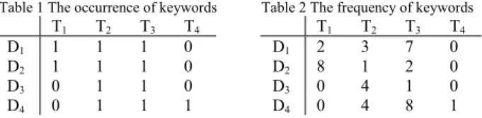
(2) dynamic changes of web pages. Although the current ontology construction methods can achieve a partially automated classification framework, there are still several limitations. At present, the task of making a significant breakthrough and achieves a fully automated classification framework is under investigation. In order to overcome above lack, we proposed a novel method consists of PART neural network and Bayesian network to construct ontology automatically. The system picked web documents from a specific domain, and it carries on the analysis of web pages to choose relevant keywords by WordNet. The candidate keywords(terms) are extracted by calculating Entropy value. Next, we are according to terms to construct a two-dimension matrix with documents and terms for PART neural network to cluster the keywords. Finally, using Bayesian Networks to express the hierarchical relation of terms and construct full ontology. The remainder of the paper is organized as follows. Section 2 introduces the Projective ART neural network and why do we choose the PART to do cluster. In Section 3, we propose how to automatically generate an ontology. Section 4 specifies the experiment results. Finally, the paper makes conclusions and future work in Section 5.. approach based on a new neural network architecture – PART(Projective Adaptive Resonance Theory) in 2002[12]. The basic architecture of PART is similar to the ART neural networks. The main difference between PART and ART is in the input layer. In PART, the input layer selectively sends signals to nodes in the output layer(cluster layer). The signals are determined by a similarity check between the corresponding top-down weight and the signal generated in the input layer. Hence, the similarity check plays a crucial role in the projected clustering of PART. Besides the vigilance test, the PART adds the distance test to increase the accuracy of clustering. Fig. 1 illustrates the basic PART architecture and the PART algorithm is presented below. Table 3 shows the definition of parameters appeared in the PART algorithm. output layer Y1. W11b. X1. 2.1: PROJECTIVE ADAPTIVE RESONANCE THEORY Adaptive resonance theory(ART) neural network is an unsupervised learning network proposed by S. Grossberg in 1976[11]. The ART has both features of stability and plasticity. In the initial study, we adopt the ART to cluster concepts. Every pattern was presented by whether the keywords appear on web pages or not. Unfortunately, the above method will bring the problems of feasibility and reliability. In ART neural network, input vectors is constituted by {0, 1}. However, there were not all of data sets in our study were picked up in the two values. Therefore, it is not reliable to present the multi-values data sets by two values. Besides, it is not feasible to cluster such data sets. For example, there are four keywords appear on four documents shows in Table 1. Clustering the four documents by ART, the D1 and D2 will be a cluster. Table 2 shows the frequency of keywords in documents. Obviously, D1 emphasized T3 and T2 should be clustered with D4.. D1 D2 D3 D4. T1 1 1 0 0. T2 1 1 1 1. T3 1 1 1 1. T4 0 0 0 1. Table 2 The frequency of keywords. D1 D2 D3 D4. T1 2 8 0 0. T2 3 1 4 4. T3 7 2 1 8. T4 0 0 0 1. In order to deal with the feasibility-reliability dilemma in clustering data sets of high dimension, Yongqiang Cao and Jianhong Wu presented an. Vigilance and Distance. hij. 2: THE KERNEL TECHNOLOGY. Table 1 The occurrence of keywords. W11t. Similarity Check X2. Xi. Input layer. Fig. 1 The architecture of PART Table 3 The list of PART parameters Parameter Wij Wji σ θ ρ L n α. Meaning Bottom-up weight Top-down weight Distance parameter Threshold Vigilance parameter Constant parameter Pattern amount Learning rate. Permissible range NA NA NA 0＜θ≦n 1≦ρ≦n L≧1 NA 0≦α≦1. PART algorithm 0. Initialization: Initialize parameters L, ρ, σ, α, θ. Input vectors: Xi. Output nodes: Yj. Set Yj has not learned any input pattern. 1. Input the pattern X1,X2,…,Xi. 2. Similarity Check: hij=h(Xi, Wij, Wji)=hσ(Xi, Wji)l(Wij) ⎧1, if d(a, b) ≤ σ Where hσ(a, b) = ⎨ ⎩0, if d(a, b) > σ. ⎧1 , if Wij > θ l(Wij) = ⎨ ⎩0 , if Wij ≤ θ If hij=1, Xi is similar to Yj. Else hij=0, Xi is not similar to Yj. 3. Selection of winner node: Tj=ΣWijhij=ΣWijh(Xi, Wij, Wji) Max {Tj} is the winner node.. - 1488 -.

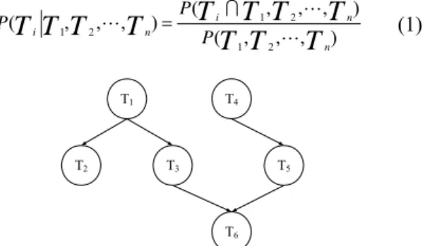
(3) Vigilance and Reset: Rj = Σhij < ρ If the winner node succeeds in vigilance test, the input pattern will be clustered in the winner node. Else, the input pattern will be clustered in a new node. 5. Learning: Update the bottom-up and top-down weights for winner node Yj. If Yj has not learned any pattern before: new Wij = L/(L-1+n) new Wji = Xi If Yj has learned some patterns before: new ⎧L/(L - 1+ | X |), if h = 1 Wij = ⎨ if h = 0 ⎩0,. 4.. ij. ij. new. 6.. old. Wji = (1-α)Wji +αXi Repeat step 2n times, until the number of data points in each cluster falls below the threshold.. 2.2: BAYESIAN NETWORK Bayesian Networks(BN)[13] is a popular framework for reasoning under uncertainty. A Bayesian Network can be divided into two main part, B = (G , Θ). The first part G is a directed acyclic graph(DAG) consisting of nodes and arcs. The nodes are the variables T = {T1,T2….Tn} in the data set whereas the arc indicates direct dependencies between the variables. The second part of Bayesian Network Θ represents the conditional probability distributions, and is stored in a conditional probability table(CPT). Then, Bayesian Networks can be represented as the following joint probability distribution: P (T i T 1,T 2 ,L ,T n ) =. T1. T2. P (T i I T 1 ,T 2 ,L,T n ) P (T 1 ,T 2 ,L,T n). model. Such probabilities are not directly stored in the network; hence, it is necessary to calculate them. In general, given a network, the calculation of a probability of interest is well known as probabilistic inference, and is usually based on Bayes’ theorem. In the case of problems with many variables, the direct approach is often not practical. Nevertheless, at least when all the variables are discrete, we can expand the conditional independences encoded in a Bayesian network so as to make the calculation more efficient. In this paper, we use Bayesian Network to construct ontology because there are several advantages for data analysis in Bayesian Networks. First, BN encodes dependencies within all variables, so it can deal with missing data entries easily. Secondly, the network can be used to handle causal relationships and hence it can be used to gain understanding about a problem domain and to predict results. Third, BN is a technology based on statistics which offers a valid and widely recognized approach for avoiding the over-fitting of data. Finally, the diagnostic performance with the Bayesian Network is often surprisingly insensitive to imprecision in the numerical probabilities.. 3: RESEARCH METHODOLOGY The presented system can be divided into two main subsystems: term parsing and ontology construction subsystem. The system architecture shows in Fig. 3. Both the subsystems are described in the following subsection:. (1). T4. T3. T5. T6. Fig. 2 A simple of Bayesian Networks where each variable is independent of its non-descendants given its parents in the graph. For example in Fig. 2, we want to calculate the conditional probability of P(T6). According to the formula(1), the conditional probability will be P(T6∣T1, T2, T3, T4, T5). In Fig. 2, the paternal nodes of T6 were merely T3 and T5 and we will obtain P(T6∣T1, T2, T3, T4, T5) = P(T6∣T3, T5). Based on the characteristic of Bayesian network, P(T6∣T3, T5) = P((T6∩T3)P(T6∩T5))/P(T3, T5). Once the Bayesian network is constructed (through a prior probability or from data), it is imperative to determine the various probabilities of interest from the. Fig. 3. The system architecture. 3.1: TERM PARSING SYSTEM 3.1.1: WEB PAGES ANALYSIS. We utilized the characteristic of URL(Universal Resource Locator) to collect web pages from Internet, and analysis the keywords in the domain. Each of the domain keywords need to be found at least one time in. - 1489 -.

(4) one of the web pages. Otherwise, we will delete the web page. We then adopt WordNet[14] developed by Princeton University to ascertain the existence of keywords. WordNet is an online lexical reference system. English nouns, verbs, adjectives and adverbs are organized into synonym sets, each representing one underlying lexical concept. Different relations link the synonym sets. We also consider the problem of stop word within the web pages. Finally, we output the preliminary relationship between keywords and web pages for the next step of analysis.. choose the highest entropy value in the every cluster to represent the cluster.. 2 2 2 2 5 5 3 3. 3.1.2: ENTROPY. The entropy[15] can be applied to analyze page content blocks and discover informative content. We use Shannon’s information entropy to calculate the keyword entropy based on keyword-WebPages matrix that obtained form above step. The matrix stored the frequency of keywords appear in documents. The entropy E can be normalized the feature of a feature to be [0, 1], the entropy formula of keyword Ti is: E (T ) = −∑ P m. i. j =1. ij. log. P. ij. (2). m. where m is the set of web pages, and Pij means the probability that the keyword i appears in web page j. After calculating, we delete the keywords whose entropy value is 0. The remainder terms will use to construct the final ontology.. 3.2: ONTOLOGY CONSTRUCTION SYSTEM. Table 4 A sample of TF-matrix T2 3 3 3 3 4 4 4 4. T3 4 4 2 2 3 3 3 3. 0 7 8 2 3 7 4 7. 4 4 2 2. 0 7 8 2. 5 5 3 3. 4 4 4 4. 3 3 3 3. 3 7 4 7. 2 3 4 0 2 3 4 7. 2 3 2 8 2 3 2 2 5 4 3 3 5 4 3 7. 3 4 3 4 3 4 3 7. 3.2.2: APPLICATION OF BAYESIAN NETWORK.. After the PART tree process, we got a basic tree structure that can be used to represent whole web pages. We used Bayesian Network to construct the complete domain ontology. The system calculated the condition probability of all terms and store the probability in CPT. Then insert the terms one by one by comparing the condition probability with entropy value between terms. Repeating the steps, we can build a DAG to represent the domain ontology. For example, we obtained n candidate keywords T1,T2,…,Tn from the above steps. Then we calculated the condition probability based on prior probability P(T1), P(T2), … ,P(Tn) and store the values in CPT, showed in Table 5. Table 5 The conditional probability of terms. After above steps, we can get a term-document matrix call TF-matrix. The TF-matrix is inputted to PART. In order to obtain the PART tree architecture, we add the recursion to the PART architecture. We believe that the PART tree will provide more information about the hierarchical relation of projective clusters[16]. Take Table 4 for example, there is a data set of eight patterns. We utilize PART to cluster the data set, where ρ=1, σ=0.1, L=2, α=0.1, θ=1. T1 2 2 2 2 5 5 3 3. 4 4 2 2 3 3 3 3. 3 3 3 3. Fig. 4 The tree of sample. 3.2.1: APPLICATION OF PROJECTIVE ART. D1 D2 D3 D4 D5 D6 D7 D8. 3 3 3 3 4 4 4 4. 2 2 2 2. T4 0 7 8 2 3 7 4 7. According to the recursive feature, we will obtain the tree of Table 4 shows in Fig. 4. We divide the cluster recursively by the same way based on a threshold value. If it is lower than the threshold value, it will not cluster again. We then. T1 T2. T1 null P(T1|T2). T2 P(T2|T1) null. … … …. Tn P(Tn|T1) P(Tn|T2). …. …. …. …. …. Tn. P(T1|Tn). P(T2|Tn). …. null. The columns represent prior probability and the rows represent the inference condition probability. We determine the order of inference based on entropy value. Assume that T1, T2, T3, T4 are the node of the basic tree structure. T5 has the higher entropy value than the remainder terms. We inserted T5 to the DAG, and checked CPT based on the prior probability of T1, T2, T3, T4. Assuming that T3 inferred to T5 has the highest condition probability. We knew that T5 must be the descendants of T3. Following these steps, we can build the domain DAG and the DAG is the domain ontology. 3.2.3: ONTOLOGY EXPRESSION. In section 1.1, we referred that there are a lot of ontology languages so that the integration of existing ontology is very hard. This system finally output an ontology using RDF format through a package of Jena.. - 1490 -.

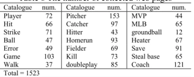
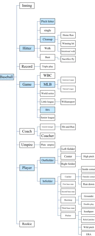
(5) The RDF(Resource Description Framework) is a general-purpose language for representing information in the Web. The RDF can help integration and reuse of exiting ontology[17].. must be the descendant of node player. That is because the web pages recently always refer drugs and Barry Bonds at the same time. That is the influence of the partial data in small sample. Table 7 Ontology results of the first stage. 4: EXPERIMENT AND DISCUSSION In our experiments, the data sources are collected from the catalogue that has already been classified separately by Google[18] and ESPN[19]. We select the domain of baseball as our problem domain for the experiments. Table 6 shows the domain with 21 catalogues. If the web pages do not include any concepts in their catalogue, they will be removed. For example, web pages in the ”Catcher” catalogue must include at least one keyword ”Catcher”. After pre-processed the 2400 web pages, we obtained 1523 web pages as our domain data.. Num. of documents Num. of keywords Num. of terms Depth of ontology Breadth of ontology Precision Recall. In the second stage, we repeat the above steps and the detail of the ontology are showed in Table 8. We discover that the results are better accompanying the data increased. Table 8 Ontology results of the second stage Num. of documents Num. of keywords Num. of terms Depth of ontology Breadth of ontology Precision Recall. Table 6 The number of collected web pages Catalogue Player Hit Strike Ball Error Game Walk Total = 1523. num. 72 66 71 47 49 103 37. Catalogue Pitcher Catcher Hitter Homerun Fielder Kill doubleplay. num. 153 97 43 93 69 73 85. Catalogue MVP MLB groundball Heater Save Steal base Coach. num. 44 65 12 67 91 65 121. Afterward, we want to know whether the quantity of data will influence the result or not. We divide the experiment to the three stages and the study adopts the precision and recall to evaluate the ontology result. In the first stage, we extract 30% of the 1523 web pages about 457 web pages randomly. In the second stage, we extract 914 web pages about 60% of total web pages. In the third stage, the total web pages are included. The each experiment is clustered by PART, where L=2, ρ=3, σ=0.4, α=0.1, θ=4. Precision =. Recall =. | relevant | ∩ | retrieved | | retrieved |. | relevant | ∩ | retrieved | | relevant |. 914 72 41 4 10 73.1%(11) 70.7%(12). In the third stage, we inputted the total web pages to the system. Although the compute of experiment was increasing, the accuracy of final ontology was increasing relatively. Table 9 shows the detailed ontology of the third stage. The diagram of final ontology in the third stage is showed in Fig. 5 and stored the ontology by RDF in computer. In the Fig. 5, the blue nodes stand for the clustering result of PART. For example, the terms were clustered into three groups and the system picked the nodes Hitter, Game, Player to present the group respectively. The each group will be clustered continuously. The dotted nodes stand for the incorrect node that domain experts determined. Table 9 Ontology results of the third stage. (3). Num. of documents Num. of keywords Num. of terms Depth of ontology Breadth of ontology Precision Recall. (4). The three data sets are inputted to the system respectively. The first stage got 46 keywords from the web pages analysis and WordNet. After calculating the entropy value, we obtained 27 terms to cluster. Through the PART tree architecture, the system generated a basic tree of three nodes. Finally, the system inserted the remainder terms by Bayesian network. The detail of the ontology is showed in Table 7. We find the results of the first stage are not good enough. The system is based on the inference of probability. It is possible that the result will be influenced by the partial data especially the small sample. For example, we discover the node drugs in the ontology of the first stage has a descendant node Bonds(a MLB player). In fact, the node Bonds. 457 46 27 3 14 65.4%(10) 59.2%(11). 1523 79 53 5 8 84.9%(8) 75.4%(13). 5: CONCLUSION AND FUTURE WORK In the study, we presented an automatic ontology construction based on projective ART and Bayesian network. The PART architecture overcomes the lack of flexibility in clustering. The web pages analysis, WordNet and Entropy deal with the lack of knowledge acquisition. The final RDF will hasten the integration and reuse of exiting ontology. Besides, the experiment shows the better result than the average. In the future works, we plan to reduce the compute of Bayesian network. Furthermore, we would like to explore well defined criteria to evaluate our system. - 1491 -.

(6) performance. Finally, the system proposed here is only constructed in one particular domain. We will attempt to combine with multi-field ontology to develop a well rounded system.. [2]. [3]. Inning. [4] Pitch hitter. [5]. single Home Run. Cleanup Winning hit. Hitter. Walk Bunt. Record. [6]. Intentional walk. Sacrifice fly. Triple play. [7]. WBC. Baseball. American League. Game. [8]. MLB National League. World series Little league. Williamsport. [9]. IBA Senior league. General manager. Hit-and-Run. [10]. Coach Coacher Umpire. Plate umpire. [11]. Left fielder Center. High pitch. Outfielder Right fielder. Player. Inside corner Catcher. Outside corner. First base man. Run down. Infielder. [12]. [13]. Second base man. Grounder Shortstop Double play Third base man. Southpaw. [14] [15]. Pitcher Relief pitcher. Rookie Wild pitch ERA. Fig. 5 Ontology diagram of the third stage. REFERENCES [1]. [16]. [17]. W3C, http://www.w3.org [18] [19]. - 1492 -. C. Blaschke, A. Valencia, “Automatic Ontology Construction from the Literature,” Genome Informatics, vol. 13, pp. 201-213, 2002. A. C. Yu, “Methods in biomedical ontology,” Journal of Biomedical Informatics, vol. 39, pp. 252-266, 2006. Y. Li, N. Zhong, “Mining Ontology for Automatically Acquiring Web User Information Needs,” IEEE Transactions on Knowledge and Data Engineering, vol. 18, no. 4, 2006. R. Navigli, P. Velardi, A. Gangemi, “Ontology Learning and Its Application to Automated Terminology translation,” IEEE Intelligent System, vol. 18, no. 1, pp. 22-31, 2003. T. Liebig, O. Noppens, “ONTOTRACK: A Semantic approach for Ontology Authoring,” Web Semantics: Science, Services and Agents on the World Wide Web, vol. 3, pp. 116-131, 2005. N. Guarino, C. Masolo, G. Vetere, “OntoSeek: Content-based Access to the Web,” IEEE Intelligent Systems, vol. 14, no. 3, pp. 70-90, 1999. Y. Sure, M. Erdmann, J. Angele, S. Staab, R. Stider, D. Wenke, “OntoEdit: Collaborative Ontology Development for the Semantic Web,” Proceedings of the First International Semantic Web Conference, 2002. S. S. Weng, H. J. Tsai, S. C. Liu, C. H. Hsu, “Ontology Construction for Information Classification,” Expert Systems with Application, vol. 31, pp. 1-12, 2006. M. Shamsfard, A. A. Barforoush, “Learning Ontology from Natural Language Texts,” Int. J. Human-Computer Studies, vol. 60, pp. 17-63, 2004. G. A. Carpenter, S. Grossberg, “The ART of Adaptive Pattern Recognition by Self-Organizing Neural Network,” Computer Science, vol. 22, no. 3, pp. 77-88, 1988. Y. Cao, J. Wu, “Dynamics of Projective Adaptive Resonance Theory Model: The Foundation of PART Algorithm,” IEEE Transactions on Neural Networks, vol. 15, no. 2, pp. 245-260, 2004. L. Denoyer, P. Gallinari, “Bayesian Network Model for Semi-structured Document Classification,” Information Processing and Management, vol. 40, pp. 807-827, 2004. WordNet, http://wordnet.princeton.edu/ H. Y. Kao, S. H. Lin, J. M. Ho, M. S. Chen, “Mining Web Informative Structures and Contents Based on Entropy Analysis,” IEEE Transactions on Knowledge and Data Engineering, vol. 16, no. 1, pp. 41-55, 2004. Y. Cao, J. Wu, “Projective ART for Clustering Data Sets in High Dimensional Spaces,” Neural Networks, vol. 15, pp. 105-120, 2002. G. klyne, J. Carroll, “Resource Description Framework(RDF) Concepts and Abstract Syntax,” W3C Recommendation, 2004. Google, http://www.google.com ESPN, http://espn.go.com.

(7)