國立交通大學
電子工程學系 電子研究所
碩 士 論 文
應用於數位微流體生物晶片中達到反應物及
廢液最小化之多目標濃度樣本製備程序
Reactant and Waste Minimization
in Multi-Target Sample Preparation
on Digital Microfluidic Biochips
研 究 生:林惠珊
指導教授:黃俊達 博士
應用於數位微流體生物晶片中達到反應物及
廢液最小化之多目標濃度樣本製備程序
Reactant and Waste Minimization
in Multi-Target Sample Preparation
on Digital Microfluidic Biochips
研 究 生:林惠珊
Student: Huei-Shan Lin
指導教授:黃俊達 博士
Advisor: Dr. Juinn-Dar Huang
國立交通大學
電子工程學系 電子研究所
碩士論文
A Thesis
Submitted to Department of Electronics Engineering & Institute of Electronics College of Electrical & Computer Engineering
National Chiao Tung University in Partial Fulfillment of the Requirements
for the Degree of Master
in
Electronics Engineering & Institute of Electronics
December 2012
Hsinchu, Taiwan, Republic of China
i
應用於數位微流體生物晶片中達到反應物及
廢液最小化之多目標濃度樣本製備程序
研究生:林惠珊 指導教授:黃俊達 博士 國立交通大學 電子工程學系 電子研究所碩士班摘 要
樣本製備程序(sample preparation)為各種生化反應中不可或缺的步驟。原始生物樣 本或反應試劑必須在此程序中進行稀釋或混合,以達到反應所需的目標濃度(target concentration)。一般來說,一個生化反應通常需要某一樣本的多重目標濃度。但是,大 部分現有的樣本製備程序規劃相關演算法,都是針對單一目標濃度的製備而設計。因此, 當需要製備多目標濃度時,會採用依序製備的方式,這種方式被認為較無效率與耗時。 若所需的多目標濃度在此過程中可以同時製備,那麼稀釋/混合反應的次數與反應物的使 用量都可以再降低。本篇論文提出一個廢液回收再利用的演算法,簡稱 WARA,來解 決在數位微流體生物晶片(digital microfluidic biochips, DMFBs)上,多目標濃度樣本製備 程序規劃(multi-target sample preparation)的問題。WARA 的主要概念為,將樣本製備程 序中的副產物-廢液滴回收後再利用。藉由這個概念,反應物的使用量與廢液滴的生成 量都可以大幅降低。實作上,WARA 透過液滴共享與液滴置換的方法來回收廢液。實 驗結果顯示,與現行成效最好的多目標濃度樣本製備程序演算法相比,當目標濃度數目 為十的時候,WARA 產生的廢液數量較其減少了 48%,而所需要的稀釋/混合反應次數 則減少了 37%;當目標濃度數目持續增加,此降低程度更是顯著─最多可減少 97%的廢 液生成量與 73%的稀釋/混和反應次數。ii
Reactant and Waste Minimization
in Multi-Target Sample Preparation
on Digital Microfluidic Biochips
Student: Huei-Shan Lin Advisor: Dr. Juinn-Dar Huang
Department of Electronics Engineering & Institute of Electronics National Chiao Tung University
Abstract
Sample preparation is an essential process in biochemical reactions. Raw reactants are diluted to reach the given target concentrations. Typically, a bioassay may require several different target concentrations of a reactant. However, most of existing algorithms are designed for single-target sample preparation only. When they are applied to prepare multiple target concentrations, these target concentrations are prepared separately one by one, which is inefficient and time-consuming. If all these target concentrations are produced simultaneously during sample preparation, both the dilution operation count and the reactant usage can be further minimized. In this thesis, we propose a waste recycling algorithm, WARA, to tackle the multi-target sample preparation problem on digital microfluidic biochips (DMFBs). The main idea of WARA is to recycle waste droplets in the dilution process and turn them into usable ones for reactant and waste minimization. WARA achieves waste recycling through droplet sharing and droplet replacement. Experimental results show that WARA can reduce the waste and operation count by 48% and 37% respectively as compared to an existing state-of-the-art multi-target sample preparation method when the number of target concentrations is ten. The reduction can be up to 97% and 73% when the number of target concentrations goes even higher.
iii
誌 謝
特地將致謝留在最後,想要仔仔細細地寫。但是當我終於要下筆了,才發現要感謝 的人好多好多,請原諒我無法一一列舉。 謝謝周景揚教授與張世杰教授擔任我的口試委員,提出寶貴意見,使得此篇論文更 加完整,非常感謝。謝謝黃俊達老師、Terry學長,那些每次的仔細討論、精闢的見解、 投稿前的日以繼夜、百忙之中的抽空、適時的鼓勵加油,謝謝。謝謝實驗室的學長姐、 同學、學弟、BTFT,那些適時的教導、伸出援手、作伴,謝謝。 謝謝我的朋友,那些偶爾的互相關心、沮喪時的打氣電話、一起相聚的約定、遠從 西子灣來的晴天與好心情,那些把我放在心上的人們,謝謝你們。 謝謝我的大寶,在我身邊陪伴,那些等我在實驗室做完事情的日子、傷心難過挫折 生氣時的安慰包容、要一起畢業的希望,我晚了一些,但終於完成了。 謝謝我的家人,在我背後無聲的支持,那些每次回家必定會的加菜、我要回家就抽 空回去相聚的周末、吵鬧嘻笑的飯後家常,那些放在心裡沒說出口的話,我很愛你們, 謝謝。 每結束一個階段,接著必再開啟另一個全新的階段, 謹以此篇論文,獻給大家。 謝謝你們、祝福你們 林惠珊 中華民國一Ο一年十二月iv
Contents
摘 要 ...i Abstract ... ii 誌 謝 ... iii Contents ...ivList of Tables ...vi
List of Figures ... vii
Chapter 1 Introduction ... 1
Chapter 2 Sample Preparation ... 5
2.1 Dilution Procedures ... 5
2.2 Mixing Models ... 6
2.3 Exponential and Interpolated Dilution ... 7
Chapter 3 Previous Works ... 8
3.1 Single-Target Sample Preparation Algorithms... 8
3.1.1 BS ... 8
3.1.2 DMRW and IDMA ... 9
3.1.3 REMIA ... 11
3.2 Multi-Target Sample Preparation Algorithm ... 13
Chapter 4 Problem Description ... 16
4.1 Mixing Tree ... 16
4.2 Motivation ... 20
4.3 Problem Formulation ... 22
Chapter 5 Proposed Algorithm ... 23
5.1 Algorithm Overview ... 23
5.2 Tree Generation ... 24
5.3 Droplet Sharing ... 25
5.4 Droplet Replacement ... 28
Chapter 6 Experimental Results ... 34
v
6.2 Results and Analyses ... 35
6.2.1 Three Consecutive Optimization Phases ... 35
6.2.2 Sample Preparation with Different Tree Generation Techniques ... 38
Chapter 7 Conclusion ... 41
vi
List of Tables
vii
List of Figures
Figure 1. Digital Microfluidic Biochip. ... 1
Figure 2. Electrowetting-on-dielectrics (EWOD) effect. ... 2
Figure 3. The serial dilution process. ... 5
Figure 4. Exponential and Interpolated Dilution. ... 7
Figure 5. A dilution process using BS. ... 8
Figure 6. A dilution process using DMRW. ... 9
Figure 7. A dilution process using IDMA. ... 10
Figure 8. A dilution process using REMIA. ... 11
Figure 9. An initial dilution graph produced by IDSA. ... 13
Figure 10. The dilution graph produced by IDSA after combining intermediate nodes. ... 14
Figure 11. The dilution graph produced by IDSA after utilizing intermediate nodes. ... 15
Figure 12. Two mixing trees produced by REMIA. ... 17
Figure 13. Reactant-minimal exponential dilution process for Figure 12. ... 18
Figure 14. Optimal unified exponential dilution process (OUED). ... 19
Figure 15. A motivational example of droplet sharing. ... 20
Figure 16. A motivational example of droplet replacement. ... 21
Figure 17. The overall algorithm flow of WARA. ... 23
Figure 18. Tree generation... 24
Figure 19. Droplet sharing. ... 26
Figure 20. The pseudo code of droplet sharing. ... 27
Figure 21. Droplet Replacement. ... 28
Figure 22. Droplet replacement is order dependent. ... 29
Figure 23. An additional PCV node is allowed while creating an RCP. ... 30
Figure 24. The tie-breaking score (uniqueness) for droplet replacement. ... 30
Figure 25. An example of droplet replacement. ... 32
Figure 26. The pseudo code of droplet replacement. ... 33
Figure 27. The experimental flow. ... 35
Figure 28. The reactant/buffer/waste/operation count per target for various #Ct. ... 37
viii
Chapter 1 Introduction
Lab-on-a-chip (LoC), a kind of biochip, is one of the most popular research topics in recent years [1]. An LoC is an analysis system that integrates many biochemical functions in a small chip, such as injection, mixing, separation, and detection [2]. Compared with conventional biochemical systems in labs, hospitals, or research centers, which are always bulky and expensive, LoCs offer many advantages like portability, reagent volume reduction, automation, mass production, fast analysis, high throughput, and low power consumption [3].
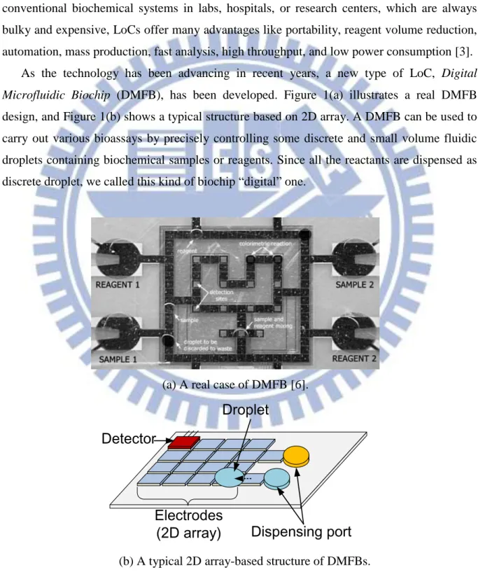
As the technology has been advancing in recent years, a new type of LoC, Digital Microfluidic Biochip (DMFB), has been developed. Figure 1(a) illustrates a real DMFB design, and Figure 1(b) shows a typical structure based on 2D array. A DMFB can be used to carry out various bioassays by precisely controlling some discrete and small volume fluidic droplets containing biochemical samples or reagents. Since all the reactants are dispensed as discrete droplet, we called this kind of biochip “digital” one.
(a) A real case of DMFB [6].
Electrodes
(2D array)
Droplet
Detector
Dispensing port
(b) A typical 2D array-based structure of DMFBs. Figure 1. Digital Microfluidic Biochip.
2
The electrowetting-on-dielectrics (EWOD) effect is utilized as an electrostatic actuation method to dispense, transport, split, merge, and mix droplets on DMFBs. Through applying control voltage on the electrodes below the chip, the surface tension of droplets can be changed. The induced force is used to move these droplets, as shown in Figure 2 [4]–[7]. Therefore, a biochemical assay can be conducted via a series of basic droplet operations.
High voltage
dropelt
(a) Top view.
Glass
Glass
Droplet
High voltage
(b) Side view. Figure 2. Electrowetting-on-dielectrics (EWOD) effect.
Recently, lots of on-chip laboratory procedures, such as immunoassay, protein crystallization, and DNA sequencing, have been successfully demonstrated on DMFBs [8]. Because the demand for various applications continuously grows, the design complexity of DMFBs is certainly increased. Therefore, a series of automation algorithms are necessary for speeding up the process, reducing the manual effort, and improving the design quality. In the past few years, lots of design automation algorithms are proposed to tackle problems in DMFB design flow, such as synthesis, placement, routing, control pin assignment, and chip testing [9]–[20]. Undoubtedly, the design automation for DMFB is one of the most emerging topics nowadays, and the related research works are proliferating.
Sample preparation problem is one of the critical issues in DMFB design automation. Reactants (sample or reagent) must be diluted to the specific concentration, which is called target concentration, in the process. There are some factors may affect the quality of whole dilution process, they are:
(1) Usage of valuable reactants: it is the major cost for a biochemical reaction. The usage of valuable reactant which is very expensive or is limited in amount, like costly reagents or infant’s blood, should be minimized. An analysis would fail if the preparation process does not consider reactant minimization.
(2) Number of waste droplets: since the number of waste reservoirs on a given DMFB is fixed, the capacity for waste handling is accordingly limited. The excessive waste count may lead to long preparation time. Furthermore, keeping too much waste droplets on DMFB is not propitious for droplet routing. That is, it makes the routing more complicated and may require much extra transportation time to drive waste droplets into reservoirs.
(3) Number of dilution operations: it basically represents the preparation time, and thus should be minimized. A long preparation process may be a fatal in some urgent clinical incidents.
Several algorithms which tackle the sample preparation problem on DMFBs have been proposed [24]–[31]. Most of them address on single-target sample preparation. That is, they generate each target CV through an individual dilution process. If multiple target CVs are required, different target concentrations must be produced one-by-one and is thus time-consuming. Moreover, since those methods do not consider reactant sharing among different dilution process, they may lead to higher reactant usage and waste count.
Intermediate droplet sharing algorithm (IDSA) [29] is the first work that deals with the concurrent preparation for multiple target concentrations. It reduces waste amount by means of minimizing the number of intermediate concentrations in dilution process. However, this strategy does not always lead to a better result. Furthermore, in our opinion, minimizing the usage of valuable reactant is as important as waste reduction. Thus, an approach which can achieve both reactant and waste minimization in multi-target sample preparation is necessary.
In this thesis, we propose a waste recycling algorithm (WARA) for multi-target sample preparation on DMFBs. WARA adopts a tree-based dilution strategy. It generates a mixing tree for each target concentration at beginning, and recycles the waste droplets among those trees by droplet sharing and droplet replacement. Experimental results show that WARA reduces the amount of (waste, operations) by (48%, 37%) on average as compared to IDSA if the number of targets is ten1. The reduction can be up to (97%, 73%) as the number of target concentrations grows to 100. The results suggest that WARA should be a better solution for multi-target sample preparation on DMFBs.
The rest of this thesis is organized as follows. Chapter 2 describes the sample preparation process. Chapter 3 briefly introduces previous works. In Chapter 4, we identify our motivation and the problem formulation. Our multi-target sample preparation algorithm,
1 Since IDSA reported its results by means of bar charts, we have done our best to compare
4
WARA, is elaborated in Chapter 5. The experimental results are reported and discussed in Chapter 6. Finally, Chapter 7 concludes this paper.
Chapter 2 Sample Preparation
2.1 Dilution Procedures
The goal of sample preparation is to prepare specific target concentrations (Ct) through a
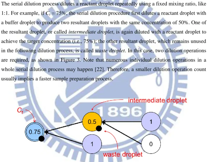
series of dilution operations. On biochips, both linear dilution and serial dilution procedures are commonly used [21][22]. However, the serial dilution is more suitable than the linear one on DMFBs because reactants are dispensed as discrete droplets instead of continuous flows. The serial dilution process dilutes a reactant droplet repeatedly using a fixed mixing ratio, like 1:1. For example, if Ct = 75%, the serial dilution procedure first dilutes a reactant droplet with
a buffer droplet to produce two resultant droplets with the same concentration of 50%. One of the resultant droplet, or called intermediate droplet, is again diluted with a reactant droplet to achieve the target concentration (i.e., 75%); the other resultant droplet, which remains unused in the following dilution process, is called waste droplet. In this case, two dilution operations are required, as shown in Figure 3. Note that numerous individual dilution operations in a whole serial dilution process may happen [22]. Therefore, a smaller dilution operation count usually implies a faster sample preparation process.
6
2.2 Mixing Models
There are different mixing models that can be performed on various DMFB architectures. Three kinds of mixing models are commonly adopted in previous works. Suppose the ratio between two substances for mixing is (x: y), the three mixing models can be expressed as: (1) ; (2) ; (3) . The second model is adopted in previous works [27]–[29] through a special designed rotary mixer. However, the rotary mixer occupies much chip area and is not an essential block of DMFB. For most general DMFBs, only the first mixing model can be easily performed through linear or array mixers [5]. Hence, we adopt the first mixing model, named (1:1) mixing model, in this work, just as the previous works [26][30][31] do. Accordingly, the number of (1:1) dilution operations is then used to estimate the sample preparation time.
However, an inherent error between the target concentration and the value can be achieved may exist no matter which mixing model is adopted. The inherent error is unavoidable if the denominator of the target concentration is not a power of two or even not a rational number, like 3 or √ . Even through, it can be minimized to an acceptable range if the precision level is high enough [26][27]. A precision level n implies that n fractional bits are used to represent the target concentration and the error is limited to accordingly. Users can determine a proper precision level to make this error acceptable.
2.3 Exponential and Interpolated Dilution
Under the (1:1) mixing model, a dilution operation first mixes two source droplets into a mixture and then splits it into two resultant droplets [22]. The two resultant droplets have the same concentration value (CV for short). The relation between these droplets can be expressed as:
(1)
Where C1 and C2 represent the CVs of two source droplets and Cr is the CV of the
resultant droplets.
A dilution operation can be further classified as two types: exponential dilution and interpolated dilution [22]. An exponential dilution is a dilution operation which one of its source droplets is buffer. For example, if a droplet with CV = C is diluted with a buffer droplet, the CV of the resultant droplet is ; if n exponential dilution operations are applied consecutively, the CV of the final two resultant droplets finally becomes . In this thesis, a CV is called a prime concentration value (PCV) if it is equal to 1 or can be produced through a series of exponential dilutions starting from a raw reactant droplet (i.e., CV = 1), for
example, . That is, a PCV contains only one bit ‘1’ in its binary representation. On the
other hand, for an interpolated dilution, neither two source droplets is buffer. Both the two kinds of dilution operations are necessary to prepare an arbitrary target CV. Figure 4 illustrates the two types of dilution processes.
0 1 0 0 0 0 1 2 1 4 1 8 1 16 1 32 ... 0.12 0.012 0.0012 0.00012 0.000012 PCVs ... 1 2n ... 0
(a) Exponential dilution.
C2
C1
C1+C2
2
(b) Interpolated dilution. Figure 4. Exponential and Interpolated Dilution.
8
Chapter 3 Previous Works
3.1 Single-Target Sample Preparation Algorithms
3.1.1 BS
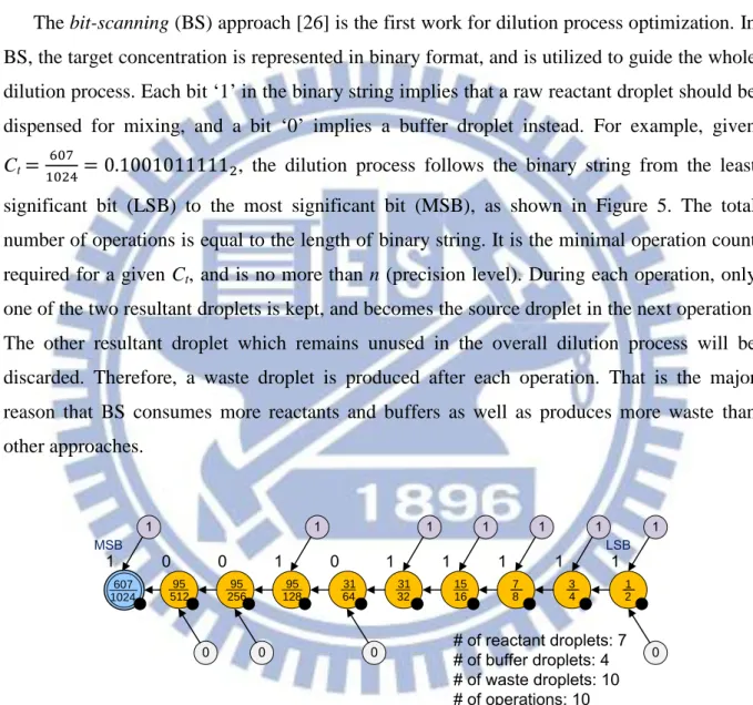
The bit-scanning (BS) approach [26] is the first work for dilution process optimization. In BS, the target concentration is represented in binary format, and is utilized to guide the whole dilution process. Each bit ‘1’ in the binary string implies that a raw reactant droplet should be dispensed for mixing, and a bit ‘0’ implies a buffer droplet instead. For example, given
Ct
, the dilution process follows the binary string from the least significant bit (LSB) to the most significant bit (MSB), as shown in Figure 5. The total number of operations is equal to the length of binary string. It is the minimal operation count required for a given Ct, and is no more than n (precision level). During each operation, only
one of the two resultant droplets is kept, and becomes the source droplet in the next operation. The other resultant droplet which remains unused in the overall dilution process will be discarded. Therefore, a waste droplet is produced after each operation. That is the major reason that BS consumes more reactants and buffers as well as produces more waste than other approaches. 256 95 512 95 128 95 64 31 32 31 16 15 1024 607 8 7 4 3 2 1 0 1 0 1 0 1 1 1 1 1 0 1 1 1 1 1 1 1 0 0 0 MSB LSB # of reactant droplets: 7 # of buffer droplets: 4 # of waste droplets: 10 # of operations: 10 Figure 5. A dilution process using BS.
3.1.2 DMRW and IDMA
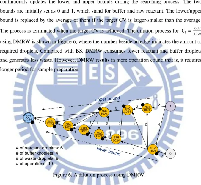
The algorithm for dilution and mixing with reduced wastage (DMRW) [27] is the first approach aiming at waste minimization by means of droplet sharing. The authors of DMRW claim that waste minimization is good for reducing reactant usage as well as droplet routing time. DMRW achieves target concentrations based on a binary search strategy. It continuously updates the lower and upper bounds during the searching process. The two bounds are initially set as 0 and 1, which stand for buffer and raw reactant. The lower/upper bound is replaced by the average of them if the target CV is larger/smaller than the average.
The process is terminated when the target CV is achieved. The dilution process for
using DMRW is shown in Figure 6, where the number beside an edge indicates the amount of required droplets. Compared with BS, DMRW consumes fewer reactant and buffer droplets and generates less waste. However, DMRW results in more operation count; that is, it requires longer period for sample preparation.
1024 607 # of reactant droplets: 6 # of buffer droplets: 4 # of waste droplets: 9 # of operations: 19 1 0 upper bound lower bound 1024 512 1024 768 1024 576 1024 640 1024 608 1024 592 1024 600 1024 604 1024 606 1 1 1 1 1 1 1 1 1 1 3 3 2 2 3 3 2 2 4 4
Figure 6. A dilution process using DMRW.
The improved dilution/mixing algorithm (IDMA) [28] is an improved version of DMRW.
For some target CVs, such as and , the dilution graph produced by DMRW is extremely unbalanced. In such cases, one of the two bounds varies frequently, and much waste droplets are thus produced. IDMA moderately relaxes the bound under certain conditions to make the dilution graph more balanced. For example, IDMA turns the dilution
graph in Figure 7(a) into the one in Figure 7(b) by relaxing the lower bound from to 0.
10
cases can be improved by IDMA. In most cases, IDMA even consumes more reactants, produces more waste droplets, and needs more operation counts than DMRW. Moreover,
IDMA may lead to imprecise target CV, such as
under Ct =
. It indicates that IDMA may induce a larger error than other approaches.
513 1024 # of reactant droplets: 6 # of buffer droplets: 5 # of waste droplets: 10 # of operations: 14 1 0 upper bound lower bound 1 1 514 1024 516 1024 520 1024 528 1024 544 1024 576 1024 640 1024 768 1024 512 1024 1 1 1 1 1 1 1 1 1 1 1 1 1 1 1 5 5 1
(a) An unbalanced dilution graph produced by DMRW.
513 1024 # of reactant droplets: 6 à 2 # of buffer droplets: 5 à 2 # of waste droplets: 10 à 3 # of operations: 14 à 10 1 0 upper bound lower bound 1 516 1024 528 1024 576 1024 768 1024 512 1024 1 384 1024 480 1024 504 1024 510 1024 1 1 1 1 1 1 1 1 1 1 1 1 1 1 1 1 1 1
(b) The dilution graph improved by IDMA Figure 7. A dilution process using IDMA.
3.1.3 REMIA
The reactant minimization algorithm (REMIA) [31] is the first algorithm which focuses on reactant minimization. For a given target CV, REMIA constructs a reactant-minimized mixing tree to guide the dilution process. Besides, REMIA utilizes essential reactant usage (ERU) of a mixing tree to estimate reactant usage, which gives a lower bound for reactant consumption. REMIA is a two-phased algorithm, including interpolated dilution phase and exponential dilution phase. In the interpolated dilution phase, REMIA decomposes the binary string of target CV in a top-down manner to construct the mixing tree with minimized ERU. In the exponential dilution phase, all leaf nodes of the mixing tree are generated through reactant-minimal exponential dilution process. This process guarantees minimal reactant usage. Figure 8 illustrates an example of REMIA for . The two phases are identified in Figure 8(a) and Figure 8(b) respectively.
# of waste droplets: 6 # of operations: 6 ERU: 1.8125 CV=0.10010111112 CV=12 CV=0.012 CV=0.000111112 CV=0.0012 CV=0.00011112 CV=0.0010111112 CV=0.0012 CV=0.0001112 CV=0.0012 CV=0.000112 CV=0.0012 CV=0.00012 PCV 607 1024 1024190 1024124 1024120 1024112 102496 102464 128 1024 128 1024 1024128 1024128 256 1024 1024 1024
(a) A mixing tree produced by REMIA.
PCV 256 1024 root(T1) root(T2) # of reactant droplets: 2 # of buffer droplets: 7 # of waste droplets: 2 # of operations: 7 128 1024 102464 128 1024 128 1024 128 1024 128 1024 256 1024 1024 1024 1024 1024 512 1024 256 1024 256 1024 512 1024
(b) The reactant-minimal exponential dilution process.
# of reactant droplets: 0 + 2 = 2 # of buffer droplets: 0 + 7 = 7 # of waste droplets: 6 + 2 = 8 # of operations: 6 + 7 = 13 ERU: 1.8125 (c) Total result.
12
REMIA can also be extended to deal with multi-target sample preparation problem. The extended version uses optimal unified exponential dilution process (OUED) to produce all leaf nodes required by the mixing trees for each Ct simultaneously, and further minimizes the
reactant usage. The details of mixing tree, ERU, reactant-minimal exponential dilution process, and optimal unified exponential dilution process (OUED) will be discussed in the following section.
3.2 Multi-Target Sample Preparation Algorithm
Intermediate droplet sharing algorithm (IDSA) [29] is the first algorithm to ensure concurrent preparation for multiple target CVs. The primary goal of IDSA is to minimize the number of waste droplets. More specifically, IDSA focuses on minimizing the number of intermediate CVs utilized in dilution process for waste and operation count reduction. In other words, the authors of IDSA believe that the number of waste droplets can be reduced through minimizing the number of intermediate CVs.
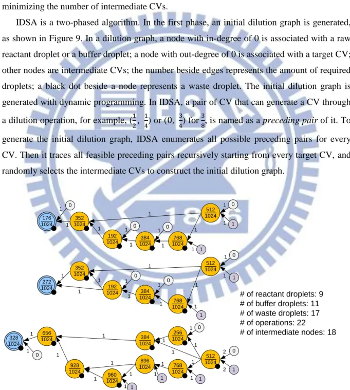
IDSA is a two-phased algorithm. In the first phase, an initial dilution graph is generated, as shown in Figure 9. In a dilution graph, a node with in-degree of 0 is associated with a raw reactant droplet or a buffer droplet; a node with out-degree of 0 is associated with a target CV; other nodes are intermediate CVs; the number beside edges represents the amount of required droplets; a black dot beside a node represents a waste droplet. The initial dilution graph is generated with dynamic programming. In IDSA, a pair of CV that can generate a CV through
a dilution operation, for example, ( ) or ( ) for , is named as a preceding pair of it. To generate the initial dilution graph, IDSA enumerates all possible preceding pairs for every CV. Then it traces all feasible preceding pairs recursively starting from every target CV, and randomly selects the intermediate CVs to construct the initial dilution graph.
272 1024 960 1024 328 1024 656 1024 512 1024 896 1024 928 1024 192 1024 768 1024 384 1024 384 1024 256 1024 512 1024 768 1024 0 0 0 1 0 0 1 1 1 0 1 1 1 1 1 1 1 1 1 1 1 1 1 1 1 1 1 1 2 2 176 1024 512 1024 768 1024 384 1024 0 0 0 0 1 1 1 1 1 1 1 1 1 1 1 1 1 1 352 1024 1 1 1 1 1 1 1 1 1 1 1 1 352 1024 192 1024 # of reactant droplets: 9 # of buffer droplets: 11 # of waste droplets: 17 # of operations: 22 # of intermediate nodes: 18
14
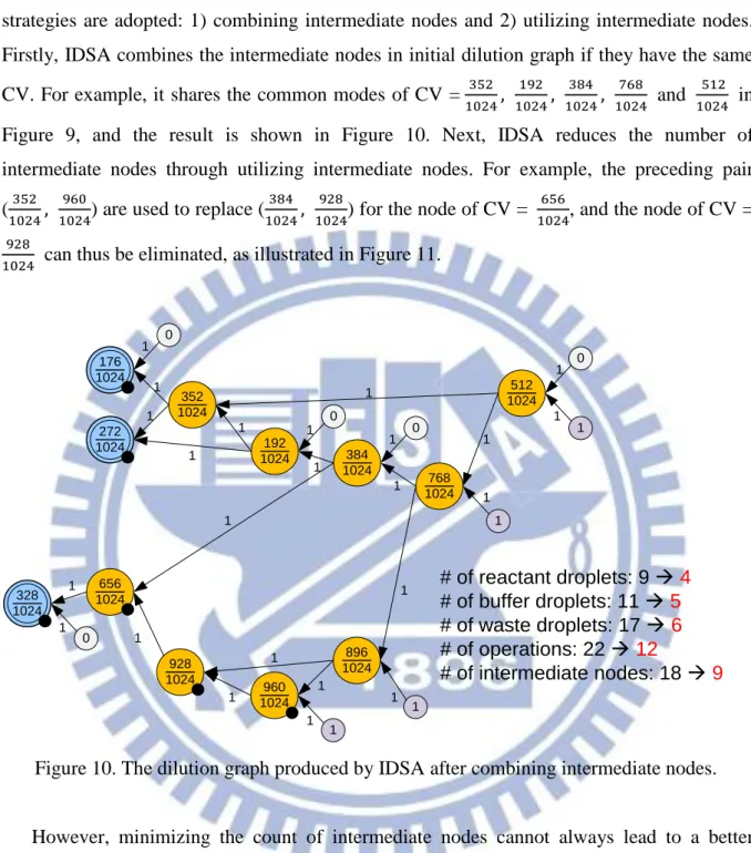
The second phase of IDSA tries to minimize the number of intermediate CVs. Two strategies are adopted: 1) combining intermediate nodes and 2) utilizing intermediate nodes. Firstly, IDSA combines the intermediate nodes in initial dilution graph if they have the same CV. For example, it shares the common modes of CV = and
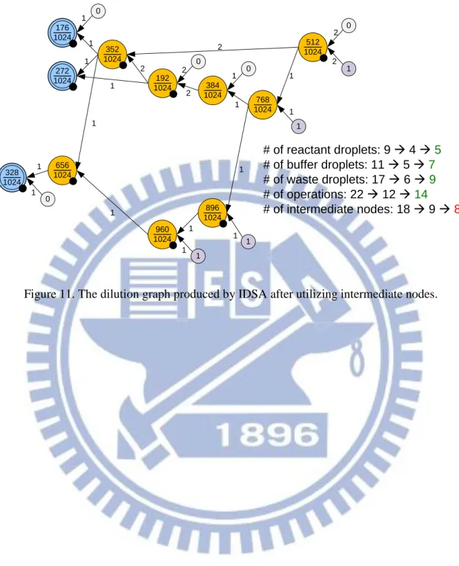
in Figure 9, and the result is shown in Figure 10. Next, IDSA reduces the number of intermediate nodes through utilizing intermediate nodes. For example, the preceding pair
( ) are used to replace ( ) for the node of CV = , and the node of CV =
can thus be eliminated, as illustrated in Figure 11.
272 1024 960 1024 176 1024 328 1024 656 1024 512 1024 896 1024 928 1024 192 1024 352 1024 768 1024 384 1024 0 0 0 0 1 1 0 1 1 1 1 1 1 1 1 1 1 1 1 1 1 1 1 1 1 1 1 1 1 1 1 1 1 # of reactant droplets: 9 à 4 # of buffer droplets: 11 à 5 # of waste droplets: 17 à 6 # of operations: 22 à 12 # of intermediate nodes: 18 à 9
Figure 10. The dilution graph produced by IDSA after combining intermediate nodes.
However, minimizing the count of intermediate nodes cannot always lead to a better result. This process may even increase the waste count, operation count and reactant usage. Figure 11 proves our concern that minimizing the number of intermediate nodes is not necessary reducing the waste amount. Therefore, a better indicator instead of intermediate CV count is required.
272 1024 960 1024 176 1024 328 1024 656 1024 768 1024 384 1024 0 0 0 0 1 1 0 1 1 2 2 2 2 1 1 1 1 1 1 1 1 1 1 1 1 1 2 2 1 1 1 896 1024 352 1024 192 1024 512 1024 # of reactant droplets: 9 à 4 à 5 # of buffer droplets: 11 à 5 à 7 # of waste droplets: 17 à 6 à 9 # of operations: 22 à 12 à 14 # of intermediate nodes: 18 à 9 à 8
16
Chapter 4 Problem Description
4.1 Mixing Tree
Unlike DMRW [27], IDMA [28], and IDSA [29] based on the dilution graph, another dilution strategy, mixing tree, is adopted by BS [26], RMA [29], and REMIA [31]. Here, we
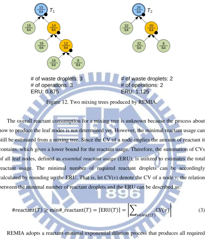
introduce mixing tree in detail. Two mixing trees produced by REMIA for and are shown in Figure 12. A mixing tree looks like a dilution graph, but there are some differences between them. A node with in-degree of 0 (i.e., leaf node) in a mixing tree is a PCV node instead of a reactant or a buffer droplet. A PCV node, defined by REMIA, is a node associated with PCV. Moreover, a mixing tree must be a full binary tree, that is, every branch node has exactly two children since a dilution operation requires two source droplets. However, only one of the two resultant droplets is utilized in the next dilution operations. As a result, a waste droplet must be produced at each branch node. The relation between the number of dilution operations, branch nodes, and waste droplets in a mixing tree T can be expressed as:
bran no e( ) operation( ) aste( ) (2) Note that there is a little difference between Equation (2) and the previous works like DMRW and IDMA, which define their equation as: operation( ) aste( ) . Previous works indicate that both two resultant droplets of target CV are useful and should not be considered as waste droplets. Nevertheless, we regard that only one of them s required; that is another one should be viewed as a waste droplet.
14 64 12 64 16 64 16 64 16 64 8 64 15 64 T1 20 64 32 64 32 64 26 64 T2 8 64 # of waste droplets: 3 # of operations: 3 ERU: 0.875 # of waste droplets: 2 # of operations: 2 ERU: 1.125
Figure 12. Two mixing trees produced by REMIA.
The overall reactant consumption for a mixing tree is unknown because the process about how to produce the leaf nodes is not determined yet. However, the minimal reactant usage can still be estimated from a mixing tree. Since the CV of a node implies the amount of reactant it contains, which gives a lower bound for the reactant usage. Therefore, the summation of CVs of all leaf nodes, defined as essential reactant usage (ERU), is utilized to estimates the total reactant usage. The minimal number of required reactant droplets can be accordingly calculated by rounding up the ERU. That is, let CV(v) denote the CV of a node v, the relation between the minimal number of reactant droplets and the ERU can be described as:
( ) ( ) ⌈ ( )⌉ ⌈∑ ( )
( ) ⌉ (3)
REMIA adopts a reactant-minimal exponential dilution process that produces all required leaf nodes of a mixing tree T with the minimal reactant usage. That is, ( ) ( ). This process is very similar to the well-known Huffman encoding algorithm [32]. Figure 13 illustrates this process for the mixing trees presented in Figure 12, where ( ) ⌈ ( )⌉ and ( ) ⌈ ( )⌉ .
18 64 64 32 64 16 64 32 64 16 64 16 64 16 64 8 64 PCVs of T1 # of reactant droplets: 1 # of buffer droplets: 4 # of waste droplets: 1 # of operations: 4 Reactant-minimal exponential dilution
(a) The reactant-minimal exponential dilution process for T1.
64 64 32 64 # of reactant droplets: 2 # of buffer droplets: 4 # of waste droplets: 3 # of operations: 4 64 64 32 64 16 64 8 64 PCVs of T2 32 64 Reactant-minimal exponential dilution
(b) The reactant-minimal exponential dilution process for T2. Figure 13. Reactant-minimal exponential dilution process for Figure 12.
Suppose there are more than one target concentration, REMIA can be extended by adopting an optimal unified exponential dilution (OUED) process to produce the leaf nodes of all mixing trees simultaneously. This process can further reduce reactant usage because:
⌈∑ ( )⌉ ∑⌈ ( )⌉ (4)
For example, the two individual reactant-minimal exponential dilution processes in Figure 13 is replaced by an optimal unified dilution process (OUED) shown in Figure 14, the number of required reactant droplets is thus reduced from 3 to 2. The amount of buffers, wastes, and operations are also reduced. Therefore, extended-REMIA provides a good initial solution for multi-target sample preparation. Moreover, it guarantees that the overall wasted reactant is less than one droplet because:
64 64 64 64 32 64 32 64 16 64 Optimal unified exponential dilution PCVs of T1 and T2 # of reactant droplets: 3 à 2 # of buffer droplets: 8 à 5 # of waste droplets: 4 à 0 # of operations: 8 à 5 32 64 16 64 16 64 16 64 8 64 8 64 32 64
20
4.2 Motivation
The major problem of a mixing-tree-based dilution process is excessive waste because every branch node always implies one waste droplet. The situation has become worse when multiple target CVs are considered. However, if one waste droplet produced in a mixing tree is useful for the other mixing tree while preparing multiple target CVs, it can be saved accordingly. For example, if the two mixing trees shown in Figure 15(a) share the same
branch node with CV =
, the overall ERU can be reduced from 2 to 1.375 and the number of waste droplets is decreased from 6 to 3, as depicted in Figure 15(b). The operation is named as droplet sharing, and it can effectively minimize both the reactant usage and the waste amount. # of waste droplets: 6 # of operations: 6 ERU: 2 12 64 15 64 23 64 16 64 8 64 16 64 32 64 14 64 16 64 16 64 16 64 8 64 12 64 14 64
(a) Two mixing trees for and .
# of waste droplets: 6 à 3 # of operations: 6 à 4 ERU: 2 à 1.375 8 64 16 64 32 64 12 64 14 64 16 64 16 64 15 64 23 64 (b) After sharing . Figure 15. A motivational example of droplet sharing.
In addition to droplet sharing, another strategy can also help to reduce the waste count. For example, Figure 16(a) illustrates the result after droplet sharing for three mixing trees for
and
. Among this graph, we find that the node with CV =
can be produced through recycling the waste droplets with CV = and respectively and applying an
interpolated dilution can thus replace the original one as shown in Figure 16(b). This recycling-then-replacing optimization strategy is called droplet replacement.
# of waste droplets: 6 # of operations: 7 ERU: 3.1875 22 64 12 64 27 64 18 64 32 64 32 64 16 64 8 64 4 64 32 64 15 64 14 64 16 64 16 64
(a) The result after droplet sharing
for and . # of waste droplets: 6 à 4 # of operations: 7 à 7 ERU: 3.1875 à 2.625 22 64 12 64 27 64 32 64 32 64 16 64 8 64 4 64 32 64 15 64 14 64 16 64 16 64 18 64
(b) The result after the branch node with
CV = is replaced.
Figure 16. A motivational example of droplet replacement.
The above two strategies show that both of them are useful for minimizing the reactant usage and the waste amount. More specifically, they turn the waste droplets into useful ones for reactant and waste minimization in multi-target sample preparation problem.
22
4.3 Problem Formulation
The multi-target sample preparation problem is formulated as follows. Given a set of target CVs, determine a dilution process under the (1:1) mixing model such that the reactant usage and the waste amount can be both minimized.
The proposed algorithm, WARA, which extensively exploits both droplet sharing and droplet replacement, is elaborated in the next chapter.
Chapter 5 Proposed Algorithm
In this chapter, we detail our multi-target sample preparation algorithm, waste recycling algorithm (WARA). Section 5.1 roughly describes the algorithm flow of WARA, which is composed of three consecutive phases. From Section 5.2 to section 5.4, we elaborate how the three phases work exactly.
5.1 Algorithm Overview
WARA divides a dilution process into three consecutive phases: Tree generation, droplet sharing, and droplet replacement. In the tree generation phase, WARA adopts the output of extended-REMIA [31] as its initial solution. In the second phase, WARA performs droplet sharing among all mixing trees for waste and reactant minimization. The dilution process is further refined via droplet replacement in the third phase. Finally, the optimal unified exponential dilution process (OUED) is followed to produce all required PCV nodes. The overall algorithm flow is illustrated in Figure 17.
Interpolated dilution Exponential dilution
OUED: optimal unified exponential dilution Phase 3: Droplet Replacement Phase 2: Droplet Sharing Phase 1: Tree Generation Target CVs OUED Final Result
24
5.2 Tree Generation
Tree generation is the first phase of WARA. In this phase, WARA generates a set of mixing trees with minimized ERU using REMIA [31] as initial dilution process. Each mixing tree is associated with a given target CV. According to the property of REMIA, all the
produced mixing trees are skewed. The two mixing trees for and are shown in
Figure 18. We adopt REMIA to produce initial mixing trees because REMIA is proven an effective method for reactant minimization in single-target sample preparation. Besides, other tree-based sample preparation methods like BS [26] can also be applied for tree generation in terms of different optimization goals, such as operation minimization. The comparison between experimental results obtained from different tree generation algorithms is shown in Chapter 6. # of waste droplets: 6 # of operations: 6 ERU: 2 12 64 15 64 23 64 16 64 8 64 16 64 32 64 14 64 16 64 16 64 16 64 8 64 12 64 14 64
5.3 Droplet Sharing
A branch node associated with a waste droplet is defined as a reusable node. For example, in Figure 18, the nodes with CV = and are all reusable nodes. In contrast, a branch node with no waste droplet is a reused node. For instance, the node with CV =
in Figure 19(a) is a reused node. The waste droplet of a reusable node can be utilized by another dilution operation through droplet sharing or droplet replacement. Note that each branch node is a reusable node in the initial mixing trees.
The first step of droplet sharing is identifying all sharable node pairs. A node pair (x, y) is sharable if both nodes are reusable nodes and CV(x) = CV(y). Assume (x, y) is a sharable node pair and node z represents the dilution operation which taking y as one of its source droplets, then z can take x as its source droplet instead of y since CV(x) = CV(y). As a consequence, x becomes a reused node since it is utilized at two different operations. At the same time, the subtree rooted at y can thus be safely eliminated. It is obvious that droplet sharing can effectively minimize both the reactant usage as well as the waste amount.
Suppose there exist more than one sharable node pairs at the same time, the order of pair selection does not affect the final result. That is, the outcome of droplet sharing is eventually identical no matter which node pair is selected first. For example, there are two sharable node
pairs in Figure 18, one is with CV = and the other is with CV = . Figure 19(a) shows the intermediate result as the node pair with CV = is selected for sharing first. Since there is
still one sharable node pair with CV = left in Figure 19(a), the succeeding operation can
thus be further performed. The final result is shown in Figure 19(b). On the other hand, if CV = is selected first, it still leads to the identical outcome in Figure 19(b). According to the example, it is clear that the order of pair selection has no effect on the outcome of droplet sharing.
26 reusable nodes reused node sharable node pair 8 64 16 64 16 64 16 64 32 64 16 64 14 64 14 64 12 64 15 64 23 64 # of waste droplets: 4 # of operations: 5 ERU: 1.625
(a) The intermediate result of droplet sharing.
# of waste droplets: 3 # of operations: 4 ERU: 1.375 8 64 16 64 32 64 12 64 14 64 16 64 16 64 15 64 23 64
(b) The final result of droplet sharing. Figure 19. Droplet sharing.
However, although the order of pair selection does not affect the final result, it does
impact the runtime efficiency. For example, if the node pair with CV = instead of is
selected first, only one sharing step is required to complete the droplet sharing process. It indicates that the farther a sharable node pair is from PCV nodes, the higher priority it should own because it can potentially eliminate the possible sharing for those sharable node pairs resided in larger fanin cone. This order decision strategy can improve the runtime efficiency and is exactly what Figure 18 and Figure 19 jointly demonstrate.
Furthermore, we find that for a node v, the number of nonzero bits in the binary representation of CV(v), denoted as nzb(v), can help us for deciding the sharing order. If x and y are two children nodes of node z, then the relation between their nzb number can be expressed as:
In other words, a node a must be farther from PCV nodes than the node b, if nzb(a) is larger than nzb(b). Therefore, in order to speed up the whole sharing procedure, the sharing must start from the pair with largest nzb to another with the smallest. The process of droplet sharing is not terminated until no sharable node pairs can be found. Figure 20 outlines the proposed droplet sharing flow.
DROPLET-SHARING(F)
// F is a forest containing a set of mixing trees
// every branch node in F is initially labeled as a reusable node
1. while (there is a sharable node pair)
2. identify a sharable node pair (x, y) with the largest nzb 3. for y’s fanout no e z, substitute y with x as z’s fanin no e 4. remove the subtree rooted at y
5. label x as a reused node
6. return the resultant dilution graph G
28
5.4 Droplet Replacement
In the end of droplet sharing phase, no sharable node pairs can be found anymore. However, some unpaired reusable nodes may still exist. Therefore, we further propose a method, which can keep recycling those remaining reusable nodes. Assume x and y are two reusable nodes and z is a node residing at neither x’s fanin cone nor y’s fanin cone; then the pair (x, y) is defined as a replacement candidate pair (RCP) of z if
( ) ( ) (7)
The resultant droplet of mixing the two waste droplets of x and y, denoted by w, can be utilized to replace z because CV(w) = CV(z). If this replacement happens, z and its exclusive fanin cone can thus be eliminated. Figure 21 illustrate the main concept of droplet replacement. It is clear that droplet replacement can also reduce the reactant usage as well as the waste amount simultaneously.
Figure 21. Droplet Replacement.
Unlike droplet sharing, the result of droplet replacement is order dependent. For example, for three reusable nodes x, y, and z, there may exist up to three feasible RCPs (x, y), (y, z), and (x, z). Nevertheless, no matter which RCP is selected for droplet replacement, it would make other two RCPs no longer feasible. For example, selecting (x, y) would make (y, z) and (x, z) no longer feasible because x and y become reused nodes, as illustrated in Figure 22.
(x, y)
(y, z)
(x, z)
RCPs
or
or
(x, y)
(y, z)
(x, z)
RCPs
(x, y)
(y, z)
(x, z)
RCPs
(x, y)
(y, z)
(x, z)
RCPs
Figure 22. Droplet replacement is order dependent.
Since the reactant minimization is the primary optimization objective of WARA, the strategy for RCP ordering should be a good idea to sort RCPs by total ERU saving. That is, an RCP with more ERU saving should be selected first for droplet replacement. Assume G/G’ are the graph before/after an RCP p is selected for droplet replacement, the gain of p is defined as:
( ) ( ) ( ) (8)
The droplet replacement process selects RCPs from the largest gain to the smallest one to achieve a maximal possible reactant reduction.
In the original definition, both two nodes within an RCP must be reusable nodes. However, feasible RCPs may be few if only the reusable nodes are considered, and the possibility of droplet replacement is thus limited. Consider the case illustrated in Figure 23(a), no feasible RCPs can be found for reactant minimization. However, if an additional PCV node is allowed while creating an RCP, it is likely that the overall ERU can be further minimized, just as Figure 23(b) shows. Therefore, the original definition of RCP is relaxed – for an RCP p, at most one of the two nodes can be a PCV node as long as gain(p) is positive. A loose upper bound on the number of maximum possible RCPs in a dilution graph G is , where k is the number of all branch and PCV nodes in G.
30 27 64 32 64 32 64 16 64 8 64 22 64 12 64 16 64 16 64 13 64 10 64 4 64 # of waste droplets: 5 # of operations: 5 ERU: 1.9375
(a) Two mixing trees for and .
27 64 32 64 32 64 16 64 8 64 22 64 12 64 13 64 4 64 # of waste droplets: 5 à 3 # of operations: 5 à 4 ERU: 1.9375 à 1.4375 RCP
(b) The result after droplet replacement.
Figure 23. An additional PCV node is allowed while creating an RCP.
If two or more RCPs are with the same largest gain, which is not uncommon, a tie-breaking score is required for a better result. As mentioned, if an RCP (x, y) is selected for droplet replacement, neither x nor y can appear in other RCPs later on since x and y are already reused. Suppose that RCP p = (x, y), RCP q = (x, z), RCP r = (z, w), and gain(p) = gain(q) > gain(r), the RCP p should have higher priority over the RCP q because 1) p is the only one chance for y to be reused and 2) z still has another chance (i.e., the RCP r) to be reused later even though the selection of p automatically invalidates q due to x, just as Figure 24 shows.
(x, y)
(x, z)
(z, w)
RCPs
p
r
q
or
(x, y)
(x, z)
(z, w)
RCPs
r
q
p
(x, y)
(x, z)
(z, w)
RCPs
r
q
p
Largest gain
Figure 24. The tie-breaking score (uniqueness) for droplet replacement.
To better formulate the above effect, we define the appearance count of node x, denoted as ac(x), as below
Obviously, the smaller the value of ac(x) is, the fewer chances (i.e., RCPs) x gets for being reused. Then, the uniqueness of RCP p(x, y), denoted as uniq(p), is accordingly defined as:
( ) { ( ) ( ) } (10)
As mentioned, the smaller the value of uniq(p) is, the higher priority p has. Hence, the uniqueness of RCP is used as the secondary key during RCP ordering. That is to say, an RCP is selected in decreasing order of gain(p) first, and then in the increasing order of uniq(p).
Figure 25 demonstrates an example of droplet replacement utilizing two different types of RCPs. Figure 25(a) gives an output right after droplet sharing. In the first iteration, the best RCP (i.e., the one with the highest precedence), which consists of two reusable nodes, is selected and the outcome is shown in Figure 25(b). In the next iteration, the new best RCP, which consists of a reusable node and a newly introduced PCV node, is chosen and the result is reported in Figure 25(c). The process of droplet replacement is not terminated until no RCP can be identified. Figure 26 outlines the proposed droplet replacement flow.
32 # of waste droplets: 8 # of operations: 8 ERU: 3.5625 27 64 32 64 32 64 16 64 8 64 22 64 12 64 16 64 16 64 13 64 10 64 4 64 20 64 32 64 32 64 32 64 8 64 26 64 29 64
(a) Initial graph G.
# of waste droplets: 8 à 6 # of operations: 8 à 8 ERU: 3.5625 à 2.9375 20 64 27 64 32 64 32 64 16 64 8 64 22 64 12 64 32 64 32 64 16 64 16 64 26 64 29 64 13 64 10 64 4 64 RCP
(b) After the first replacement.
# of waste droplets: 6 à 4 # of operations: 8 à 7 ERU: 2.9375 à 2.4375 27 64 22 64 32 64 32 64 16 64 8 64 13 64 4 64 12 64 20 64 32 64 32 64 26 64 29 64 RCP
(c) After the second replacement.
DROPLET-REPLACEMENT(G)
// G is a dilution graph right after droplet sharing
1. while (there is a replacement candidate pair (RCP) )
2. find all RCPs
3. calculate ac(v) for every node v in RCPs 4. calculate gain(p) and uniq(p) for every RCP p 5. sort all RCPs – primary: gain, secondary: uniq 6. identify RCP q(x, y) with the highest precedence
7. apply droplet replacement using q; update G accordingly 8. label x and y as reused nodes if not PCV nodes
return the resultant dilution graph G’
34
Chapter 6 Experimental Results
To further evaluate our algorithm, WARA, two sets of experiments are conducted in this chapter. In the former experiment, three consecutive phases within WARA are compared with each other. In the later, WARA is compared with a state-of-the-art multi-target sample preparation method. Furthermore, we discuss the effect of adopting different tree generation method in WARA.
6.1 Environment Setup
WARA has been implemented in C++/Linux environment. We compare WARA with an existing state-of-the-art method for multi-target preparation, IDSA [29]. In order to make the comparisons appropriate, the same experimental environment setup reported in IDSA is adopted. Various numbers of target CVs, ranging from 1 to 100, are considered, and every
target CV is randomly selected between and (i.e., precision level = 10). To make
the results more convincing, every reported value is an average of 1000 random cases in this paper instead of 20 in IDSA.
6.2 Results and Analyses
6.2.1 Three Consecutive Optimization Phases
Figure 27 illustrates the experimental flow and Table 1 shows the results after three consecutive optimization phases respectively. An optimal unified exponential dilution process (OUED) is followed by each phase. To evaluate our result, four counts for reactant (#R), buffer (#B), waste (#W), and operation (#OP), are reported.
Phase 1: Tree Generation Phase 2: Droplet Sharing Phase 3: Droplet Replacement Interpolated dilution Exponential dilution
OUED OUED OUED
Target CVs
OUED: optimal unified exponential dilution Result of Phase 1 Result of Phase 2 Final Result Waste Recycling Algorithm (WARA)
Figure 27. The experimental flow.
In Table 1, each row is associated with the results for a specified number of target CVs (#Ct). Note that the first row represents a special case, which is actually the result for
single-target sample preparation problem. In that case, WARA makes no improvement and performs the same with REMIA. However, it is absolutely correct because it can find neither a pair of branch nodes x and y in a skewed mixing tree with CV(x) = CV(y) nor a feasible RCP. Hence, it is undoubted that REMIA performs very well in single-target sample preparation. Besides, the remaining rows (i.e., multi-target cases) show a trend that the improvement due to droplet sharing and droplet replacement becomes more significant as #Ct
36
Table 1. Reactant/Buffer/Waste/Operation counts after the three optimization phases.
Tree Generation Droplet Sharing Droplet Replacement #Ct #R #B #W #OP #R #B #W #OP #R #B #W #OP
1 2.38 6.11 7.49 10.08 2.38 6.11 7.49 10.08 2.38 6.11 7.49 10.08 2 4.17 9.19 11.36 17.23 4.14 9.10 11.24 17.03 3.98 8.50 10.48 15.92 3 5.97 12.49 15.46 24.57 5.90 12.11 15.01 23.88 5.40 10.37 12.77 20.76 10 18.62 35.17 43.79 74.98 17.76 30.18 37.94 66.36 12.59 18.13 20.72 44.30 20 36.92 67.15 84.07 147.05 33.84 50.94 64.77 118.43 18.89 24.29 23.18 68.36 50 92.09 162.74 204.83 363.27 77.28 99.06 126.33 246.63 31.78 38.08 19.86 127.07 100 184.10 321.24 405.36 722.02 138.72 158.47 197.19 413.42 52.92 59.70 12.62 214.86
Figure 28 turns the data in Table 1 into Figures in terms of per-target basis. Reported data of tree generation are generally saturated at #Ct = 20, which indicates the saturation point of
the optimal unified exponential dilution process (OUED). However, both droplet sharing and droplet replacement constantly improve the outcome as #Ct gradually grows to 100.
Furthermore, the contribution of droplet replacement is more than droplet sharing in both reactant and waste minimization. Overall, WARA reduces #R/#W/#OP by 10%/17%/16% when #Ct is merely 3. As #Ct increases to 100, the reduction of reactant usage is 71%; the
reduction of operation count is 70%, which is notable since WARA does not pay extra attention on minimizing the operation count. More significantly, the waste amount is reduced by 97%, which concludes that WARA is very effective in waste minimization.
(a) Reactant count. (b) Buffer count.
(c) Waste count. (d) Operation count.
38
6.2.2 Sample Preparation with Different Tree Generation Techniques
Figure 29 presents the results among the three phases of WARA and IDSA in four different counts. Since IDSA only reports the waste and operation counts, reactant and buffer usage of IDSA is omitted in Figure 29. Note that the outcome of WARA’s first phase (i.e., tree generation) achieves almost the same quality as IDSA, which implies that the combination of the mixing trees and the optimal unified exponential dilution (OUED) technique (i.e., REMIA) is already a fairly good solution for multi-target preparation. Moreover, suppose we compare the outcome of WARA (i.e., the outcome after droplet replacement) with IDSA, WARA significantly outperforms IDSA as #Ct increase.
Specifically, WARA produces 48% less waste and requires 37% fewer operations than IDSA when #Ct = 10; the reduction further increases to 97% and 73% when #Ct grows to 100.
(a) Total reactant count. (b) Total buffer count.
(c) Total waste count. (d) Total operation count. Figure 29. Comparisons among the three phases of WARA and IDSA.
Figure 30 illustrates the results of three different multi-target sample preparation techniques, including WARA, WARA with BS (WARA-BS), and IDSA [29]. WARA-BS is a variant of WARA, which adopts mixing trees produced by BS [26] instead of REMIA in the first phase. BS is the approach which guarantees the minimal number of dilution operations for dealing with single-target sample preparation problem.
In Figure 30, we can find that WARA-BS consumes more reactant and buffer than WARA, which implies that adopting the mixing tree produced by REMIA as the initial dilution process is a better starting point than the one produced by BS in reactant minimization. On the contrary, WARA-BS requires fewer operations than WARA. The main reason is that the mixing trees produced by BS guarantee the minimal number of operations; it provides a better start point for operation minimization. Figure 30 also demonstrates that WARA-BS outperforms IDSA as well. We can conclude that the contribution jointly from droplet sharing and droplet replacement, which are the essential parts of WRA, is much more significant than that from initial tree generation. Finally, the experimental results also suggest that WARA is very time-efficient. It can finish the case with #Ct = 100 in just few seconds.
40
(a) Total reactant count. (b) Total buffer count.
(c) Total waste count. (d) Total operation count. Figure 30. Comparisons among WARA, WARA-BS, and IDSA.
Chapter 7 Conclusion
Sample preparation is an essential process in biochemical reactions, and many techniques have been proposed to address this issue recently. However, only one of them, IDSA, focuses on the multi-target sample preparation problem. In this thesis, we propose a new algorithm, WARA, which concentrates on reactant and waste minimization in multi-target sample preparation. WARA first generates a set of mixing trees for all required target concentrations as an initial solution, and then recycles waste droplets through droplet sharing and droplet replacement. For the droplet sharing, WARA uses number of nonzero bits (nzb) in the binary representation of CVs to speed up sharing process. During the droplet replacement, the replacement candidate pair (RCP) is proposed to guarantee that the count of waste droplets decreases monotonously. Two factors, gain and uniqueness, are used to determine the replacement order for better reactant usage and waste count. The experimental results demonstrate that all the three phases of WARA have their own contributions during optimization. Furthermore, WARA outperforms the existing state-of-the-art algorithm IDSA in terms of waste amount and operation count. WARA reduces the waste and operation count by 48% and 37% respectively when the number of target concentrations is ten. The reduction is increased to 97% and 73% when the number of target concentrations goes to hundred. Moreover, WARA is also very efficient in runtime. As a consequence, it is conclusive that WARA is currently the best method for multi-target sample preparation on digital microfluidic biochips.
42
References
[1] . Da an J. Finkelstein, “Insig t: Lab on a ip,” Nature, vol. 442, no. 7101, pp. 367– 418, Jul. 2006.
[2] A. Arora, G. Simone, G. B. Salieb-Beugelaar, J. T. Kim, an A. Manz, “Latest evelopments in mi ro total analysis systems,” Analyti al emistry., vol. 82, no. 12, pp. 4830–4847, 2010.
[3] R. B. Fair, A. Khlystov, T. D. Tailor, V. Ivanov, R. D. Evans, P. B. Griffin, V. Srinivasan, V. K. Pamula, M. G. Polla k, an J. Z ou, “ emi al an biologi al appli ations of digital-mi roflui i evi es,” IEEE Design & Test of omputers, vol. 24, no. 1, pp. 10–24, Jan. 2007.
[4] M. G. olla k, . B. Fair, an A. D. S en erov, “Ele tro etting-based actuation of liquid droplets for mi roflui i appli ations,” Applie ysi s Letters, vol. 77, no. 11, pp. 1725– 1726, Sep. 2000.
[5] . aik, . K. amula, an . B. Fair, “ api roplet mixers for igital mi roflui i systems,” Lab on a ip, vol. 3, no. 4, pp. 253–259, Sep. 2003.
[6] . Srinivasan, . amula, an . Fair, “An integrate igital mi roflui i lab-on-a-chip for lini al iagnosti s on uman p ysiologi al flui s,” Lab on a ip, vol. 4, no. 4, pp. 310–315, May 2004.
[7] T.-Y. Ho, K. akrabarty, an . op, “Digital mi rofluidic biochips: recent research and emerging allenges,” in ro ee ing of IEEE/A M/IFI International onferen e on Hardware/Software Codesign and System Synthesis, 2011, pp. 335–343.
[8] T.-Y. Ho, J. Zeng, an K. akrabarty, “Digital mi roflui i bio ips: a vision for fun tional iversity an more t an Moore,” in ro ee ing of IEEE/A M International Conference on Computer-Aided Design, 2010, pp. 578–585.
[9] M. Alistar, E. Maftei, . op, an J. Ma sen, “Synt esis of bio emi al appli ations on digital microflui i bio ips it operation variability,” in ro ee ing of Symposium on Design, Test, Integration and Packaging of MEMS/MOEMS, 2010, pp. 350–357.
[10] L. Luo an S. Akella, “Optimal s e uling of bio emi al analyses on igital mi roflui i systems,” IEEE Transactions on Automation Science and Engineering, vol. 8, no. 1, pp. 216–227, Jan. 2011.
[11] P.-H. Yuh, C.-L. Yang, and Y.-W. ang, “ la ement of efe t-tolerant digital microfluidic biochips using the T-tree formulation,” A M Journal on Emerging Technologies in Computing Systems, vol. 3, no. 3, pp. 13:1–13:32, Nov. 2007.
[12] Z. Xiao an E. F. Y. Young, “ la ement an routing for ross-referencing digital mi roflui i bio ips,” IEEE Transa tions on omputer-Aided Design of Integrated Circuits and Systems, vol. 30, no. 7, pp. 1000–1010, Jul. 2011.
[13] M. o an D. Z. an, “A ig -performance droplet routing algorithm for digital mi roflui i bio ips,” IEEE Transa tions on omputer-Aided Design of Integrated Circuits and Systems, vol. 27, no. 10, pp. 1714–1724, Oct. 2008.
[14] Y. Z ao an K. akrabarty, “ o-optimization of droplet routing and pin assignment in isposable igital mi roflui i bio ips,” in ro ee ing of A M International Symposium on Physical Design, 2011, pp. 69–76.
[15] C.-Y. Lin and Y.-W. ang, “ ross-contamination aware design methodology for pin- onstraine igital mi roflui i bio ips,” IEEE Transa tions on omputer-Aided Design of Integrated Circuits and Systems, vol. 30, no. 6, pp. 817–828, Jun. 2011.
[16] T.-W. Huang, S.-Y. Yeh, and T.-Y. Ho, “A net ork-flow based pin-count aware routing algorithm for broadcast-a ressing EWOD ips,” IEEE Transa tions on Computer-Aided Design of Integrated Circuits and Systems, vol. 30, no. 12, pp. 1786– 1799, Dec. 2011.
[17] P. Roy, H. Rahaman, R. Bhattacharya, and P. Dasgupta, “A best pat sele tion base parallel router for DMFBs,” in ro ee ing of IEEE International Symposium on Electronic System Design, 2011, pp. 176–181.
[18] D. Mitra, S. Ghoshal, H. Rahaman, K. Chakrabarty, and B. B. B atta arya, “On resi ue removal in digital mi roflui i bio ips,” in ro ee ing of ACM Great Lakes Symposium on VLSI, 2011, pp. 391–394.
[19] K. akrabarty, “Design automation an test solutions for igital mi roflui i bio ips,” IEEE Transactions on Circuits and Systems I: Regular Papers, vol. 57, no. 1, pp. 4–17, Jan. 2010.
[20] S. Sa a, A. akraborti, an S. oy, “An effi ient single-fault detection technique for micro-flui i base bio ips,” in ro ee ing of IEEE International onferen e on Advances in Computer Engineering, 2010, pp. 10–14.
44
[21] G. M. Walker, N. Monteiro-Riviere, J. Rouse, and A. T. O'Neill, “A linear ilution mi roflui i evi e for ytotoxi ity assays,” Lab on a ip, vol. 7, no. 2, pp. 226–232, Oct. 2007.
[22] H. en, . Srinivasan, an . B. Fair, “Design an testing of an interpolating mixing architecture for electrowetting-based droplet-on- ip emi al ilution,” in ro ee ing of IEEE International Conference on Solid-State Sensors, Actuators and Microsystems (TRANSDUCERS), 2003, pp. 619–622.
[23] H. Moon, A. R. Wheeler, R. L. Garrell, J. A. Loo, and C. J. Kim, “An integrate igital microfluidic chip for multiplexed proteomic sample preparation and analysis by MALDI-MS,” Lab on a ip, vol. 6, no. 9, pp. 1213–1219, Jul. 2006.
[24] E. J. Griffit , S. Akella, an M. K. Gol berg, “ erforman e characterization of a reconfigurable planar-array igital mi roflui i system,” IEEE Transa tions on Computer-Aided Design of Integrated Circuits and Systems, vol. 25, no. 2, pp. 345–357, Feb. 2006.
[25] T. Xu, . K. amula, an K. akrabarty, “Automate , a urate, and inexpensive solution-preparation on a igital mi roflui i bio ip,” in ro ee ing of IEEE Biome i al Circuits and Systems Conference, 2008, pp. 301–304.
[26] W. T ies, J. . Urbanski, T. T orsen, an S. Amarasing e, “Abstra tion layers for scalable mi roflui i bio omputing,” Natural omputing, vol. 7, no. 2, pp. 255–275, May 2008.
[27] S. oy, B. B. B atta arya, an K. akrabarty, “Optimization of ilution an mixing of bio emi al samples using igital mi roflui i bio ips,” IEEE Transa tions on Computer-Aided Design of Integrated Circuits and Systems, vol. 29, no. 11, pp. 1696– 1708, Nov. 2010.
[28] S. oy, B. B. B atta arya, an K. akrabarty, “Waste-aware dilution and mixing of bio emi al samples it igital mi roflui i bio ips,” in ro ee ing of IEEE/ACM Design, Automation & Test in Europe Conference & Exhibition, 2011, pp. 1059–1064.
[29] Y.-L. Hsieh, T.-Y. Ho, an K. akrabarty, “On-chip biochemical sample preparation using igital mi roflui i s,” in ro ee ing of IEEE Biome i al ir uits an Systems Conference, 2011, pp. 297–300.