正交分頻多工系統下運用壓縮取樣技術執行通道估測

國

立

交

通

大

學

電信工程學系

碩

士

論

文

正交分頻多工系統下運用壓縮取樣技術

執行通道估測

Channel Estimation in OFDM Systems Using

Compressive Sampling Technique

研 究 生：闕瑞慶

指導教授：吳文榕 博士

正交分頻多工系統下運用壓縮取樣技術執行通道估測

Channel Estimation in OFDM Systems Using Compressive

Sampling Technique

研 究 生：闕瑞慶 Student: Ruey-Ching Chiueh

指導教授：吳文榕 博士 Advisor: Dr. Wen-Rong Wu

國 立 交 通 大 學

電 信 工 程 學 系

碩 士 論 文

A Thesis

Submitted to Department of Communication Engineering College of Electrical and Computer Engineering

National Chiao-Tung University in Partial Fulfillment of the Requirements

for the Degree of Master of Science

In

Communication Engineering July 2010

Hsinchu, Taiwan, Republic of China

i

正交分頻多工系統下運用壓縮取樣技術執行通道估測

學生：闕瑞慶 指導教授：吳文榕 教授

國立交通大學電信工程學系碩士班

摘要

摘要

摘要

摘要

在正交分頻多工(OFDM)系統中，通道估測(channel estimation)經常是藉由安插在 OFDM 符元(symbol)間的領航訊號(pilot)來完成。但是領航訊號的使用卻會影響到系統的 效能，越多的領航訊號被安插在 OFDM 符號間則能傳送的資料量就越少，系統的傳送 速率(transmission rate)便會下降；此外，在某些系統中領航訊號的數量是有所限制的， 因此如何利用少量的領航訊號來達到準確的通道估測便成了一個值得探討的問題。近年 來，有研究提出一項名為 Compressive Sampling (CS)的新技術，宣稱只需要運用少許的 取樣值便能還原原始的訊號，只要該訊號本身擁有稀疏(sparse)的特性即可。而在時域上 的通道響應其非零的位置通常不多，符合 CS 技術的要求，因此我們可以將此技術應用 在通道估測的問題上。在本篇論文中，我們提出使用一個 Subspace Pursuit (SP)方法，證 明其在通道估測方面比現存應用 CS 技術的眾多方法有更佳的效能表現，並透過回授 (feedback)的機制使此方法能在領航訊號密度很低的時候仍保有好的準確度，最後我們延 伸此估測法至時變通道。透過模擬結果，可以看出我們所提出的通道估測法在高速移動 的環境中依然擁有很好的效能。

ii

Channel Estimation in OFDM Systems Using Compressive Sampling

Technique

Student: Ruey-Ching Chiueh Advisor: Dr. Wen-Rong Wu

Department of Communication Engineering

National Chiao-Tung University

Abstract

In pilot-assisted OFDM systems, the channel estimation problem is usually solved by the using the pilot subcarriers inserted in OFDM symbols. However, more pilots used will lead to lower transmission rate, and the number of pilots is sometimes limited due to the systems. So we are facing a problem to accurately estimate the channel response while using a small number of pilots. Recently, a novel technique called compressive sampling (CS) has emerged, asserting to recover the sparse signals with a few measurements. Since the number of non-zero taps in time-domain channel response is small, we can then apply the CS methods to the channel estimation problem in OFDM systems. In this thesis, we propose using a subspace pursuit (SP) algorithm which is shown to be superior to the existing CS methods in channel estimation. The performance of proposed method is also shown to be good when pilot density is very low by adding a decision-feedback mechanism. Then, our problem is extended to the time-variant case. And simulation results show the proposed method performs well even when the speed of mobility is high.

iii

誌謝

誌謝

誌謝

誌謝

本篇論文得以順利完成，首先必須要感謝我的指導教授 吳文榕老師，不論在學業 或研究問題上，老師總是扮演著明燈的角色，在我遭遇困境時適時的提供專業的意見與 指導，對於日常生活與生涯規劃，老師也總是給予相當的關心與建議。這兩年來，在教 授身上獲得的不僅僅是更深一層的專業知識，更重要的是學習到從事研究的方法、態度 與精神。 此外，我要感謝實驗室的學長姐與同學們，在這期間帶給我許多研究上的幫助、生 活中的樂趣以及寶貴的人生經驗談，使我的碩士生活充實了起來。我也要感謝 97 的同 學們，尤其是室友們，從大學時期以來同甘共苦經歷的這些時光，都將成為我珍惜的記 憶，希望未來大家能夠繼續保持連絡。 最後，我要感謝我的家人以及朋友們，因為有你們的支持與陪伴，我才有力量能夠 順利的完成碩士學位，僅以此文獻給你們。

iv

Catalog

摘要 ... i Abstract ... ii 誌謝 ... iii Catalog ... iv List of Tables ... vi

List of Figures ... vii

Chapter 1 Introduction ... 1

Chapter 2 Introduction to OFDM System and Compressive Sampling ... 4

2.1 OFDM system ... 4

2.1.1 Continuous-time OFDM signal model ... 6

2.1.2 Discrete-time OFDM signal model ... 8

2.1.3 Complete OFDM system ... 11

2.2 Compressive sampling ... 11

2.2.1 CS recovery methods ... 13

2.2.2 Robustness of CS theory ... 14

Chapter 3 Channel Estimation ... 17

3.1 Conventional least squares method ... 17

3.2 Compressive sampling approach ... 21

3.2.1 Matching pursuit (MP) algorithm ... 21

3.2.2 Orthogonal Matching pursuit (OMP) algorithm ... 23

Chapter 4 Proposed Subspace Pursuit Algorithm in Channel Estimation ... 25

4.1 Channel estimation in linear time-invariant (LTI) system ... 25

v

4.1.2 Channel estimation with insufficient pilots ... 29

4.2 Channel estimation in time-variant system ... 34

4.2.1 Linear approximation method of time-variant channel ... 35

4.2.2 Time-domain LS estimator in time-variant channel ... 36

4.2.3 Proposed method in time-variant channel estimation... 43

Chapter 5 Simulation Results ... 46

5.1 Results of LTI channel estimation ... 47

5.1.1 Performance of different CS methods in channel estimation ... 47

5.1.2 Simulation results of SP estimator with tap numbers are known ... 48

5.1.3 Simulation results of SP estimator with tap numbers are unknown ... 50

5.1.4 Simulation results of SP estimator with insufficient pilots ... 51

5.2 Results of time-variant channel estimation ... 55

5.2.1 Results of proposed time-variant channel estimator with normalized Doppler frequency of 0.0244 ... 55

5.2.2 Results of proposed time-variant channel estimator with normalized Doppler frequency of 0.1016 ... 57

Chapter 6 Conclusions and Future Works ... 59

vi

List of Tables

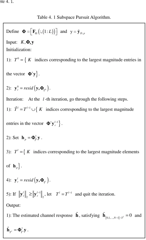
Table 3. 1: Matching pursuit algorithm ... 22 Table 3. 2: Orthogonal matching pursuit algorithm ... 24 Table 4. 1 Subspace Pursuit Algorithm. ... 26

vii

List of Figures

Figure 2- 1 Amplitude spectrum of an OFDM signal with N subcarriers. ... 5

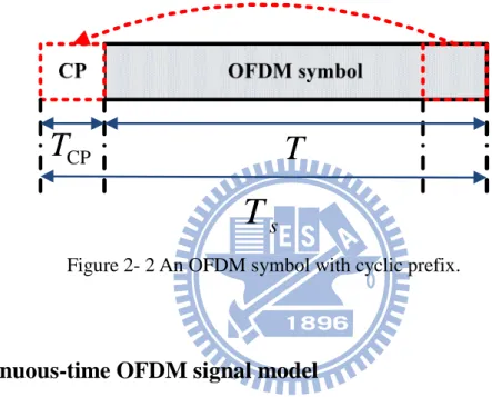
Figure 2- 2 An OFDM symbol with cyclic prefix. ... 6

Figure 2- 3 Continuous-time OFDM baseband modulator. ... 7

Figure 2- 4 Continuous-time OFDM baseband demodulator. ... 8

Figure 2- 5 Discrete-time OFDM system model. ... 9

Figure 2- 6 Block diagram of complete OFDM system. ... 11

Figure 3- 1 Example of subcarrier allocation in OFDM systems. ... 17

Figure 3- 2 Operations in MP algorithm... 22

Figure 3- 3 Operations in OMP algorithm. ... 23

Figure 4- 1 Operations in SP algorithm. ... 25

Figure 4- 2 Recursively conducted SP algorithm. ... 28

Figure 4- 3 Efficient recursively conducted SP algorithm. ... 29

Figure 4- 4 Aliasing in initial channel estimation... 30

Figure 4- 5 Initial channel estimation method. ... 31

Figure 4- 6 Data detection procedure. ... 32

Figure 4- 7 The proposed SP algorithm with insufficient pilot measurements. ... 33

Figure 4- 8 One time-variant tap. ... 34

Figure 4- 9 Linear approximation of a time-variant channel tap. ... 36

Figure 4- 10 The entries to be selected. ... 42

Figure 4- 11 Proposed method in time-variant channel. ... 44

Figure 5- 1 An example of a 6-tap channel. ... 47

Figure 5- 2 Performance comparison of different CS recovery methods. ... 48

Figure 5- 3 BER performance of proposed channel estimator for BPSK, QPSK, and 16-QAM with pilot density of 1/4. ... 49

viii

Figure 5- 4 BER performance of proposed channel estimator for BPSK, QPSK, and 16-QAM with pilot density of 1/8. ... 49 Figure 5- 5 Number of iterations required for SP re-conduction specified in Figure 4- 2 and Figure 4- 3. ... 50 Figure 5- 6 Performance of proposed channel estimator with pilot density 1/8 when tap

numbers are unknown. ... 51 Figure 5- 7 Performance comparison of different number of iterations for channel

re-estimation in BPSK. ... 52 Figure 5- 8 Performance comparison of different number of iterations for channel

re-estimation in QPSK. ... 53 Figure 5- 9 Performance comparison of different number of iterations for channel

re-estimation in 16-QAM. ... 53 Figure 5- 10 BER performance of proposed channel estimator with pilot density of 1/12 when tap numbers are known. ... 54 Figure 5- 11 BER performance of proposed channel estimator with pilot density of 1/12 when tap numbers are unknown. ... 54 Figure 5- 12 Performance comparison of proposed channel estimator with and without

re-estimation... 56 Figure 5- 13 Performance of proposed channel estimator with normalized Doppler frequency of 0.0244 for tap numbers are known. ... 56 Figure 5- 14 Performance of proposed channel estimator with normalized Doppler frequency of 0.0244 for tap numbers are unknown. ... 57 Figure 5- 15 Performance of proposed channel estimator with normalized Doppler frequency of 0.1016 for tap numbers are known. ... 58 Figure 5- 16 Performance of proposed channel estimator with normalized Doppler frequency of 0.1016 for tap numbers are unknown. ... 58

1

Chapter 1 Introduction

Wireless communication technique has attracted more and more attention in recent years since it can overcome the mobility problem. And the demand for high data rate transmission also emerges along with the popularity of high quality video and audio service. Orthogonal Frequency Division Multiplexing (OFDM) offers high spectrum efficiency and strong immunity to multipath fading channel and has become an important modulation technique in wideband wireless communications. It has also been widely used in many applications such as digital audio broadcasting (DAB), digital video broadcasting (DVB), wireless local area network (LAN), and WiMAX.

One of the most important tasks in OFDM receivers is to accurately estimate the channel response in order to recover the transmitted signals. To do that, a common practice is to insert pilot subcarriers in OFDM symbols. Since the data in pilot subcarriers are known, the related channel responses can be estimated and the response of other subcarriers can be interpolated [1],[2]. Pilot subcarriers cannot be used to transmit data and this approach affects the actual data rate. The more pilots we use, the lower the data rate will be. On the other hand, if the density of the pilot subcarriers is not high enough, the channel responses in data subcarriers cannot be accurately estimated and the data rate is affected also. In many applications, the time-domain channel response is sparse. In other words, the delay spread is large but the nonzero taps is a few. In these cases, a large number of pilots are still used. The sparsity of the channel is not explored.

In recent years, the compressive sampling (CS) technique has been developed to recover the sparse signals [3],[4]. Using the CS method, the number of measurements can be reduced dramatically since it exploits the sparse property of the signal. However, the complexity of the existing methods is high, despite the fact that some of them can be solved by the standard

2

linear programming (LP) [5]. Another way to reconstruct the sparse signal is using the greedy algorithm, which retrieves the desired signals from a large redundant set of vectors in an iterative fashion. The matching pursuit (MP) algorithm was developed and proved to be superior to the least squares (LS) algorithm [6],[7]. Later, the orthogonal matching pursuit (OMP) algorithm was introduced on purpose to overcome the re-selection problem occurred in the MP algorithm, and it also showed better performance than MP [8],[9]. Recently, a new method, called subspace pursuit (SP), was developed for the sparse signal reconstruction [10]. It has been shown that its computational complexity is lower than that of OMP and it can have the accuracy of LP.

The CS technique has found many applications in wireless communication, including the time-domain channel estimation in OFDM systems [11]. In the channel estimation of OFDM system, the received signals in pilot subcarriers serve as the measurements. As stated in [12],[13], sparse signals can be exactly recovered under the limited number of measurements when the sensing matrix satisfies the restricted isometry property (RIP). Thus, we can use a small number of pilots to recover the sparse channel response as long as RIP is held.

In this thesis, we study the spare channel estimation problem in OFDM systems. We first apply the SP algorithm and compare it with the LP, MP, and OMP algorithms. From simulation results, we show that SP indeed outperforms other methods. Next, we reduce the pilot density in order to raise the transmission rate. However, this causes aliasing in the time-domain channel response, and the response in the aliasing region cannot be recovered. To overcome the problem, we propose a decision-feedback method. The main idea is first to conduct an initial symbol detection with the partial aliasing-free channel response, and then use some decisions as pseudo pilots. With the original and pseudo pilots, the SP algorithm can then be conducted to estimate the whole channel response. Simulations results show that the proposed SP method works well even when the pilot density is low. Finally, we discuss the channel estimation problem in the high-mobility wireless environments, where the channel

3

becomes time-variant. In time-variant channel, the orthogonality of the subcarriers in one OFDM symbol is no longer held, causing the inter-carrier interference (ICI) effect. For ICI mitigation, accurate channel estimation is needed. We then extend the proposed decision-feedback SP algorithm to the channel estimation in time-variant channels. Simulations also show that the performance of the proposed method is satisfactory.

This thesis is organized as follows. First, we give an introduction to the OFDM system and show the main concepts and terminology of CS reconstruction technique in Chapter 2. In Chapter 3, various channel estimation methods are reviewed. In Chapter 4, decision-feedback SP algorithms for linear time-invariant and time-variant OFDM systems with uniformly distributed pilot subcarriers are proposed. In Chapter 5, we evaluate the performance of the proposed method and with simulations demonstrating its superior performance. Finally, the conclusions and future works are drawn in Chapter 6.

4

Chapter 2 Introduction to OFDM System and Compressive

Sampling

2.1 OFDM system

OFDM is a frequency division multiplexing (FDM) scheme and can be view as a digital multi-carrier modulation technique. In FDM, the high rate stream is divided into several parallel lower rate sub-streams, and this is equivalently to divide the available wideband channel into narrowband sub-channels, and each data stream is transmitted with a subcarrier in a sub-channel. While the data to be transmitted need not to be divided equally nor do they have to originate from the same information source.

The primary advantage of OFDM over single-carrier modulation is the resistance to the frequency selective fading effect. As the bandwidth of each OFDM sub-channel is sufficiently narrow, the effect of frequency selective fading for each transmitted signal in each sub-channel can be considered as flat. Thus, the equalizer at the receiver can be simplified to an one-tap frequency-domain equalizer. Furthermore, since the symbol duration increases for lower rate subcarriers, OFDM provides additional immunity to impulse noise and other impairments and the system stability is raised.

In OFDM systems, the subcarriers are designed to be orthogonal to each other, allowing the spectrum of individual subcarrier overlapping with minimum frequency spacing, achieving high spectral efficiency. Due to the orthogonality, the signal transmitted on each subcarrier can be recovered despite the overlapped spectrum. Figure 2- 1 shows the overlapped spectrum of OFDM modulated signals. Since the sinc-shaped spectrum of one subcarrier is required to be nulled at other subcarriers’ frequencies. The subcarrier spacing

5

between two neighbor subcarriers can be calculated as f W 1

N T

∆ = = , where W is the bandwidth, N is the number of subcarriers, and T is the symbol period.

W

f

N

∆ =

Figure 2- 1 Amplitude spectrum of an OFDM signal with N subcarriers.

In most wireless systems, signal usually travels through different paths causing the multipath effect, which results previous symbols to interfere with the latter symbols and the phenomenon is known as inter-symbol interference (ISI). By adding a cyclic prefix (CP) in front of each symbol, the OFDM scheme offers an effective solution for ISI mitigation. The size of CP is designed to be larger than the maximum channel delay spread, so that the effect of ISI is eliminated. Since CP is a copy of the end portion of an OFDM symbol, the transmitted signal becomes partially periodic, and the effect of the linear convolution with a multipath channel can be translated to a circular convolution. As is known, conducting a circular convolution in the time-domain is equal to conducting a multiplication in the frequency-domain. Thus, the received data in frequency-domain is simplified to a

6

point-to-point multiplication of the data symbol and channel frequency response. Moreover, if the CP length is long enough, the inter-carrier interference (ICI) can also be eliminated to maintain the orthogonality of subcarriers in the multipath fading environments. Figure 2- 2 shows the generation of the CP. In the figure, T denotes the symbol duration excluding CP,

CP

T the length of CP, and T the total symbol duration. _s

s

T

T

CP

T

Figure 2- 2 An OFDM symbol with cyclic prefix.

2.1.1 Continuous-time OFDM signal model

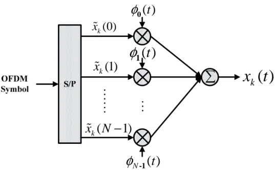
Figure 2- 3 shows a typical continuous-time OFDM baseband modulator. The operation of the modulation can be described as below. The transmitted symbol stream is first split into parallel sub-streams using a serial-to-parallel converter and each sub-stream modulates a subcarrier. The modulated signals are then transmitted simultaneously.

7

( )

t

φ

0

( )

t

φ

1

( )

N

t

φ

-1

∑

(0)

k

xɶ

(1)

k

xɶ

(

1)

k

x N

ɶ

−

( )

k

x t

Figure 2- 3 Continuous-time OFDM baseband modulator.

The i -th modulated subcarrier

φ

i( )t can be represented as

(t-CP) j2 k T CP 1 , [0, ) ( ) 0 , T s e t T T T t _T otherwise π φ  ∈ = +  =   i (2. 1)

In Figure 2- 3, x iɶk( ) denotes the transmitted symbol, drawn from a set of signal constellation

points, at the i-th subcarrier of the k -th OFDM symbol. The modulated baseband signal for the k -th OFDM symbol can then be expressed as

1 0 ( ) ( ) ( ) , ( 1) N k k i s s s i x t x i φ t kT kT t k T − = =

∑

ɶ − ≤ < + _{(2. 2)}

where N is the number of subcarriers. The received signal y t can be expressed as ( ) ( ) ( , ) ( ) ( )

y t =h t τ ∗x t +w t (2. 3)

where h t( , )τ _{denotes the time-variant channel impulse response at time t,} ( ) k( )

k

x t x t

∞ =−∞

=

∑

is the transmit signal, w t( ) _{is the additive white complex Gaussian noise, and} ∗ denotes the operation of linear convolution.

8

( )

y t

0

( )

t

ψ

1

( )

t

ψ

1

( )

N

t

ψ

−

(0)

k

yɶ

(1)

k

yɶ

(

1)

k

y N

ɶ

−

Figure 2- 4 Continuous-time OFDM baseband demodulator.

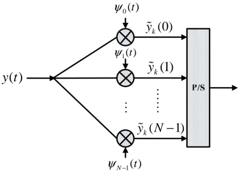
Figure 2- 4 shows a typical continuous-time OFDM baseband demodulator, in which ( )

i t

ψ denotes the matched filter for the i-thsubcarrier and y iɶ_k( ) _{is the demodulated signal} at i-th subcarrier for the k -th symbol. The matched filter is defined as:

( ) [0, ) ( ) 0 s i T t t T t otherwise φ ψ = ∗ − ∈  , , i (2. 4)

2.1.2 Discrete-time OFDM signal model

Consider an OFDM symbol, the modulated baseband signal is given by

2 1 0 1 ( ) 0 it N _j T i i x t x e t T T π − = =

∑

ɶ , ≤ ≤ _{(2. 5)}

where xɶ is the transmitted data symbol. Now, sampling the signal _i x t with the ( )

sampling period T_d T N

9

[ ]

( )

{ }

1 ₂ 0 2 1 N 0 1 1 , 0 1 N d d nT N _{j i} T i t nT i d j in N N i i i x n x t x e NT x e IDFT x n N π π − = = − = = = ∝ = ≤ ≤ −

∑

∑

ɶ ɶ ɶ (2. 6)

For a noise-freesystem, the discrete demodulated signal y kɶ

[ ]

_{can be expressed as:}

[ ]

1

[ ]

2

{ }

[ ]

N 0 1 = , 0 1 j kn N N n y k y n e DFT y n k N N π − − = =

∑

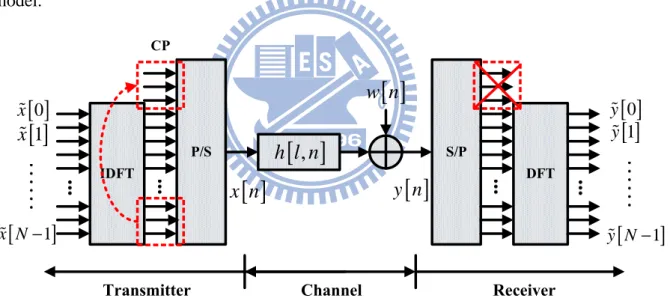
≤ ≤ − ɶ _{(2. 7)}

Equations (2. 6) and (2. 7)show that modulation and demodulation in OFDM systems can be conducted by inverse discrete Fourier transform (IDFT) and discrete Fourier transform (DFT), respectively. In practice, IDFT/DFT is implemented with inverse fast Fourier transform (IFFT)/fast Fourier Transform (FFT). Figure 2- 5 shows the discrete-time OFDM system model.

IDFT

P/S S/P

DFT CP

Transmitter Channel Receiver

[ ]

y n

[ ]

x n

[ ]

,

h l n

[ ]

w n

[ ]

0 yɶ

[ ]

1 yɶ

[

1

]

y Nɶ −

[ ]

0 xɶ

[ ]

1 xɶ

[

1

]

x Nɶ −

Figure 2- 5 Discrete-time OFDM system model.

Now, the modulation operation can then be summarized as follows. Data streams in the transmitter first modulate N subcarriers, which is performed by a N -point IDFT unit, and then a CP of length T is added in the time-domain symbol. The resultant signal _CP x n

[ ]

is then passed through a time-variant multipath channel. Assuming that both timing and carrier frequency synchronization are perfect, we can express the received signal y n

[ ]

at receiver as

10

[ ] [ ] [ ] [ ]

[ ]

(

(

)

)

[ ]

1 , , L N l y n h l n x n w n h l n x n l w n = = ⊗ +   =

∑

_ − _+ (2. 8)

where h l n

[ ]

, is the channel impulse response of the l -th tap at n-th time instant, L is the number of channel taps,

( )

⋅ _N represents a cyclic shift in the base of N , ⊗ is the circular convolution operator, and w n

[ ]

is sampled additive white Gaussian noise (AWGN) with variance σ2 .

Then a DFT is conducted for each symbol after CP removal, and the received signal in frequency-domain is given by

[ ]

[ ] [ ] [ ]

[ ] [ ] [ ]

1 0 , = , , 0 1 N m y k h k m x m w k h k k x k w k k N − = = + + ≤ ≤ −

∑

ɶ ɶ ɶ ɶ ɶ _{ɶ ɶ} (2. 9)

Equation (2. 9) can be expressed using a matrix equivalent model as

00 0 0 0 11 1 1 1 2 22 2 2 1 _{( 1)( 1)} 1 1 0 0 0 0 0 0 = 0 0 0 + 0 0 0 N _{N N} N N h y x w h y x w y h x w y _{− h} x ₋ w ₋ − −                                                           _ _    ɶ _⋯ ɶ ɶ ɶ ɶ ɶ ⋯ ɶ ɶ ɶ ɶ ⋯ ɶ ɶ ⋮ ⋮ ⋮ ⋮ ⋱ ⋮ ⋮ ⋮ ɶ _⋯ ɶ ɶ ɶ (2. 10)

where

[

x xɶ₀,ɶ₁,⋯,xɶ_N−1

]

T _{is the frequency-domain transmitted data vector,}

[

]

0, 1, , 1

T N

y yɶ ɶ ⋯ yɶ ₋

is the frequency-domain received data vector,

[

w wɶ₀, ɶ₁,⋯,wɶ_N−1

]

T _{is the AWGN noise vector,}

and diag

{

_hɶ₀₀,hɶ₁₁,⋯,hɶ_{(N−1)(N−1)}_

}

is an N N× matrix with _hɶ₀₀,hɶ₁₁,⋯,hɶ_{(N−1)(N−1)} _{as its}

11

2.1.3 Complete OFDM system

Channel coding / Interleaving Signal mapping (Modulation) S/P IFFT (OFDM modulation) Add CP P/S Channel DAC ADC S/P Decoding / Deinterleaving Signal demapping (Detection) P/S FFT (OFDM demodulation) Remove CP Input Data Source Output Data Source Channel Estimation Sybchronization AWGN

Figure 2- 6 Block diagram of complete OFDM system.

The block diagram of a complete OFDM system is shown in Figure 2- 6. The upper path denotes the transmitter chain, and the lower path is the receiver chain. At the transmitter, the data are first encoded by channel encoder, then interleaved and mapped onto QAM constellation. IFFT operation is then used as a modulator modulating each block of QAM symbols onto subcarriers. After that, a copy of the end portion of the symbol is added in front of each OFDM symbol as a CP. Finally, the baseband OFDM signal is passed to the digital-to-analog (D/A) converter, the RF circuit, and then transmitted. The receiver reverses the operations conducted at the transmitter. Note that synchronization and channel estimation have to be conducted firstly.

2.2 Compressive sampling

Conventionally, if we plan to reconstruct a sampled signal without any error, then a basic principle must be followed：The sampling rate must be at least twice the maximum frequency

12

contained within the signal. The principle is known as Nyquist/Shannon sampling theory, which is one of the crucial theorems in signal processing. However, a novel sampling theory called compressive sampling (CS) goes against this common principle has recently emerged [3],[4]. It asserts that if we know the signal itself is sparse (the support of the coefficient sequence is in a small set) or compressible (the sequence is concentrated near a small set) by some known transformation, then it is possible to uniquely recover the signal from far fewer measurements with high probability. The idea is that for a K-sparse signal, which there are only K coefficients supported on the signal, the unknowns of the signal are actually the K non-zero positions and K values.

Now, consider a general problem of recovering a signal ∈ N

x ℝ _{from a noiseless} measurement vector m k m  _∈  1 , 2 , ... , , ... ,  y = y y y y ℝ _where , , = 1,..., k = ϕk k m y x . (2. 11)

In other words, x is not directly observed. The measurements are obtained by correlating x with the waveforms N

k

ϕ ∈ℝ . In general, the system is “underdetermined” (m≪ N_{) in the} sense that the measurements are much less than the unknown signal values. Solving the ill-posed linear system of equations seems not possible. However, if signal x is sparse, which means the useful information content embedded in the signal is much smaller than its length/bandwidth, and the problem can be solved by the CS method, which exploits the sparsity and operates as we are directly capturing the information about the signal of importance.

13

2.2.1 CS recovery methods

Let ΦΦΦΦ be a matrix taking ϕ_k as its rows. The relation between the observation y and K-sparse signal vector x can be expressed as

0 ≤K y = x, xΦΦΦΦ (2. 12) where ∈ m N× ℝ Φ Φ Φ

Φ is referred to as the sensing matrix, and denotes the⋅ ₀ ℓ -norm. It has ₀ been shown that one can recover the signal x by solving an ℓ -norm minimization ₀ problem:

min x ₀ subject to y = xΦΦΦΦ (2. 13)

However, this approach cannot be used in practical since it is NP-hard [5],[14], and the computational complexity will be very high.

A more computationally efficient strategy was then proposed. The signal recovering problem is now reformulated as a convex optimization problem:

min x ₁ subject to y = xΦΦΦΦ (2. 14) where 1 1 N i i= =

∑

x x (2. 15)

denotes the ℓ -norm of ₁ x. This approach can be efficiently implemented by the standard process of linear programming (LP) [5],[15].

A Another way to estimate the sparse signals is the use of greedy algorithms such as Matching Pursuit (MP) [16],[17],[18], Orthogonal Matching Pursuit (OMP) [8],[9],[18], and Regularized Orthogonal Matching Pursuit (ROMP) [19], which iteratively decrease the approximation error by relaxing the sparsity constraint. These algorithms are operated as follows： Search for the supports of signal x by adding new candidates into the estimated

14

support set and subtract their contribution from the measurement vector y successively. The objective is to minimize the residue vector r_j =y - ΦΦΦΦ_jx_jat iteration j. The greedy algorithm provides an effective way to retrieve desired signals, referred as a small subset of vectors, from a large redundant set of vectors.

2.2.2 Robustness of CS theory

To study the reconstruction accuracy of CS, Restricted Isometry Principle (RIP) is introduced to describe the robustness of CS [5],[12],[20]. Let ΦΦΦΦ be a _T m×T matrix obtained by extracting the T columns of ∈ m N×

ℝ

Φ ΦΦ

Φ _with T 1 , ... , ⊂

{

N

}

. Then matrix ΦΦΦΦ

is said to satisfy the RIP if

(

)

2

(

)

2

1−δ_k x₂2 ≤ ΦΦΦΦ_Tx ≤ 1+δ_k x2₂ (2. 16) for all coefficient sequence x∈ℝT _{, T} ≤_{K, where K} ≤_{m is the sparsity of signal x,}

1

k

δ

≤ ≤

0 is the restricted isometry constant, and

1 2 2 2 1 N i i=   =  

∑



x x denotes the ℓ_2-norm.

The principle coveys that when the RIP is held, the columns of sensing matrix ΦΦΦ_{Φ are}

approximately orthogonal and the exact recovery achieves. A theorem has been proved in [5] that if signal x is K-sparse, and the restricted isometry constant satisfiesδ2k+δ3k < 1, the

solution of (2. 14) is exact. While the signal is just near sparse as a compressible signal, it has also been proved that the recovery error will be upper-bounded by

1 2 ˆ C K K − ≤ ⋅ x - x x x (2. 17)

for some positive constant C and restricted isometry constant δ_3k+δ_4k < 2, where ˆx is the solution of (2. 17), and x_Kis the best K-sparse approximations obtained by keeping K

15

largest coefficients of x [13].

One may ask how to design a sensing matrix whose columns of size K are nearly orthogonal. For what value of K is this possible? We give some possible sensing matrices in the following：

1)Gaussian measurements: The entries of the sensing matrix is obtained by sampling independent and identically distributed (i.i.d) entries from the normal distribution with zero mean and variance 1/ m . In this case, if the sparsity K obeys, i.e.,

log( / )

m

K C

N m

≤ (2. 18)

where C is a constant related to the restricted isometry constant, then the probability of exact recovery can be expressed as 1−O e( −γN)for some γ >0 [20],[21].

2)Binary measurements: The entries of the m N× sensing matrix is obtained by sampling independently the symmetric Bernouli distribution P _ij

K ± 1 1 ( = ) = 2 Φ Φ Φ Φ . When (2. 18) is

held, the probability of exact recovery is also proved to be 1−O e( −γN)for some γ >0 [20].

3)Fourier measurements: The m N× sensing matrix ΦΦΦΦ is obtained by selecting m rows from a N N× Fourier matrix randomly and the columns of ΦΦΦΦ are renormalized to have unit norms. Now, the constraint to the sparsity K is

6 (log ) m K C N ≤ (2. 19) and is refined as 4 (log ) m K C N ≤ (2. 20)

to maintain an overwhelming probability of recovery [20],[22].

4)Incoherent measurements: The sensing matrix is obtained by selecting m rows from an N N× orthonormal matrix U randomly, and the columns are normalized to be

16

signal from the ΨΨΨΨ domain to the ΦΦΦΦ domain. Then the exact recovery occurs if

2 4 1 (log ) m K C N µ ≤ ⋅ ⋅ (2. 21)

where µ= N⋅max_{i j,} ϕ ,ψ_{i j} is the mutual coherence betweenΨΨΨΨand ΦΦΦΦ.

In the real-world applications, noise is always present. As a result, (2. 12) becomes

0 ≤K

y = x + z, xΦΦΦΦ (2. 22)

where z is the noise vector with a bounded energy z 2₂ ≤σ2. The problem we have now is to solve the equation shown below:

2

min x ₁ subject to y - xΦΦΦΦ ≤σ _{(2. 23)}

From the CS theory, it asserts that the solution of (2. 23), ˆx_{, obeys}

2 2

2

ˆ− ≤ ⋅C Kσ

x x (2. 24)

for some constant C [13]. Therefore, the stability and robustness of CS are maintained. The CS technique has been widely applied in many areas. For example, it is used in data compression, sensor networks, and error correcting codes. Recently, it has been applied in channel estimation, which is what we are concerned in this thesis.

17

Chapter 3 Channel Estimation

In OFDM systems, there are mainly two types of subcarriers allocated, which is shown in Figure 3- 1. The data subcarriers as what it named are used to transmit data symbols, and the pilot subcarriers are the subcarriers, spread uniformly in the frequency-domain, used to conduct channel estimation.

Figure 3- 1 Example of subcarrier allocation in OFDM systems.

3.1 Conventional least squares method

Typically, channel estimation can be performed either in the time-domain or the frequency-domain. The time-domain received signal (after CP removal) can be expressed as

18

, 0

1

n n n n

y

= ⊗ +

h

x

w

≤ ≤ −

n

N

(3. 1) where N is the number of subcarriers, y is the time-domain received signal, _n x is the n

time-domain training symbols, h is the channel impulse response, and _n w is the AWGN n

noise. Reformulating (3. 1) in the matrix form, we can have

0 0 1 1 0 0 1 1 0 2 1 1 2 2 2 2 3 1 1 2 1 1 1 N N L N L N N N L N N N L N L N y x x x h w y x x x h w y h w x x x x x x y h w − − + − + − − − − − − − − − −                       ₌   ₊ _{= +}                 _ _          Xh w ⋯ ⋯ ⋱ ⋯ ⋮ ⋮ ⋮ ⋱ ⋮ ⋯ ⋯ ⋮ ⋮ ⋮ ⋯ ⋯ (3. 2)

where L is the maximum channel delay. A conventional method for channel estimation is the least-squares (LS) method. The LS channel estimate minimizes the squared errors given by：

2

ˆ

LS

y - Xh (3. 3)

where y =

[

y y₀, ₁,…,y_N−1

]

T _{is the time-domain received vector. The optimum estimate has} been solved as

(

)

1 ˆ H H LS − = h X X X y (3. 4)

The time-domain LS method described above requires a time-domain training sequence. Another LS channel estimation method, described below, uses pilot subcarriers. Consider a received OFDM symbol in the i-th subcarrier:

i i i i

y

ɶ

=

h x

ɶ

ɶ

+

w

ɶ

(3. 5)

where yɶ is the received signal in the frequency-domain, _i xɶ is the transmitted signal in the i

frequency-domain, hɶ is the channel frequency response, and _i wɶ is the corresponding AWGN _i noise. Note that hɶ can be expressed as _i hɶ _i = ⋅f h, where is h the channel response in the

19

time-domain expressed as a vector, and f is a row of the DFT matrix. Equation (3. 5) then becomes

i i i

y

ɶ

=

x

ɶ

fh

+

w

ɶ

(3. 6)

Considering the received signals in all pilot subcarriers, we can have following expression:

0 0 0 1 1 1 0 1 2 2 2 2 1 1 0 1 ( 1) 2 2 2 0 1 ( 1) 2 2 2 0 1 ( 1) 2 2 2 0 2 2 M M M p p p L j j j N N N p p p L j j j p _{N N N} p p p p L j j j N N N p p p p p j j N e e e y e e e y y _{e e e} y e e π π π π π π π π π π π − − − ∗ ∗ ∗ − − − − ∗ ∗ ∗ − − − − ∗ ∗ ∗ − − − − ∗ − −        ₌           X ⋯ ɶ ⋯ ɶ ɶ ɶ _⋯ ⋮ ⋮ ⋮ ⋱ ⋮ ɶ 0 1 2 1 1 1 0 1 2 1 1 ( 1) 2 M M p p p L _p p L j N N p p w h w h h w h w e π − − − ∗ ₋ ∗ −          _{  }    _{  }    _{  }    _{  +}    _{  }    _{  }    _{  }                 =X Fh + w ɶ ɶ ɶ ⋮ ⋮ ɶ ⋯ ɶ _ɶ (3. 7) where 0 1 2 1 0 0 0 0 0 0 0 0 0 0 0 0 M p p p p p x x x x ₋         =         X ɶ ⋯ ɶ ⋯ ɶ _{ɶ ⋯} ⋮ ⋮ ⋮ ⋱ ⋮ ⋯ (3. 8)

is a diagonal matrix with pilot signals as its diagonal elements, pi , 0≤ ≤i M −1 is the index for pilot location and M is the total number of pilots,

0 1 1 = , , , M T p yp yp yp ₋  yɶ ɶ ɶ … ɶ _{is the}

received frequency-domain vector on pilot locations, F is a partial DFT matrix obtained by selecting M rows from a N-point DFT matrix according to pilot positions and retaining the first L columns, h=

[

h h₀, ,₁ …,h_L−1

]

T_{is the time-domain channel impulse response, and}

0, 1, , M1

T p wp wp wp ₋ 

w =ɶ ɶ ɶ … ɶ _{is the noise vector. Using the LS channel estimator, the following} squared error is minimized:

20

2

ˆ p p LS

y - X Fhɶ ɶ (3. 9)

And the resultant time-domain LS channel estimation can then be derived as

(

)

1 ˆ H H H H LS p p p p − = h F Xɶ X Fɶ F Xɶ yɶ _{(3. 10)}

The time-domain LS algorithm requires O L

( )

3 arithmetic operations, so the computational complexity is high when L is large. But if only L′ significant taps where L′ is much less than L are taken into account, the computational complexity of the LS method can be reduced. For example, if only two taps in h are considered, say h and ₀ hL−1 , then only the first and the last column of F are required to use. Then, we have

0 0 0 1 1 1 0 1 2 2 2 2 1 1 0 1 ( 1) 2 2 2 0 1 ( 1) 2 2 2 0 1 ( 1) 2 2 2 0 2 2 M M M p p p L j j j N N N p p p L j j j p _{N N N} p p p p L j j j N N N p p p p p j j N e e e y e e e y y _{e e e} y e e π π π π π π π π π π π − − − ∗ ∗ ∗ − − − − ∗ ∗ ∗ − − − − ∗ ∗ ∗ − − − − ∗ − −        ₌           X ⋯ ɶ ⋯ ɶ ɶ ɶ _⋯ ⋮ ⋮ ⋮ ⋱ ⋮ ɶ 0 1 2 1 1 1 0 1 2 1 1 ( 1) 2 M M p p p L p p L j N N w h w h h w h _w e π − − − ∗ ₋ ∗ −          _{  }    _{  }    _{  }    _{  +}    _{  }    _{  }    _{  }                 ɶ ɶ ɶ ⋮ ⋮ ɶ ⋯ 0 0 0 1 1 1 2 2 2 1 1 1 0 ( 1) 2 2 0 ( 1) 2 2 0 ( 1) ₀ 2 2 1 0 ( 1) 2 2 M M M p p L j j N N p p p L j j N N p p p L j j N N p p L p p p L j j N N e e y e e y h y _{e e} h y e e π π π π π π π π − − − ∗ ∗ − − − ∗ ∗ − − − ∗ ∗ − − − − ∗ ∗ − − −       _{ }   _{ }   _{  }   _{=  }     _{   }   _{ }   _{ }             X ɶ ɶ ɶ ɶ ⋮ ⋮ ⋮ ɶ 0 1 2 M-1 p p p p w w w w         +_{ }         ɶ ɶ ɶ ⋮ ɶ (3. 11)

21

2 2× matrix. As a result, the computational complexity is reduced.

3.2 Compressive sampling approach

For most wireless channels, the delay spread may be large, but the number of non-zero taps is generally small. That raises the subject in exploiting the sparsity of the time-domain channel response in the channel estimation problem. Since we are dealing with a sparse channel, the CS methods introduced in Chapter 2 are applicable. In the channel estimation of OFDM systems, the number of measurements indicates the number of inserted pilots. Now, we express the frequency-domain received signal vector on pilot positions as

, D p = Ω p yɶ F h + eɶ _{(3. 12)} where h = h_ T 0_{1 ( - )×N L} _T with 01 ( - ) 1 ( - ) N L N L ×

× ∈ℝ being a zero vector, FΩ is a matrix

collecting the rows of a N-point DFT matrix according to pilot indices Ω =

{

p p0, 1,…,pM−1

}

,

and yɶD p,

( )

i = yɶp_i /xɶpi , eɶp

( )

i = wɶpi / xɶpi , 0≤ ≤i M −1. Equation (3. 12) can be compared

with (2. 22), indicating that F_Ω is a sensing matrix. Thanks to the CS theory, we can estimate the time-domain channel impulse response with low pilot density.

3.2.1 Matching pursuit (MP) algorithm

MP algorithm was the first developed greedy algorithm applying in channel estimation, and it has been shown that MP is superior to the traditional LS method introduced in 3.1 either in the aspect of accuracy or the computational complexity [6],[7]. The block diagram of the MP algorithm is shown in Figure 3- 2.

22 1 l r ∗ − y Φ ΦΦ Φ

}

l

T

{

1 l l

T

=

T

−

∪

-1 , _{l l} l r

ϕ ϕ

k k y

Figure 3- 2 Operations in MP algorithm.

We also summarize the operation of the MP algorithm in Table 3. 1.

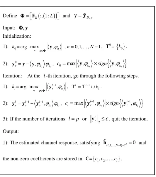
Table 3. 1: Matching pursuit algorithm

The MP algorithm first finds the column vector of ΦΦΦΦ having the maximum correlation with the measurement vector y. The column index is denoted by k₀ which is added into the

Define ΦΦΦΦ =_F_Ω

(

:, 1: L

( )

)

_ and y = yɶD p, Input: Φ,Φ,Φ,Φ,y Initialization: 1): ₀= arg max , _n , 0,1, , 1 n k n N ϕ∈ΦΦΦΦ y ϕ = … − ,

{ }

0 0 T = k . 2): 0 0 0 , r = − ϕ ϕk k y y y , c₀ =max y,ϕ_k0 ×sign

{

y,ϕ_k0

}

Iteration: At the l-th iteration, go through the following steps.

1): 1 = arg max l , l r n n k ϕ ϕ − ∈ΦΦΦΦ y , 1 Tl =Tl− ∪k_l. 2): 1 1, l l l l l r r r ϕ ϕk k − − = − y y y , c_l =max yl_r−1,ϕ_kl ×sign

{

yl_r−1,ϕ_kl

}

3): If the number of iterations l= p or

2

l r ≤ε

y , quit the iteration. Output:

1): The estimated channel response, satisfying hˆ_{{0,1, ,}…_{N− −1} T}l =0 and

23

index set T0. Then the k -th column of ₀ ΦΦΦΦ is selected to compute the residue vector y , 0_r

and the correlation coefficient. The process is then repeated, and the index set during each iteration is updated as 1 Tl Tl kl − = ∪ whenever 1 Tl l k ∉ − , otherwise Tl =Tl−1 . The algorithm is terminated when either the number of iteration exceeds a preset number, or the residue of the measurement vector is sufficiently small after l iterations.

3.2.2 Orthogonal Matching pursuit (OMP) algorithm

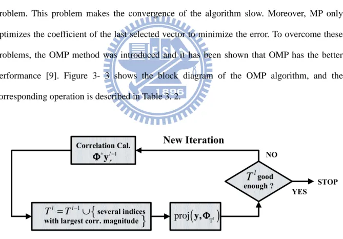
The MP algorithm searches all vectors in each iterative, leading to the re-selection problem. This problem makes the convergence of the algorithm slow. Moreover, MP only optimizes the coefficient of the last selected vector to minimize the error. To overcome these problems, the OMP method was introduced and it has been shown that OMP has the better performance [9]. Figure 3- 3 shows the block diagram of the OMP algorithm, and the corresponding operation is described in Table 3. 2.

Correlation Cal.

several indices with largest corr. magnitude

good enough ? 1 l r ∗ − y Φ ΦΦ Φ

}

New Iteration

YES NO STOP l

T

{

1 l l

T

=

T

−

∪

(

)

T proj y,ΦΦΦΦ l

24

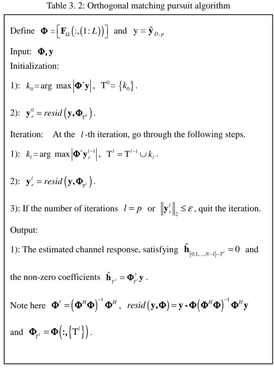
Table 3. 2: Orthogonal matching pursuit algorithm

The main difference between the MP and OMP algorithm is that the OMP maintains a stored dictionary containing all the indices selected among the iterations. The corresponding vectors are used to compute the new residue vector, avoiding the re-selection problem occurred in MP. The coefficients estimated in OMP are optimized with a set of selected vectors, which results in a much smaller error while the computational complexity is higher.

Define ΦΦΦΦ =_F_Ω

(

:, 1: L

( )

)

_ and y = yɶ_{D p,}

Input: Φ,Φ,Φ,Φ,y Initialization: 1): k₀= arg max ΦΦΦΦ∗y , T = k0

{ }

0 . 2):

(

0

)

0 T r =resid y y,ΦΦΦΦ .

Iteration: At the l-th iteration, go through the following steps. 1): k_l= arg max ΦΦΦΦ∗yl_r−1 , Tl =Tl−1∪k_l.

2):

(

_Tl

)

l

r =resid

y y,ΦΦΦΦ .

3): If the number of iterations l= p or

2

l r ≤ε

y , quit the iteration. Output:

1): The estimated channel response, satisfying _{{ }}

0,1, , 1

ˆ ₀

l

N− −T =

h … and

the non-zero coefficients _ˆ †

l l

T = T

h ΦΦΦΦ y.

Note here ΦΦΦΦ† =

(

Φ Φ ΦΦ Φ ΦΦ Φ ΦΦ Φ ΦH

)

−1 H, resid

(

y,ΦΦΦΦ

)

=y -Φ Φ Φ ΦΦ Φ Φ ΦΦ Φ Φ ΦΦ Φ Φ Φ

(

H

)

−1 Hy

and l

(

{ }

T

)

l T = Φ Φ :, Φ Φ :, Φ Φ :, Φ Φ :, .

25

Chapter 4 Proposed Subspace Pursuit Algorithm in Channel

Estimation

4.1 Channel estimation in linear time-invariant (LTI) system

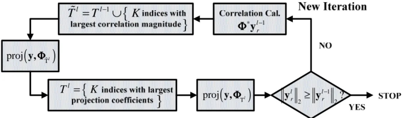
Recently, a new method, called subspace pursuit (SP), was developed for the CS signal reconstruction [10]. The computational complexity of the algorithm has been shown to be lower than that of OMP while the accuracy can approach that of LP. To the best of our knowledge, the SP method has not been used in the OFDM channel estimation problem. Here, we propose using the SP-based method in the channel estimation, and show that SP indeed outperforms the existing CS methods including LP, MP, and OMP by simulations. In this section, we only consider linear time-invariant (LTI) channels.

Recall that the received signal vector corresponding to the pilot sequence expressed as

,

D p

=

Ω p

y

ɶ

F h + eɶ

(4. 1)

with F is the sensing matrix, _Ω h the channel response, and eɶ_p noise. Let y = yɶ_{D p,} , a schematic diagram of the SP algorithm is shown in Figure 4- 1.

(

T

)

proj y,ΦΦΦΦl

(

T

)

proj y,ΦΦΦΦɶl 1 l r ∗_y − Φ Φ Φ Φ 1 2 2? l l r r − ≥ y y

{

1 l l

T

ɶ

=

T

−

∪

K

}

{

l T = K

}

26

The main operation steps of the SP algorithm are summarized in Table 4. 1.

Table 4. 1 Subspace Pursuit Algorithm.

In the SP algorithm, K indices corresponding to the largest magnitude entries in ΦΦΦΦ∗y

Define ΦΦΦΦ =_F_Ω

(

:, 1: L

( )

)

_ and y = yɶ_{D p,}

Input: K,Φ,Φ,Φ,Φ,y

Initialization:

1): T0 =

{

K indices corresponding to the largest magnitude entries in

the vector ΦΦΦΦ∗y

}

. 2):

(

0

)

0 T r =resid y y,ΦΦΦΦ .

Iteration: At the l-th iteration, go through the following steps. 1): Tɶl =Tl−1∪

{

K indices corresponding to the largest magnitude entries in the vector ΦΦΦΦ∗yl_r−1

}

.

2): Set h_p =ΦΦΦΦ_T†ɶly.

3): Tl =

{

K indices corresponding to the largest magnitude elements of h_p

}

. 4):

(

_Tl

)

l r =resid y y,ΦΦΦΦ . 5): If 1 2 2 l l r r − ≥

y y , let Tl =Tl−1 and quit the iteration. Output:

1): The estimated channel response ˆh , satisfying _{{ }} 0,1, , 1 ˆ ₀ l N− −T = h _… and † ˆ l l T = T h ΦΦΦΦ y.

27

are first selected to form an index set T0. Here, K denotes the channel sparsity, and the residue is computed with respect to ΦΦΦΦ_T0 obtained by collecting the K columns from ΦΦΦΦ

according to the elements stored in 0

T . During the iteration, an 2K index set is formed by K indices that maximizing the correlation between the columns of the sensing matrix and the residue vector united with the K indices found at the previous iteration. Then the size of this set is shrunk to K again by choosing K indices from the largest magnitude elements of h_p, and this index set can be viewed as a refinement to the indices obtained previously.

The SP algorithm is stopped when the residue vector derived is larger or equal to the preceding one. After convergence, the tap positions of the channel are then found with the index set, and the coefficient on the taps can be calculated by the LS method.

Due to the refinement, the indices that are mistakenly included in the index set can be removed in the following iterations, and so as the reliable candidates, which can be retrieved at any stage of the recovery process. This is different to the MP-based algorithms which generates the list of candidates sequentially without backtracking. So, more accurate indices of the sparse channel gains can be expected.

4.1.1 SP algorithm without information of tap numbers

The number of channel taps may be unknown to the receiver. Therefore, a revised version of the SP algorithm is needed. A simple idea is to conduct the SP method iteratively with an increasing tap number, and put a threshold on the estimated channel impulse responses. Since the gains of the insignificant taps are usually small, we expect that the number of estimated channel taps after thresholding will be the same whenever the tap number exceeds the channel sparsity K . This can then be used as the stop criterion to the SP algorithm. The flowchart of the proposed algorithm is depicted in Figure 4- 2.

28 SP Algorithm Thresholding Increase Tap Number

(

K,

)

SP Φ,Φ,Φ,Φ,y 1 K= +K l l -1 h = h ? l

h

No Yes STOP ,K =2, =0l y

An initial frequency domain channel estimation without interpolation

Figure 4- 2 Recursively conducted SP algorithm.

However, the number of the iteration of the algorithm proposed above can be large since the tap number of a channel can be large. If the statistics of the number of the channel taps were known a prior with the help of some statistical properties, we can then use the expected tap number as the first input instead of two used above. Next, we search forward and backward depending on whether the actual taps are more than or less than the expected tap number. In this way, the iteration needed for SP re-conduction will be dramatically reduced when tap numbers are large. This can be seen from the simulation result in chapter 5. Figure 4- 3 shows the flowchart of the modified recursively conducted algorithm.

The upper part of Figure 4- 3 is used to decide whether the true taps are more than or less than the expected ones. The idea is to run the SP algorithm twice. If the estimated channel response after thresholding process has the same tap number, then we know the tap number of the true channel is less than that of the assumed number. Then, go to the right section. Otherwise, go left.

29

(K, )

SP Φ,Φ,Φ,Φ,y

,K =Expected Tap Number l, =0

y 1 K= +K 1 K= +K K= −K 1 l l -1 h = h ?

1?

l

≥

l

h

,K = −K 2 y (K, ) SP Φ,Φ,Φ,Φ,y (K, ) SP Φ,Φ,Φ,Φ,y ,K = K +1 y l l-1 h = h ? h = h ? _{l l -1}

Figure 4- 3 Efficient recursively conducted SP algorithm.

4.1.2 Channel estimation with insufficient pilots

Now, if the pilot density is low, the channel estimate conducted by the SP method may be inaccurate. As mentioned in chapter 3, the pilot subcarriers are inserted uniformly in the spectrum. Since the channel is estimated by the pilot subcarriers, which is equivalent to

30

conduct a sampling on the frequency-domain channel response. As a result, the channel response in time-domain can be seen as periodic. If the sampling rate is not high enough, an effect similar to aliasing will occur. The effect is depicted in Figure 4- 4.

Figure 4- 4 Aliasing in initial channel estimation.

Suppose that the sampling period or we say the pilot interval isK, then the period of the time-domain channel estimate will be N K , denoted as / D , where N is the number of 1

subcarriers. Let the maximum delay spread of the channel be D , it can be easily observed ₂ that the aliasing problem occurs when D₂≥D₁. And the response in the aliasing area cannot be recovered.

We propose a decision-feedback method to overcome this problem. In the first step, we conduct an initial time-domain channel estimate using the pilots and only take the response in the non-aliasing region. Using the estimated channel frequency response, we can use the SP algorithm to conduct a refined channel estimation and then symbol detection. Finally, using some detected symbols as additional pseudo pilots, we can conduct the SP method again to re-estimate the channel. We now describe the proposed method in detail. With the help of

31

pilot subcarriers, we first obtain a frequency-domain channel response, and then transform the response to the time-domain. Selecting the response in the non-aliasing region and transform them back to the frequency domain, we then obtain a new frequency-domain channel estimate obtained. Figure 4- 5 shows the procedure. Since the aliasing area is not large, and the power of channel taps inside is usually small, the incomplete channel response can be used to recover data with an acceptable error probability.

Figure 4- 5 Initial channel estimation method.

Let hˆɶ_i denote the initial frequency-domain channel estimate. We then use the channel

response to detect symbols at designated subcarriers. As known, the received signal in the frequency-domain at a subcarrier in subcarrier index i can be expressed as yi =h xi i+wi

ɶ

ɶ ɶ _{ɶ ,}

32

signal, wɶ is AWGN noise. With the use of the zero-forcing (ZF) equalizer, the estimated _i

symbol at the i-th subcarrier can be calculated by ˆ ˆ i i i y x h = ɶ ɶ

ɶ . Then the data is sent to the

decision device to recover the original transmitted symbol. Let the detected symbol be denoted as ˆxɶ . The flowchart of this procedure is shown in Figure 4- 6. d

yɶ

ˆxɶ

ˆ

d

x

ɶ

Figure 4- 6 Data detection procedure.

With detected data in hand, we can then choose some of them as additional pilots, increasing the pilot density. By choosing sufficient pseudo pilots, the period of the time-domain channel estimate D will be larger than the maximum delay spread of the ₁ channel D . Therefore, aliasing will not occur. As long as aliasing does not occur, we can ₂ recover the whole channel response. The operation of the re-estimation can be performed as that of the channel estimation described previously, with the increased pilots that combining the original pilots and the pseudo pilots. To obtain better performance, the re-estimation can

33

be conducted iteratively until a convergence is achieved. The complete flowchart of the proposed SP algorithm used with insufficient pilot measurements is shown in Figure 4- 7.

1 re re N =N + ? re set N <N

=0

re

N

Figure 4- 7 The proposed SP algorithm with insufficient pilot measurements.

The operations conducted in Figure 4- 7 are summarized as follows：

1) Use the pilot subcarriers to obtain an initial frequency-domain channel estimate without interpolation.