模擬退火於圖形偵測及震測圖形上之應用

國

立

交

通

大

學

多媒體工程研究所

碩

士

論

文

模擬退火於圖形偵測及震測圖形上之應用

Simulated Annealing for Pattern Detection and Seismic Applications

研 究 生：陳楷儒

指導教授：黃國源 教授

i

模擬退火於圖形偵測及震測圖形上之應用

學生: 陳楷儒

指導教授: 黃國源教授

國立交通大學多媒體工程研究所碩士班

摘要

ii

Simulated Annealing or Pattern Detection and Seismic Applications

Student: Kai-Ju Chen

Advisor: Dr. Kou-Yuan Huang

Institute of Multimedia Engineering

National Chiao Tung University

ABSTRACT

Keywords: simulated annealing, global optimization, neural network, Hough transform, seismic pattern.

Simulated annealing algorithm is adopted to detect the parameters of ellipses, hyperbolas and lines in images and applied to seismic pattern detection. We define the distance from a point to a hyperbolic pattern such that the detection becomes feasible. The proposed simulated annealing parameter detection system has the capability of searching a set of parameter vectors with global minimal error with respect to the input data. Based on the average of the minimum distance, we propose a method to determine the number of patterns automatically. Experiments on the detection of ellipses, hyperbolas, circles and lines in images are quite successful. The detection system is also applied to detect the line pattern of direct wave and the hyperbolic pattern of reflection wave in the simulated and real one-shot seismogram. The results can improve seismic interpretations and further seismic data processing.

iii

誌

謝

感謝我的指導老師，黃國源教授。老師的辛勤指導與勉勵，使我得以順利完 成此論文。同時感謝參與口試的口試委員，劉長遠教授、蘇豐文教授以及王榮華 教授，由於您們的指導與建議，讓這篇論文更加完整和充實。

感謝Colorado School of Mine發展的Seismic Unix軟體與國科會的支持，讓本 計畫NSC 95-2221-E-009-221得以順利完成。

感謝我的家人，謝謝你們在全心全意地支持，讓我在這研究的路上走得更順 利，進而能無後顧之憂的學習，追求理想。感謝我的同學與朋友，在生活與學業 上互相勉勵，共同成長。

iv

Contents

Chapter 2 Simulated Annealing ... 3 

Chapter 3 Proposed System ... 6 

3.1  Definition of the system error ... 6 

3.1.1  Equation of the parametric pattern ... 6 

3.1.2  Distance from a point to a pattern ... 9 

3.1.3  Distance from a point to K patterns ... 11 

3.1.4  Error from N input data to K patterns in the system ... 12 

3.2  Simulated annealing parameter detection system ... 13 

3.2.1   Simulated annealing algorithm for parameter detection ... 13 

3.2.2   Simulated annealing algorithm to detect North‐South opening hyperbolas ... 15 

Chapter 4 Implementation and Experimental Results ... 20 

4.1  Detection of ellipses, hyperbolas, and lines ... 20 

4.2  Detection of North-South Opening Hyperbolas ... 31 

4.3  Determination of the Number of Patterns ... 34 

4.4  Seismic Applications on Simulated data ... 37 

4.5  Seismic Applications on Real Seismic Data ... 46 

Chapter 5 Conclusions and Discussions ... 59 

5.1  Conclusions ... 59 

5.2  Discussions ... 59 

v

List of Figures

Fig. 1. Illustration of descent and ascent direction. Dash arrow: ascent direction. Solid

arrow: descent direction. ... 4 

Fig. 2. Flowchart of the simulated annealing algorithm. ... 5 

Fig. 3. The system overview. ... 6 

Fig. 4. Illustration of axis rotation: rotate the axis counterclockwise by θ. ... 8 

Fig. 5. Illustration of translation: translate the origin to (mx, my). ... 8 

Fig. 6. (a) Distance from points to the circle x2 _{+ y}2 _{= 1. (b) Distance from points to} the circle 0.25x2 _{+0.25 y}2 _{= 0.25 ... 10} 

Fig. 7. (a) Distance from points to the ellipse 0.5x2 _{+ 2y}2 _{= 1. (b) Distance from points} to the ellipse 0.125x2 _{+ 0.5y}2 _{= 0.25. ... 10} 

Fig. 8. (a) Distance from points to the hyperbola x2 _{– y}2 _{= 1. (b) Distance from points} to the hyperbola 0.25x2 _{– 0.25y}2 _{= 0.25. ... 11} 

Fig. 9. Distance from a point to all patterns. i is the index of the input point. k is the index of the pattern, and K is the number of patterns. ... 12 

Fig. 10. Total error of the system and procedure of simulated annealing. ... 12 

Fig. 11. A trial of the center (mx, my). (a): original parameter. (b): trial parameter. (c): preserved parameter. ... 17 

Fig. 12. A trial of shape parameters b and a. (a): original parameter. (b): trial parameter. (c): preserved parameter. ... 18 

Fig. 13. A trial of rotation angle θ. (a): original parameter. (b): trial parameter. (c): preserved parameter. ... 18 

Fig. 14. A trial of f. (a): original parameter. (b): trial parameter. (c): preserved parameter. ... 19 

Fig. 15. Detection of ellipses – (a): 2 ellipses with noise. (b): error plot of (a) with cooling cycles... 21 

Fig. 16. Detection of ellipses – (a): 1 ellipse and 1 circle with noise. (b): error plot of (a) with cooling cycles. ... 22 

Fig. 17. Detection of hyperbolas − (a): 2 hyperbolas with noise. (b): error plot of (a) with cooling cycles. ... 23 

Fig. 18. Detection of hyperbolas − (a): 2 hyperbolas with noise. (b): error plot of (a) with cooling cycles. ... 24 

Fig. 19. Detection of ellipses and hyperbolas − (a): 1 ellipse and 1 hyperbola with noise. (b): error plot of (a) with cooling cycles. ... 25 

Fig. 20. Detection of ellipses and hyperbolas − (a): 1 ellipse and 1 hyperbola with noise. (b): error plot of (a) with cooling cycles. ... 26 

vi

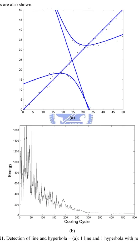
Fig. 21. Detection of line and hyperbola − (a): 1 line and 1 hyperbola with noise. (b): error plot of (a) with cooling cycles. ... 27  Fig. 22. Detection of lines by setting f = 0 − (a): 2 lines with noise. (b): error plot of (a)

with cooling cycles. ... 29  Fig. 23. Detection of lines by setting f = 0 − (a): 2 lines with noise. (b): error plot of (a)

with cooling cycles. ... 30  Fig. 24. Detection of hyperbolas − (a): 2 hyperbolas with noise. (b): Corresponding

plot of error vs. cooling cycles of (a). ... 32  Fig. 25. Detection of hyperbolas − (a): 2 hyperbolas with noise. (b): Corresponding

plot of error vs. cooling cycles of (a). ... 33  Fig. 26. Determination of number of patterns K. (a): K=1. (b): K=2. (c): K=3. (d): K=4.

(e): K=5. (f): Detection error of (a), (b), (c), (d) and (e). ... 35  Fig. 27. CPU time (in seconds) vs. number of patterns K. ... 36  Fig. 28. Illustration of horizontal reflection layer. ... 37  Fig. 29. Simulated seismic patterns − (a): Simulated one-shot seismogram (horizontal

reflection layer). (b): After envelope processing. ... 38  Fig. 30. (a): Result of thresholding from Fig. 29 with the threshold 0.15. The origin is

at the top-left corner. (b): Detected peak from (a). ... 39  Fig. 31. Detection of seismic patterns in Fig. 29 − (a): Detection result. (b): Error plot

with the cooling cycles... 40  Fig. 32. Illustration of dipping reflection layer. ... 41  Fig. 33. Simulated seismic patterns − (a): Simulated one-shot seismogram (dipping

reflection layer). (b): After envelope processing. ... 42  Fig. 34. (a): result of thresholding from Fig. 33(b) with the threshold 0.15. The

original is at the top-left corner. (b): detected peak from (a). ... 43  Fig. 35. Detection of seismic patterns in Fig. 33 − (a): Detection result. (b): Error plot

with the cooling cycles... 44  Fig. 36. Experiment on real data -- (a): Real seismic data from Canadian Artic. (b):

Plot of envelope. ... 48  Fig. 37. Experiment on real data -- (a): Threshold 0.15. (b): Detect peak. ... 49  Fig. 38. Experiment on real data -- (a): Choose peak with y < 700. (b): Detection

result of (a). ... 50  Fig. 39. Experiment on real data -- (a): Remove points nearest to the bottom pattern.

(b): Detection result. ... 51  Fig. 40. Plot detected curve on the original data -- (a): Detection result from Fig. 38

(b). (b): Detection result from Fig. 39 (b). ... 52  Fig. 41. Experiment on real data -- (a): Real seismic data from Gulf of Cadiz. (b): Plot of envelope. ... 54 

vii

Fig. 42. Experiment on real data – Thresholding result of the envelope in Fig. 41 (b) with threshold 0.5... 55  Fig. 43. Experiment on real data -- (a): Detected peak from Fig. 42. (b): Detection

result of (a), K = 2. ... 56  Fig. 44. Experiment on real data -- (a): Remove points nearest to the pattern around y

= 800 in Fig. 43 (b). (b): Detection result of (a), K = 1. ... 57  Fig. 45. Plot the detected curve in Fig. 44 (b) on the original data. ... 58  Fig. 46. Illustration of low initial temperature Tmax: (a) Detection result of Tmax=1. (b)

Accept ratio of larger-error parameters. ... 61  Fig. 47. Illustration of low initial temperature Tmax: (a) Detection result of Tmax=10. (b)

Accept ratio of larger-error parameters. ... 62  Fig. 48. Illustration of high initial temperature Tmax: (a) Detection result of Tmax =

100,000. (b) Accept ratio of larger-error parameters. ... 63  Fig. 49. Illustration of high initial temperature Tmax with more iterations: (a) Detection result of Tmax = 100,000. (b) Accept ratio of larger-error parameters. ... 64  Fig. 50. Enlarge the scale of points by 2: (a) Detection result of Tmax = 10. (b)

Detection result of Tmax = 100. ... 65 

Fig. 51. Relationship between Nt and detection result Tmax = 500: (a) Detection result

viii

List of Tables

Table I Relation between graph and parameters in (1) ... 7 

Table II Detection Error in Fig. 26 ... 34 

Table III CPU Time in Fig. 26 ... 34 

Table IV Detected parameters in Fig. 31 (a) in image space 512×65 ... 45 

Table V Detected parameters in Fig. 35(a) in image space 512×65 ... 45 

Table VI Detected parameters in Fig. 38 (b) with fixed f1 = 0 in image space 3100×48 ... 46 

Table VII Detected parameters in Fig. 39 (b) with fixed f1 = 0 in image space 3100×48 ... 47 

Table VIII Detected parameters in Fig. 43 (b) in image space 2050×48 ... 53 

1

Chapter 1

Introduction

Traditionally, the Hough transform (HT) is used to detect the parametric patterns such as lines and circles by mapping points in the image into the parameter space and

find the peak (maximum) in the parameter space[1]-[2]. The coordinate of the peak in

parameter space corresponds to a pattern in the image space.

Seismic pattern recognition plays an important role in oil exploration. In seismic data, a line represents the direct wave and a hyperbola represents the reflection wave [3]-[5]. In 1985, Huang et al. had applied the HT to detect line pattern of direct wave

and hyperbolic pattern of reflection wave in a one-shot seismogram [7]. However, it

was not easy to determine the peak in the parameter space and the large memory requirement was also a problem.

The Hough transform neural network (HTNN) was developed to solve the traditional HT problem [8]. It was designed to detect lines, circles, and ellipses by gradient descent to minimize the distance between points and patterns. HTNN was also adopted to detect lines and hyperbolas in a one-shot seismogram by Huang et al. [9]. The iterative method required less memory, but it had local minimum problem.

Simulated annealing (SA) was first proposed by Kirkpatrick in 1983 [10]. The algorithm simulates the procedure of the substance frozen from melt to a perfect crystal or low-energy state by careful annealing. The Metropolis criterion [11] which conditionally allows the state of the system to higher energy condition is the key of the SA algorithm to reach the global minimum. SA algorithm solves many combinatorial problems such as traveling salesman problem, circuit wiring problem,

and clustering problem [10], [12]-[16]. In 1987, Corana et al. applied the SA

algorithm to solve the global optimal solution of the continuous function [17] and compare it with simplex method [18] and adaptive random search [19]. The result shows the power of SA algorithm.

Here, we take the advantage of global optimization in SA to minimize the distance between points and patterns to detect parametric patterns: circles, ellipses, hyperbolas and lines. Also the proposed detection system is applied to the detection of line

2

pattern of direct wave and hyperbolic pattern of reflection wave in the simulated and real one-shot seismogram.

3

Chapter 2

Simulated Annealing

Optimization by SA is first proposed by Kirkpatrick et al. in 1983 to solve

combinatorial problem such as the placement and circuit wiring in chip design and

traveling salesmen problem [10]. The algorithm compares the optimization problem

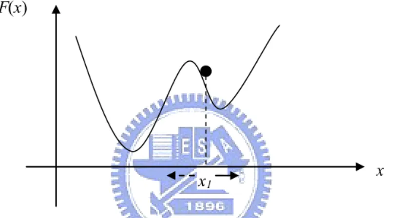
to cooling a fluid. A regular crystal has all atoms in the ground state or the lowest energy state by careful cooling procedure. In the procedure, the state of atoms is conditionally allowed to a higher energy state. Similarly, to achieve the optimal solution, the algorithm has to accept a solution with larger error in the procedure based on a criterion, Metropolis criterion [11]. Fig. 1 illustrates the function F(x) and the descent and ascent direction at x1. For the gradient descent algorithm, the direction for the next step is always descent. On the other hand, SA algorithm conditionally chooses ascent direction and this allows it to reach global minimum. The main steps of SA algorithm are in the following.

Algorithm: SA algorithm to get a configuration with lowest energy state. Input: A system with unknown minimum-energy configuration.

Output: A minimum-energy configuration.

Step 1: Initialization:

1. Set the initial temperature. 2. Set the initial configuration.

3. Define the temperature decreasing function. 4. Define the energy function.

Step 2: Give the configuration a random displacement then obtain a new configuration and a resulting energy change ∆E. To accept the displaced configuration or not is determined by Metropolis criterion. Metropolis criterion is a rule: If ∆E ≤ 0, the displaced configuration is accepted and treated as the starting configuration of the next step.

On the other hand, if ∆E ≥ 0, the acceptance of the displaced configuration is treated probabilistically:

1. Calculate prob = exp[-∆E/T(t)].

2. Generate a random number x. For convenience, random numbers uniformly distributed over (0, 1) are chosen.

4

3. If prob is greater than x, the new configuration is retained. Otherwise, the original configuration is used to the starting configuration of the next step. Repeat this step until equilibrium condition.

Step 3: When the equilibrium condition is reached, cool the system using the temperature decreasing function. Repeat this step until frozen condition.

In the SA algorithm, when to reach equilibrium condition and frozen condition is determined prior. For example, in step 2, the system reaches equilibrium condition in a specific temperature after 100 trials. Similarly, in step 3, frozen condition can be the temperature T < 0.001. Fig. 2 is the flowchart of the SA algorithm.

x1 x

F(x)

Fig. 1. Illustration of descent and ascent direction. Dash arrow: ascent direction. Solid arrow: descent direction.

5

YES

YES Start

Initialize: initial configuration, initial temperature, define energy function, temperature decreasing function

Randomly change configurations, and calculate ∆E

Accept new configurations ∆E≤0 Compute ) ) T( E exp( t prob= −Δ , Generate random number x

prob≥x Decrease the temperature Equilibrium condition? Frozen condition? Stop YES NO NO NO YES NO

6

Chapter 3

Proposed System

Fig. 3 is the overview of the proposed system. The detection system takes the N data as the input, followed by the SA parameter detection system to detect a set of parameter vectors of K patterns. After convergence, patterns are recovered from the detected parameter vectors.

Input

N data

Simulated annealing parameter detection system

Detected parameters

Detected

K patterns

Fig. 3. The system overview.

SA parameter detection system consists of two main parts: 1. definition of system error (energy, distance); 2. SA algorithm for determination of the parameter vectors with minimum error. To obtain the system error, we calculate the error or the distance from a point to patterns, and combine the errors from all points to patterns to be the system error.

3.1 Definition of the system error

To define the error or energy of the system, we first discuss the equation of the quadratic curve and the distance from a point to the pattern. Seconds, the error from a point to K patterns is the geometric mean of the distances from the point to all individual patterns. Finally, the system error is the arithmetic mean of the error of N points.

3.1.1 Equation of the parametric pattern

Circles, ellipses, and hyperbolas with rotations and translations can be expressed in the standard form in the translated and rotated coordinate system. That is, in translated and rotated coordinate system x″-y″, circles, ellipses, and hyperbolas can be expressed in the standard form as

f by

ax _''2+ _''2= _,

7

where a, b, and f control the graph of the equation. Table I lists the relation between the graph of the equation and parameters a, b, and f. If a > 0, b > 0, and f > 0 or a < 0,

b < 0, and f < 0, the graph is an ellipse; if a > 0, b < 0, and f ≠ 0 or a < 0, b > 0, and f ≠

0 the graph is a hyperbola. If a > 0, b < 0, and f = 0 or a < 0, b > 0, and f = 0, the graph represents the asymptotes of the hyperbola.

Table I

Relation between graph and parameters in (1)

a b f Graph ＋ ＋ ＋ Ellipse － － ＋ No graph ＋ － ＋ Hyperbola － ＋ ＋ Hyperbola ＋ － － Hyperbola － ＋ － Hyperbola ＋ ＋ － No graph － － － Ellipse ＋ － 0 Asymptote － ＋ 0 Asymptote ＋ ＋ 0 Point － － 0 Point

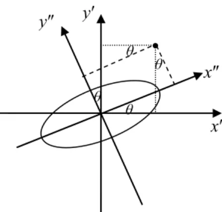
Since x″-y″ are the axes counter-clockwise rotated by θ from x′- y′, the relations of axes rotation are

θ θ 'sin cos ' '' x y x = + θ θ 'cos sin ' '' x y y =− + . (2)

Fig. 4 illustrates the relation. The equation of ellipses and hyperbolas after axes being rotated back to x′- y′ becomes

f y x b y x

8 θ x″ y″ y′ θ θ θ x′ 

Fig. 4. Illustration of axis rotation: rotate the axis counterclockwise by θ.

Since x′ and y′ axes translates the origin of x-y coordinate system to (mx, my), the

relations of translation are

y x m y y m x x − = − = ' ' . (4)

Fig. 5 illustrates the axes translation. And the equation in the x-y coordinate system is

f m y m x b m y m x

a_[( − _x)cosθ +₍ − _y)sinθ]2 + _[−₍ − _x)sinθ +₍ − _y)cosθ]2 = _.

(5) This can completely express any translated and rotated ellipse or hyperbola in 2D space.

So we can use (5) to represents any ellipse and hyperbola with the parameter, a, b,

f, θ, mx, and my. Parameter (mx, my)is the center; a, b, and θ are concerned about the

shape; f is related to the size. In the matrix form, a parameter vector, p = [mx, my, a, b,

θ, f]T represents a pattern. Since (5) represents the asymptotes or two crossing lines

when f = 0, we can use it to detect lines.

  (mx, my) x (0, 0) y y’ x’

9

3.1.2 Distance from a point to a pattern

Here, the detected patterns include ellipses, circles, hyperbolas, and lines. The distance from a point xi to the kth pattern is defined as

| ] cos ) ( sin ) ( [ ] sin ) ( cos ) [( | ) , ( 2 , , 2 , , k k y k i k x k i k k y k i k x k i k i i k f m y m x b m y m x a y x d − − + − − + − + − = θ θ θ θ (6)

Distance measure in (6) has a minimum d(xi, yi) = 0 when a = 0, b = 0, and f = 0.

However, these are not our desired parameters. Also, the distance from a point to the pattern is affected by the scale of coefficients. So we have to normalize the parameter

a and b.

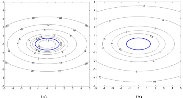
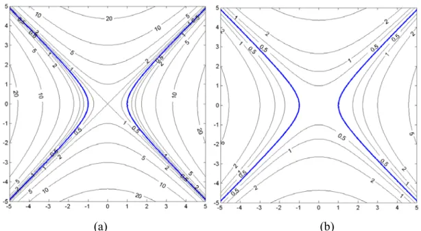
Fig. 6 (a) illustrates the distance from points to the circle, x2 _{+ y}2 _{= 1. Fig. 7 (a)} shows the distance from points to the ellipse, 0.5x2 _{+ 2y}2 _{= 1. Fig. 8 (a) illustrates the}

distance from points to the hyperbola x2 _{- y}2 _{= 1. Equal distance curves in those}

figures have corresponding distance 0.5, 1, 2, 5, 10, and 20. Fig. 6 (b) shows the

distance from points to the circle 0.25x2 _{+ 0.25y}2 _{= 0.25, which has the same shape}

with that in Fig. 6 (a), but all coefficients are 0.25 times smaller. The resulting distance in Fig. 6 (b) is shorter than that in Fig. 6 (a). Fig. 7 (b) and Fig. 8 (b) are illustrations of the distance but the coefficients are 0.25 times smaller than those in Fig. 7 (a) and Fig. 8 (b). This distance measure in (6) has a minimum distance, zero, when a, b, and f are all zeros. So we have to normalize parameters b and a. The

coefficients are normalized by | ab| so that |ab| = 1. This is similar to [8] where

the pattern is in the form xTAx = r2 and in order to reflect r in the distance, A is

normalized to ||det(A)|| = 1. Comparing this with (1), A = _⎥

⎦ ⎤ ⎢ ⎣ ⎡ b a 0 0 , ||det(A)|| = 1 implies |ab| = 1.

10

(a) (b)

Fig. 6. (a) Distance from points to the circle x2 + y2 = 1. (b) Distance from points to the circle 0.25x2 +0.25 y2 = 0.25

(a) (b)

Fig. 7. (a) Distance from points to the ellipse 0.5x2 + 2y2 = 1. (b) Distance from points to the ellipse 0.125x2 + 0.5y2 = 0.25.

11

  (a) (b)

Fig. 8. (a) Distance from points to the hyperbola x2 – y2 = 1. (b) Distance from points to the hyperbola 0.25x2 – 0.25y2 = 0.25.

3.1.3 Distance from a point to K patterns

Error or distance from a point to the patterns is defined as the geometric mean of the distances from the point to all patterns. The error of the ith point xi is

[

]

( _{i 1 i 2 i k i K i} K1

i E d d d d

E = x = x x x x (7)

where K is the total number of patterns. If the point is on any pattern, the error of this point will be zero. Fig. 9 shows the error of a point to all patterns. The distance layer computes the distance from a point to each pattern by (6), and the error layer outputs the error from a point to all patterns by (7).

12

Distance Layer: distance from a point to each pattern Error layer

Error from a point to all patterns xi yi Ei … … Ei= [d1(xi) d2(xi)… dk(xi)…dK(xi)]1/K Parameter vectors p = [mk,x, mk,y, ak, bk, θk, fk]T m1,x m1,y mk,x mk,y mK,x mK,y d1(xi) dk(xi) dK(xi)

dk(xi)=|a[(xi-mk,x)cosθk+(yi-mk,y)sinθk ]2

+b[-(xi-mk,x)sinθk+(yi-mk,y) cosθk]2-fk|

Fig. 9. Distance from a point to all patterns. i is the index of the input point. k is the index of the pattern, and K is the number of patterns.

3.1.4 Error from N input data to K patterns in the system

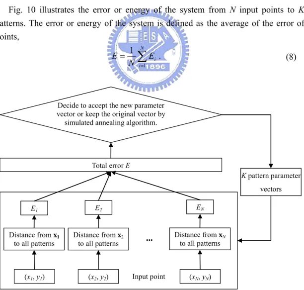
Fig. 10 illustrates the error or energy of the system from N input points to K patterns. The error or energy of the system is defined as the average of the error of points,

∑

Decide to accept the new parameter vector or keep the original vector by

simulated annealing algorithm.

... E1 (x1, y1) EN (xN, yN) Input point E2 Distance from x2 to all patterns (x2, y2) Distance from xN to all patterns Distance from x1 to all patterns K pattern parameter vectors

13

3.2 Simulated annealing parameter detection system

We use SA to detect the parameter vector of each pattern.Our goal is to find a set

of parameter vectors that can globally minimize the error of the system. Using the temperature decreasing function T(t)

T(t) = Tmax × 0.98(t-1) for t = 1, 2, 3, … (9)

as in[10].

Adjusting all parameters at one time is not efficient in convergence [8]. We use four steps in adjusting parameters also. The adjusting order is the center (mx, my), the

major and minor axes, b and a, and then the rotation angle θ, followed by the size r. The followings is algorithm to detect ellipses, hyperbolas, and lines. Here, lines are considered as the asymptotes of hyperbolas.

3.2.1 Simulated annealing algorithm for parameter detection

This algorithm is the general algorithm to detect ellipses, hyperbolas, and it treats lines as asymptotes of hyperbolas. Also, from Table I, the change of the signs of a, b, and f simultaneously makes the same patterns. So we have the constraint f ≥ 0 in the algorithm.

Algorithm: SA algorithm to detect parameter vectors of K patterns including ellipses,

circles, hyperbolas, and lines as asymptotes.

Input: N points in an image. Set K as the number of patterns. Output: A set of detected K parameter vectors.

Step 1: Initialization.

In the initial step t = 1, choose T(1) = Tmax at high temperature, and define the temperature decreasing function as in (9), T(t) = Tmax × 0.98(t-1)

Initialize parameter vectors p1, p2, ..., pk, …, pK, where pk = [mx,k, my,k, ak, bk, θk, fk]T, one p is for one pattern, and set P = (p1, p2, ..., pk, …, pK).

Calculate energy E(P) as (6), (7), and (8).

Step 2: Randomly change parameter vectors and decide the new parameter vectors in the same temperature.

For m = 1 to Nt (Nt trials in a temperature) For k = 1 to K (k is the index of the pattern)

14

Start a trial, including (a), (b), (c), and (d) in the following. (a) Randomly change the center of the kth pattern:

n m T y k x k T k,y x k m' m m m' ] =[ ] +α [ _{, , ,} , (10)

where n = [n1 n2]T is a 2 × 1 random vector, n1 and n2 are Gaussian random

variables with N(0, 1) and αm is a constant. Now, p’k = [m’k,x, m’k,y, ak, bk, θk, rk]T, and P’= (p1, p2, …, p’k,…, pK).

Calculate the new energy E(P’) from N points to K patterns. Using Metropolis criterion decides whether or not to accept P’: If the new energy is less than or equal to the original one, ∆E = E(P’) - E(P) ≤ 0, accept P’. Otherwise, the new energy is higher than the original one, ∆E = E(P’) - E(P) > 0. In this case, it computes prob = exp[-∆E/T(t)], and generates a random number x uniformly distributed over (0, 1). If prob ≥ x, accept P’; otherwise, reject it, and keep P. (b) Randomly change the shape parameters:

n ab k k k k b a b a' ' ]=[ ]+α [ , (11)

and normalize it by |a'_kb'_k|, where n = [n1 n2]T is a 2 × 1 random vector, n1

and n2 are Gaussian random variables with N(0, 1) and αab is a constant. Now,

p’k = [mk,x, mk,y, a’k, b’k, θk, rk]T, and P’ = (p1, p2, …, p’k,…, pK).

Similar to Step 2(a), calculate the new energy E(P’) from N points to K patterns. Using Metropolis criterion decides whether or not to accept P’. (c) Randomly change the angle:

n

k

k θ αθ

θ' = + , (12)

where n is a Gaussian random variable with N(0, 1) and αθ is a constant. Here,

the angle is in degree. Now, p’k = [mk,x, mk,y, ak, bk, θ’k, rk]T, and P’ = (p1,

p2, …, p’k,…, pK).

Similar to Step 2(a), calculate the new energy E(P’) from N points to K patterns. Using Metropolis criterion decides whether or not to accept P’. (d) Randomly change the size:

| |

' f n

f _k= _k +α_f , ₍₁₃₎

where n is a Gaussian random variable with N(0, 1) and αf is a constant. Now,

15

Similar to Step 2(a), calculate the new energy E(P’) from N points to K patterns. Using Metropolis criterion decides whether or not to accept P’. End for k

End for m

Step 3: Cool the System.

Decrease temperature T according to the cooling function (9), T(t) = Tmax ×

0.98(t-1), for t = 1, 2, 3, …, and repeat Step 2, and 3 until the temperature is low enough, for examples, repeat 500 times.

3.2.2 Simulated annealing algorithm to detect North-South opening hyperbolas

For seismic applications, patterns of reflection wave are North-South opening hyperbolas. Besides, patterns of direct waves are asymptotes of hyperbolas [3]-[5]. Equation of a North-South opening hyperbola is

f m y b m x a₍ − _x)2 + ₍ − _y)2 = _. (14) with a < 0, b > 0, f ≥ 0. So the parameters to be detected are p = [mx, my, a, b, f]T and

the distance from a point to a pattern becomes

| ) ( ) ( | ) , ( 2 , 2 ,x i ky k k i i i k x y a x m b y m f d = − + − − . (15)

We consider these properties and modify the algorithm to be just for North-South opening hyperbolas. This algorithm proves the detected patterns have the properties of North-South opening hyperbolas.

Algorithm: SA algorithm to detect parameter vectors of K North-South opening

hyperbolas.

Input: N points in an image. Set K as the number of patterns. Output: A set of detected K parameter vectors.

Step 1: Initialization.

In the initial step t = 1, choose T(1) = Tmax at a high temperature, and define

the temperature decreasing function as in (9), T(t) = Tmax × 0.98(t-1).

Initialize parameter vectors p1, p2, ..., pk, …, pK, where pk = [mk,x, mk,y, ak, bk, fk]T, one p is for one North-South opening hyperbola, and set P = (p1, p2, ...,

pk, …, pK).

16

Step 2: Randomly change parameter vectors and decide the new parameter vectors in the same temperature.

For m = 1 to Nt (Nt trials in a temperature) For k = 1 to K (k is the index of the pattern)

Start a trial, including (a), (b), and (c) in the following. (a) Randomly change the center of the kth pattern:

n m T y k x k T k,y x k m' m m m' ] =[ ] +α [ _{, , ,} , (16)

where n = [n1 n2]T is a 2 × 1 random vector, n1 and n2 are Gaussian random

variables with N(0, 1) and αm is a constant. Now, p’k = [m’k,x, m’k,y, ak, bk, fk]T,

and P’= (p1, p2, …, p’k,…, pK).

Calculate the new energy E(P’) from N points to K patterns. Using Metropolis criterion decides whether or not to accept P’: for the new energy less than or equal to the original one, ∆E = E(P’) - E(P) ≤ 0, accept P’. Otherwise, new energy is higher than the original one, ∆E = E(P’) - E(P) > 0. In this case, compute prob = exp[-∆E/T(t)], and generate a random number x uniformly distributed over (0, 1). If prob ≥ x, accept P’; otherwise, reject it, and keep P. (b) Randomly change the shape parameters:

n ab k k k k b a b a' ' ]=[ ]+α [ (17)

and normalize it by |a'_kb'_k|, where n = [n1 n2]T is a 2 × 1 random vector, n1

and n2 are Gaussian random variables with N(0, 1) and αab is a constant. If a’k

> 0 or b’k < 0, regenerate ak and bk. Now, p’k = [mk,x, mk,y, a’k, b’k, fk]T, and P’

= (p1, p2, …, p’k,…, pK).

Similar to Step 2(a), calculate the new energy E(P’) from N points to K patterns. Using Metropolis criterion decides whether or not to accept P’. (c) Randomly change the size:

| |

' f n

f _k= _k +α_f , (18)

Where n is a Gaussian random variable with N(0, 1) and αf is a constant. Now,

p’k = [mk,x, mk,y, ak, bk, f’k]T, and P’ = (p1, p2, …, p’k,…, pK).

Similar to Step 2(a), calculate the new energy E(P’) from N points to K patterns. Using Metropolis criterion decides whether or not to accept P’. End for k

17 Step 3: Cool the System.

Decrease temperature T according to the cooling function (9), T(t)=

Tmax×0.98(t-1), for t = 1, 2, 3, …, and repeat Step 2, and 3 until the temperature is low enough, for examples, repeat 500 times.

Fig. 11 - Fig. 14 illustrate a possible procedure of SA algorithm. The example has

some points on an ellipse. There is only one pattern K = 1, so P = p1. Fig. 11 shows

the trial of the center.

In the step 1, at a certain temperature, the center (mx, my) is randomly displaced to

(m’x, m’y), and the parameter vector changes from P = p1 = [m1,x, m1,y, a1, b1, f1]T to P’

= p1’ = [m’1,x, m’1,y, a1, b1, θ1, f1]T. The resulting energy E(P’) is less than the original

energy E(P). In this case, the trial parameter vector is accepted and set it as the starting parameter vector in the step 2, P← P’ = p1’ = [m’1,x, m’1,y, a1, b1, θ1, f1]T.

          E(P) E(P’) ΔE =E(P')−E(P)≤0 Accept P’ (a) (b) (c)

Fig. 11. A trial of the center (mx, my). (a): original parameter. (b): trial parameter. (c):

preserved parameter.

In the step 2, as shown in Fig. 12, the shape parameters b and a are randomly changed to b’ and a’, and the parameter vector p1 becomes p1’, and this results in the

energy E(P’) > E(P). In this case, Metropolis criterion decides whether or not to accept the trial parameter by comparing prob = exp[-∆E/T(t)] and random number x. Assuming prob ≥ x, the trial parameter vector with a higher energy is still preserved and set it as starting parameter vector in step 3, P ← P’= p1’ = [m1,x, m1,y, a’1, b’1, θ1, f1]T.

18           E(P) E(P’) ΔE =E(P')−E(P)>0 prob=exp[-∆E/T(t)] ≥ r Accept P’ (a) (b) (c)

Fig. 12. A trial of shape parameters b and a. (a): original parameter. (b): trial parameter. (c): preserved parameter.

In the step 3, the trial of the rotation angle gives the trial parameter vector P’ = [m1,x, m1,y, a1, b1, θ’1, f1]T, and the resulting energy E(P’) < E(P). The trial parameter

vectors is preserved and set as the starting parameter vector in the step 4, P ← P’. Fig. 13 illustrates the step 3.

          E(P) E(P’) ΔE =E(P')−E(P)<0 Accept P’ (a) (b) (c)

Fig. 13. A trial of rotation angle θ. (a): original parameter. (b): trial parameter. (c): preserved parameter.

In the step 4, the trial of the size gives the trial parameter vector P’ = [m1,x, m1,y, a1, b1, θ1, f’1]T, and the resulting energy E(P’) > E(P). Metropolis criterion decides the

preserved parameter vector in the same way, and this time, prob < x, so the trial parameter vector P’ is rejected. The starting parameter vector in the next step is still the original one, P ← P. Fig. 14 illustrates the step 4.

19           E(P) E(P’) ΔE =E(P')−E(P)>0 prob=exp[-∆E/T(t)] < r Reject P’; keep P (a) (b) (c)

Fig. 14. A trial of f. (a): original parameter. (b): trial parameter. (c): preserved parameter.

20

Chapter 4

Implementation and Experimental Results

The experiments are first on simulated pattern detections in images with size 50 × 50. First, we use the general algorithm to detect hyperbolas, ellipses, and consider lines as asymptotes of hyperbolas. Then, we use the algorithm just for North-South opening hyperbolas. Experiments on determination of the number of patterns are also shown. In seismic applications, we detect line pattern of direct wave and hyperbolic pattern of reflection wave in the simulated and real seismic data.

4.1 Detection of ellipses, hyperbolas, and lines

The general algorithm can detect circles, ellipses, hyperbolas, and treats line as asymptote.

In initial stage, mx and my are randomly distributed over (0, 50), fk = 0, ak = 1, bk =

1, and θk = 0. The cooling function is as (9) with a high enough temperature, Tmax =

500. We have 100 trials in the same temperature. The temperature decreases 500 times to T = 0.0209, and this temperature is low enough. Constants αm = 1, αab = 1, αθ

= 2, and αf = 2.

Simulation 1: ellipses

Fig. 15 and Fig. 16 show the results of detecting ellipses. There are two ellipses in each figure and each ellipse has 50 points. Data are disturbed by Gaussian noise with zero mean and variance is 0.5, N(0, 0.5) × N(0, 0.5). The error vs. cooling cycles shows that the error oscillates at high temperature and goes toward lower energy and becomes stable as the temperature decreasing.

21

(a)

(b)

Fig. 15. Detection of ellipses – (a): 2 ellipses with noise. (b): error plot of (a) with cooling cycles.

22

(a)

(b)

Fig. 16. Detection of ellipses – (a): 1 ellipse and 1 circle with noise. (b): error plot of (a) with cooling cycles.

23

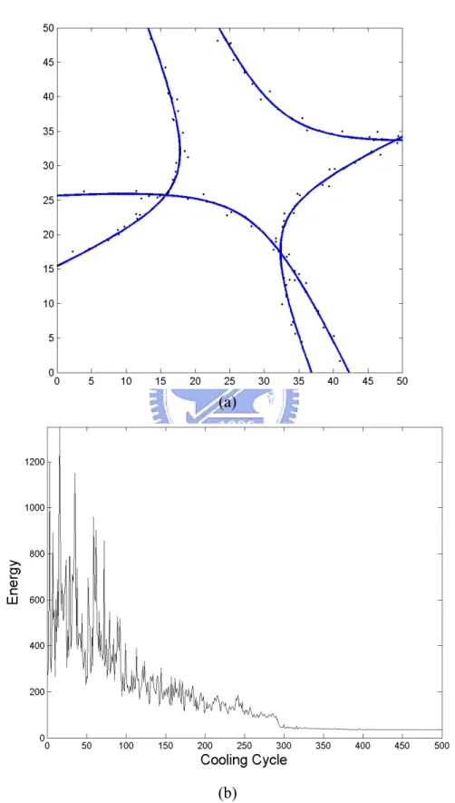
Simulation 2: hyperbolas

Result of detecting hyperbolas are shown in Fig.17 where K = 2. Patterns are with

Gaussian noise N(0, 0.5)×N(0, 0.5). Figures of energy vs. cooling cycles are also shown.

(a)

(b)

Fig.17. Detection of hyperbolas − (a): 2 hyperbolas with noise. (b): error plot of (a)

24

(a)

(b)

Fig.18. Detection of hyperbolas − (a): 2 hyperbolas with noise. (b): error plot of (a)

25

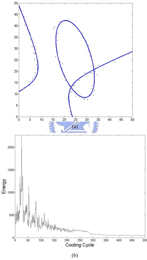
Simulation 3: an ellipse and a hyperbola

Result of detecting ellipses and hyperbolas are shown in Fig.19. Patterns are with

Gaussian noise N(0, 0.5) × N(0, 0.5). Figures of energy vs. cooling cycles are also shown.

(a)

(b)

Fig. 19. Detection of ellipses and hyperbolas − (a): 1 ellipse and 1 hyperbola with

26

Simulation 4: a line and an ellipse

Result of detecting ellipses and hyperbolas are shown in Fig. 20 where K = 2.

Pattern are with Gaussian noise N(0, 0.5) × N(0, 0.5). Figures of energy vs. cooling cycles are also shown.

(a)

(b)

Fig. 20. Detection of ellipses and hyperbolas − (a): 1 ellipse and 1 hyperbola with

27

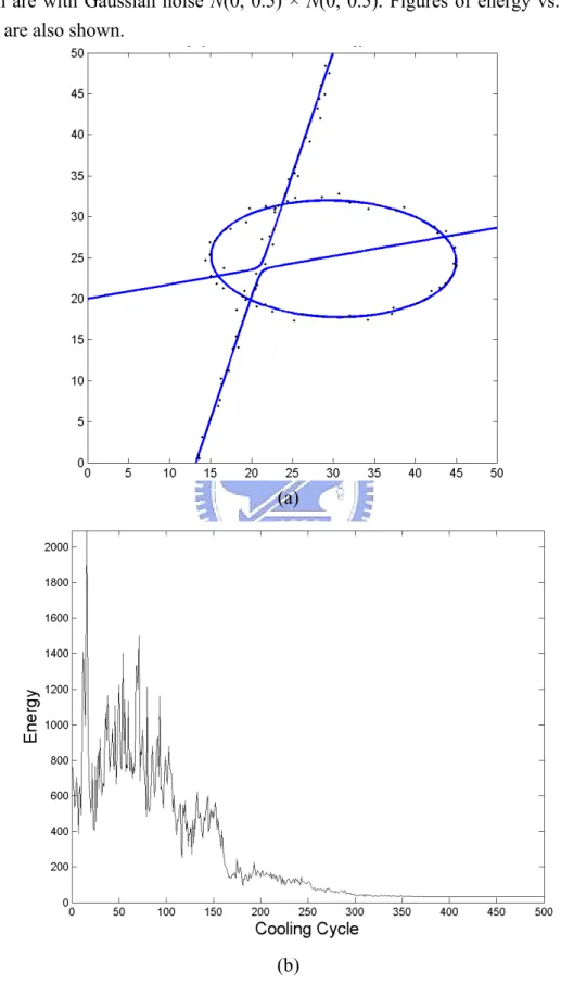
Simulation 5: a line and a hyperbola

Result of detecting ellipses and hyperbolas are shown in Fig. 21 where K = 2.

Patterns are with Gaussian noise N(0, 0.5) × N(0, 0.5). Figures of energy vs. cooling cycles are also shown.

(a)

(b)

Fig.21. Detection of line and hyperbola − (a): 1 line and 1 hyperbola with noise. (b):

28

Simulation 6: two lines

Detected line patterns in Fig. 20 and Fig. 21 have parameter f = 0.245 and f =

0.065 respectively, but the ideal result is f = 0. To make detections more precise, we can put a constraint, f = 0, on detection of lines. Fig.22 and Fig.23 show the result of

detecting lines data are also disturbed by Gaussian noise N(0, 0.5). In Fig. 22, two

lines are crossing at (0, 0). Since asymptotes of a hyperbola are two crossing lines, we can set K = 1 for Fig.22. In Fig.23, we set K = 2, so two additional lines appear.

29

(a)

(b)

Fig.22. Detection of lines by setting f = 0 − (a): 2 lines with noise. (b): error plot of (a) with cooling cycles.

30

(a)

(b)

Fig.23. Detection of lines by setting f = 0 − (a): 2 lines with noise. (b): error plot of (a) with cooling cycles.

31

4.2 Detection of North-South Opening Hyperbolas

North-South opening hyperbolas have the properties a < 0, b > 0, and θ = 0 in (5). We put these constraints in the algorithm to meet the properties. The algorithm used

here is just for North-South opening hyperbola. The detected parameter vector pk =

[mk,x, mk,y, ak, bk, fk]T.

In the initial step, mk,x and mk,y are randomly distributed over (0, 50), ak = -1, bk =

1, and fk = 0 for hyperbolic pattern detection. The cooling function is as (9) with a

high enough temperature, Tmax = 500. We have 100 trials in the same temperature.

The temperature decreases 500 times to T = 0.0209, and this temperature is low enough. Constants αm = 1, αab = 1, and αf = 2.

Fig. 24 and Fig. 25 show the results of North-South opening hyperbolic pattern detection, where Fig. 24 (a) has 187 points and Fig. 25 (a) has 148 points. Each data is with Gaussian noise N(0, 0.5) × N(0, 0.5).

32

(a)

(b)

Fig. 24. Detection of hyperbolas − (a): 2 hyperbolas with noise. (b): Corresponding plot of error vs. cooling cycles of (a).

33

(a)

(b)

Fig. 25. Detection of hyperbolas − (a): 2 hyperbolas with noise. (b): Corresponding plot of error vs. cooling cycles of (a).

34

4.3 Determination of the Number of Patterns

In HTNN [8], the number of patterns was chosen by comparing the results from different number of patterns. Here we propose a method to determine the number of patterns, K, in the image. We define the detection error as

∑

where N is the number of input points. Equation (19) implies that the detection error is the average of the minimum distance from N points to their nearest patterns. Algorithm runs from pattern number K = 1, 2, …, until the detection error has a minimum and no improvement or lower than a threshold. At that time, the best choice of K is determined. Fig. 26 has three circles and shows the result of getting K automatically. In Fig. 26 (e), the detection error greatly decreases and no significant improvement after K = 3. So we choose K = 3. Table II lists the detection error in Fig. 26 (a)-(d).

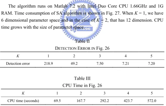
The algorithm runs on Matlab 7.2 with Intel Duo Core CPU 1.66GHz and 1G RAM. Time consumption of SA algorithm is shown in Fig. 27. When K = 1, we have 6 dimensional parameter space and in the case of K = 2, that has 12 dimension. CPU time grows with the size of parameter space.

Table II

DETECTION ERROR IN Fig. 26

K 1 2 3 4 5

Detection error 218.9 49.2 7.50 7.21 7.20

Table III CPU Time in Fig. 26

K 1 2 3 4 5

35

(a) (b)

(c) (d)

(e) (f)

Fig. 26. Determination of number of patterns K. (a): K=1. (b): K=2. (c): K=3. (d): K=4. (e): K=5. (f): Detection error of (a), (b), (c), (d) and (e).

36

37

4.4 Seismic Applications on Simulated data

Experiments on simulated one-shot seismogram have two cases: horizontal reflection layer and dipping reflection layer. Two lines are the asymptote of the hyperbola [3]-[5], and the asymptote is a hyperbola with the same shape but size zero. So a line can be treated as a hyperbola. Here, we use the algorithm just for North-South opening hyperbolas.

Fig. 28 is the simulated horizontal reflection layer where the depth of the

reflection layer is 500m and the velocity of the p-wave in the sedimentary rock is about 2,500m/sec [6]. There are 65 receiving stations on both side of explosion with 50m between each others. The sampling interval is 0.004 sec. The impulse response is 25 Hz Ricker wavelet. Reflection coefficient is 0.2 and noise is band-passed noise, 10.2539Hz ~ 59.5703Hz, with uniform distributed over (-0.2, 0.2).

Fig. 29 (a) shows a one-shot seismogram from horizontal reflection layer in Fig. 28. The horizontal axis in Fig. 29 is the trace number and the vertical axis stands for time t. The one-shot seismogram is first preprocessed by envelope processing in Fig. 29 (b) and thresholding [7] in Fig. 30 with the threshold 0.15. The image size is 512 × 65 where the origin is on the top-left corner with horizontal x-axis and vertical y-axis. The points are then used as the input to the parameter detection system.

The initial parameter mk,x and mk,y are random between 0 and 50, ak = −1, bk = 1,

and fk = 1. The cooling function is as (9) with a high enough temperature, Tmax = 600. There are Nt = 100 trials in a temperature. The temperature decreases 500 times. Constants αm = 1, αab = 0.5, and αf = 5. Since lines of direct wave is asymptotes of a

hyperbola, we set f1 = 0. The result and the error plot are shown in Fig. 31 (a) and (b).

2 k Ground

O’

Receiving station

Reflection wave

Horizontal reflection layer

1

38

(a)

(b)

Fig. 29. Simulated seismic patterns − (a): Simulated one-shot seismogram (horizontal reflection layer). (b): After envelope processing.

39

(a)

(b)

Fig. 30. (a): Result of thresholding from Fig. 29 with the threshold 0.15. The origin is at the top-left corner. (b): Detected peak from (a).

40

(a)

(b)

Fig. 31. Detection of seismic patterns in Fig. 29 − (a): Detection result. (b): Error plot with the cooling cycles.

41

1 2 Ground

Dipping reflection layer

k O

O’

Receiving station Reflection wave

Fig. 32. Illustration of dipping reflection layer.

Fig. 32 illustrates the reflection layer, where the dipping angle is 10° and the depth of the reflection layer is 500m and the velocity of the p-wave in the sedimentary rock is about 2,500m/sec [6]. There are 65 receiving stations on both side of explosion with 50m between each others. The sampling interval is 0.004 sec. The impulse response is 25 Hz Ricker wavelet. Reflection coefficient is 0.2 and noise is band-passed noise, 10.2539Hz ~ 59.5703Hz, with uniform distributed over (-0.2, 0.2). Fig. 33 (a) is the simulated one-shot seismogram. Fig. 33 (b) shows the envelope. Fig. 34 (a) is the result of threshold with the threshold 0.15 and Fig. 34 (b) plots the detect peaks.

Points in Fig. 34 (b) are the inputs to the algorithm. The initial parameters mk,x and mk,y are random between 0 and 50, ak = −1, bk = 1, and fk = 1. The cooling function is

as (9) with a high enough temperature, Tmax = 600. There are Nt = 100 trials in a

temperature. The temperature decreases 500 times. Constants αm = 1, αab = 0.5, and αf

= 5. Number of patterns is K = 2, and we set f1 = 0 for line patterns of direct wave. Fig.

35 (a) is the detection result of Fig. 34 (b) and Fig. 35 (b) is the corresponding error plot.

42 (a)

(b)

Fig. 33. Simulated seismic patterns − (a): Simulated one-shot seismogram (dipping reflection layer). (b): After envelope processing.

43 (a)

(b)

Fig. 34. (a): result of thresholding from Fig. 33(b) with the threshold 0.15. The original is at the top-left corner. (b): detected peak from (a).

44 (a)

(b)

Fig. 35. Detection of seismic patterns in Fig. 33 − (a): Detection result. (b): Error plot with the cooling cycles.

45 Table IV

Detected parameters in Fig. 31 (a) in image space 512×65

mx my a b f

Direct wave 33.01 8.21 -5.031 0.198 0 (preset)

Reflection wave 32.95 40.09 -4.412 0.226 1040.99

Table V

Detected parameters in Fig. 35(a) in image space 512×65

mx my a b f

Direct wave 33.00 8.96 -5.00 0.199 0 (preset)

46

4.5 Seismic Applications on Real Seismic Data

The system is also applied to detect direct wave and reflection wave in real seismic data. We obtain data from Seismic Unix System developed by Colorado School of Mine [5].

The real data with the size 3100×48 showed in Fig. 36 (a) is from Canadian Artic, which has 48 traces and 3100 samples per trace with sampling interval 0.002 seconds. The horizontal axis is the trace number and the vertical axis is time t.

After envelope and threshold preprocessing [7], Fig. 36 (b) shows the result of envelope and Fig. 37 (a) shows the result of thresholding with the threshold 0.15. The result of peak detection is in Fig. 37 (b). We only choose points with y < 700 which includes points from direct wave, first reflection wave and second reflection wave as in Fig. 38 (a) where there are 88 points. Detected curves are plotted in Fig. 38 (b) with

K = 3 and we preset f1 = 0. Here, the initial parameters mk,x and mk,y are random

number between 0 and 50, ak = −1, bk = 1, and fk = 0. The cooling function is as (9)

with a high enough temperature, Tmax = 1,000. There are Nt = 100 trials in a

temperature, and the temperature decreases 500 times. Constants settings: αm = 1, αab

= 0. 5, and αf = 10.

Since the second reflection wave is not a hyperbola in theory [3], we remove the points from the second-layer reflection wave. That is, we remove the points nearest to the bottom pattern in Fig. 38 (b). Remaining 65 points are plotted in Fig. 39 (a). We redo the experiment, and this time K = 2. Fig. 39 (b) shows the result. The detected parameters in Fig. 38 (b) and Fig. 39 (b) are listed in Table VI and Table VII.

Table VI

Detected parameters in Fig. 38 (b) with fixed f1 = 0 in image space 3100×48

mx my a b f

Direct wave 24.48 8.59 -25.69 0.038 0 (preset)

Reflection wave 24.83 28.83 -22.91 0.044 2,441.7

47 Table VII

Detected parameters in Fig. 39 (b) with fixed f1 = 0 in image space 3100×48

mx my a b f

Direct wave 24.53 11.20 -25.59 0.039 0 (preset)

Reflection wave 24.62 -2.81 -24.13 0.041 2,978.05

As mentioned in [3]-[5], two lines of direct wave is a pair of asymptotes of the hyperbola and a pair of asymptotes is a hyperbola with size zero. From the detected parameters in Table VIII, we obtain the equation of the direct wave

) 20 . 11 ( 039 . 0 ) 53 . 24 ( 59 . 25 0 ) 20 . 11 ( 039 . 0 ) 53 . 24 ( 59 . 25 2 2 2 − = − ⇒ = − + − − y x y x (20) Rearrange (20) and take square root on both sides, the equations of two lines in image space are 3019 . 126 1975 . 0 0587 . 5 8779 . 121 1975 . 0 0587 . 5 = + = − y x y x (21)

48

(a)

(b)

Fig. 36. Experiment on real data -- (a): Real seismic data from Canadian Artic. (b):

49

(a)

(b)

50

(a)

(b)

Fig. 38. Experiment on real data -- (a): Choose peak with y < 700. (b): Detection

51

(a)

(b)

Fig. 39.Experiment on real data -- (a): Remove points nearest to the bottom pattern.

52

(a)

(b)

Fig. 40. Plot detected curve on the original data -- (a): Detection result from Fig. 38

53

The other real data is Gulf of Cadiz’s seismic data. There are 48 traces and 2050 samples in a trace with sampling interval 0.004 seconds. Fig. 41 (a) shows the real data. The horizontal axis is the trace number and the vertical axis is time t.

After envelope and threshold preprocessing [7], Fig. 41 (b) shows the envelope and Fig. 42 shows the thresholding result with threshold 0.5. The detected peak in Fig. 42 are plotted in Fig. 43 (a) where there are 66 points and the size of image is 2050×48, where the horizontal axis is x and the vertical axis is y. The initial parameters mk,x and mk,y are random number between 0 and 50, ak = −1, bk = 1, and fk

= 0. The cooling function is as (9) with a high enough temperature, Tmax = 1,000.

There are Nt = 100 trials in a temperature. The temperature decreases 500 times. Constants settings: αm = 1, αab = 0.5, and αf = 10. Number of patterns is K = 2. The

detection result is in Fig. 43 (b).

Since the points nearest to the pattern around y = 800 are from second-layer reflection wave. In theory, the second-layer reflection wave is not a hyperbola [3]. We remove those points and remaining 48 points are plotted in Fig. 44 (a). Fig. 44 (b) shows the detection result and Fig. 45 plots the detected curve in the original data. Table VIII and Table IX list the detected parameters in image space in Fig. 43 (b) and Fig. 44 (b).

Table VIII

Detected parameters in Fig. 43 (b) in image space 2050×48

mx my a b f Reflection wave 44.57 187.84 -6.93 0.144 2,116.8 Second-layer reflection wave 21.64 56.27 -25.13 0.040 12,537.7 Table IX

Detected parameters in Fig. 44 (b) in image space 2050×48

mx my a b f

54

(a)

(b)

Fig. 41.Experiment on real data -- (a): Real seismic data from Gulf of Cadiz. (b): Plot

55

(a)

Fig. 42.Experiment on real data – Thresholding result of the envelope in Fig. 41 (b)

56

(a)

(b)

Fig. 43. Experiment on real data -- (a): Detected peak from Fig. 42. (b): Detection

57

(a)

(b)

Fig. 44.Experiment on real data -- (a): Remove points nearest to the pattern around y

58

59

Chapter 5

Conclusions and Discussions

5.1 Conclusions

This paper is about a proposed system, which adopted the simulated annealing algorithm to detect patterns such as lines, circles, ellipses, and hyperbolas by finding their parameters in an unsupervised manner and global minimum fitting error related to points in an image. The iterative adjustment requires less memory space. Also, we define the distance from a point to a pattern and this makes the computation feasible, especially for hyperbola. Using four steps to adjust parameters from center, shape, angle to the size of the pattern can get fast convergence. Based on the average minimum distance from points to patterns, we have proposed a method to determine the number of patterns automatically. Experimental results on the detection of line, circle, ellipse, and hyperbola in images are successful. The detection results of line pattern of direct wave and hyperbolic pattern of reflection wave in one-shot seismogram are good, and can improve seismic interpretations and further seismic data processing.

5.2 Discussions

Parameter settings. In the cooling schedule, the value of Tmax, and Nt, are set prior.

For a trial which includes a change of center, a change of b and a, a change of θ, and a change of f for every pattern, there are three possible results to accept or reject the change determined by Metropolis criterion:

1. The new parameter has smaller error and it is accepted. 2. The new parameter has larger error and it is still accepted. 3. The new parameter has larger error and it is rejected.

The determination of Tmax, we considered the accept ratio of the larger-error trials. If the Tmax is not high enough, the trial with larger error will almost reject, that is, it always accept trial with smaller error, so it is possible to reach local minimum. Fig. 46 shows this situation, where Tmax = 1,500 iterations, initial center (0,0), a = 1, b = 1, θ

60

= 0, and f = 1. Fig. 47 shows the result when Tmax = 10. In Fig. 47 (b), the accept ratio of canter, angle, and size has increased and shows the good result for this simple

example. Fig. 48 show the result when Tmax = 100,000. After 500 iterations, T = 4.1,

but this temperature is not low enough and the high accept ratio of larger-error parameters results in the instability. To solve this problem, we can increase the number of iterations to 1,000 and show the result in Fig. 49. This still shows good

result, but it takes more time. In conclusions, for temperature Tmax, we have to choose

a high enough temperature that gives a high accept ratio of larger-error parameters. Besides, we need many enough iterations to cool the temperature to ensure stability.

Also we find the setting of Tmax is proportional to the scale of input points. In Fig.

47, Tmax = 10 provides good result. In Fig. 50, we enlarge the scale of data by two.

Fig. 50 (a) with Tmax = 10 cannot give good result, but Fig. 50 (a) with Tmax = 100 can

give good result. In our simulation experiments, we choose Tmax = 500 and 500

iterations to ensure high enough initial temperature and lower final temperature T ≈ 0.02.

As for Nt, if trials are not many enough, we cannot get good result. Larger Nt takes more time but gives more chances. So we can have as many trials as possible if the computational power is strong enough. Fig. 51 shows too few trials cannot provide good result and for this simple example we need only Nt = 10 to obtain a good result.

61

(a)

(b)

Fig. 46. Illustration of low initial temperature Tmax: (a) Detection result of Tmax = 1. (b) Accept ratio of larger-error parameters.

62

(a)

(b)

Fig. 47. Illustration of low initial temperature Tmax: (a) Detection result of Tmax = 10. (b) Accept ratio of larger-error parameters.

63

(a)

(b)

Fig. 48. Illustration of high initial temperature Tmax: (a) Detection result of Tmax = 100,000. (b) Accept ratio of larger-error parameters.

64

(a)

(b)

Fig. 49. Illustration of high initial temperature Tmax with more iterations: (a) Detection result of Tmax = 100,000. (b) Accept ratio of larger-error parameters.

65

(a)

(b)

Fig. 50. Enlarge the scale of points by two: (a) Detection result of Tmax = 10. (b)

66

(a)

(b)

Fig. 51. Relationship between Nt and detection result Tmax = 500: (a) Detection result

of Nt= 1. (b) Detection result of Nt = 10.

Time consumption. As for the time consumption, Table III shows that the CPU

time is proportional to the number of patterns or the number of parameters. The larger number of parameters, the algorithm takes more time to obtain the solution.

Memory requirement. For traditional HT, it needs an accumulation matrix. The

67

the higher precision, the larger accumulator matrix is needed. On the other hand, SA algorithm for parameter detection needs only memories for the original parameters and the trials parameters. This depends on the number of patterns K. Furthermore, the parameters can be presented by SA algorithm with high precision since we do not need to quantize the parameter space as in the traditional HT.

Preprocessing. In seismic application, we have no constraint on the center.

However, for ideal case, the hyperbola has the center on x-axis, i.e. t = 0. In simulated seismic data, we can find that the center does not lie on the x-axis, since convolution produces a shift. So preprocessing is quite critical. Wavelet and deconvolution processing may be needed in the preprocessing to improve the detection result.