橢圓介面方程的數值研究

國

立

交

通

大

學

應用數學學系

碩 士 論 文

橢圓介面方程的數值研究

Numerical Study of Elliptic Interface Problems

研 究 生：胡偉帆

指導教授：賴明治 教授

橢圓介面方程的數值研究

Numerical Study of Elliptic Interface Problems

研 究 生：胡偉帆 Student：Wei-Fan Hu

指導教授：賴明治 Advisor：

Ming-Chih Lai

國 立 交 通 大 學

應 用 數 學 系

碩 士 論 文

A Thesis

Submitted to Department of Department of Applied Mathematics College of Science

National Chiao Tung University in partial Fulfillment of the Requirements

for the Degree of Master

in

Applied Mathematics July 2008

橢圓介面方程的數值研究

學生：胡偉帆 指導教授：賴明治

國立交通大學應用數學系（研究所）碩士班

摘要

本文利用新的任意高階精度內嵌介面方法計算橢圓界面方程，並且應用

至有介面的熱方程問題，我們推導出四階精度公式和測試數值結果。本方法

的優點是容易應用於其他問題並且使數值精確度有顯著的改善。

Numerical Study of Elliptic Interface Problems

Student: Wei-Fan Hu Advisor: Ming-Chih Lai

Department (Institute) of Applied Mathematics

National Chiao Tung University

Abstract

In this thesis, we introduce an arbitrary high-order immersed interface method for

solving elliptic equations and apply it to solve heat equation with interface. We

have derived fourth-order scheme and tested in examples. The advantage of

method in this thesis is easy to apply to other problems, such as two-phase flow

and leads to a significant improvement in accuracy.

誌 謝

本篇論文的完成，首先要感謝我的指導老師－賴明治教授。在老師指點下，讓我逐

漸熟悉了數值偏微分方程以及科學計算的方法。使我在數值方法與科學計算這片領中，

找到我的興趣已經研究做出的成就感。老師不只引導我學習應有的態度，並且也教導我

們做人的道理，相信在往後的人生的道路上將會受用無窮。除了指導老師外，科學計算

研究室的其他學長們也給我不少助力。感謝曾昱豪學長與曾孝捷學長，在我剛進入這片

領域時給我引導，教導我許多研究上的知識。感謝陳冠羽學長，總是耐心地回答我各式

各樣的疑難雜症，讓我在課業上以及生活上有極大的幫助。

在口試論文期間，承蒙黃聰明教授、王偉仲教授與吳金典助理教授費心審閱並提供

許多寶貴意見，使得本論文更加完備，學生永銘記在心。

除了研究外，我也要感謝其他同屆的同學們，除了課業上的討論外，閒暇之餘能與

他們閒話家常，一起運動，交換各種心得，讓我的研究生生活充滿樂趣。

最後，我要感謝我的家人，沒有他們的鼓勵與支持，我無法順利地完成學業。願與

他們，以及所有在我周圍關心我的人，一同分享此篇論文完成之喜悅與榮耀。

目 錄

中文提要

………

i

英文提要

………

ii

誌謝

………

iii

目錄

………

iv

一、

Introduction………

1

二、

Basic Definition ………

2

2.1

Cartesian Grid………

2

2.2

Jump Conditions ………

3

2.2.1 One dimension ………

3

2.2.2 Two dimensions………

3

2.3

Level Set Function………

4

三、

One-Dimensional Elliptic Interface Problems ………

4

3.1

Difference Formulas for

at Irregular Points ……

5

3.1.1 Difference Formulas with Four-point Stencil

…

6

3.1.2 Irregular Point Located at Right Side of Interface ………

8

3.2

Difference Formulas with a General

Grid Stencil…

10

3.3

Numerical Results………

12

四、

Two-Dimensional Elliptic Interface Problems………

14

4.1

Poisson Equation with Interface ………

15

4.2

Elliptic Equation with Interface ………

16

4.3

Numerical Results………

17

4.3.1 Poisson Equation ………

17

4.3.2 Elliptic Equation ………

20

4.3.3 Application of Heat Equation ………

22

五、

Conclusion………

24

1

Introduction

In this thesis, we propose a numerical method for solving elliptic equation with interface in the following

∇ · (β∇u) − κ(x)u(x) = f (x).

The equation is defined in a simple region with a uniform Cartesian grid and the coefficient β and κ can be discontinuous across interface. From this equation, we can derive two jump conditions:

[u] and [βun].

We will use these two natural jump conditions as known in our method. In solving problems with interface, since the derivative terms may have jump discontinuities, we cannot use finite difference directly. One intuitional way is that use one-sided difference formula at grid points near the interface, but it will lead the linear system insolvable because of the singularity of the matrix. The Immersed Interface Method (IIM) has been developed as a sharp interface method which can accurately capture discontinuities in the solution.

The first IIM paper was developed by Leveque and Li[3]. The original IIM uses three points to discrete the derivative term in equation to maintain the compact structure of matrix. In this thesis we use four points to reduce the complex work in original IIM. Mayo used the similar idea earlier in [9] on the fast solution of the Poisson and biharmonic equations. There are also lots of treatments for the immersed interface problems[2, 4, 5, 6, 7, 8].

The term “immersed interface” has been used since the method is mo-tivated by Peskin’s “immersed boundary method” (IBM). The equation is discretized by a standard finite difference method in a fixed Cartesian grid and the singular delta function is substituted by an approximated smooth function spanning a few grid cells. But this method is of first-order accuracy. First of all, We give some basic definition and useful tools in Sec. 2 and secondly we introduce the singularity into a finite difference scheme in Sec. 3. Finally, we test some examples to show our work in Sec. 4.

2

Basic Definition

2.1

Cartesian Grid

We usually assume that the domain Ω is a rectangle for interface problems. For example, Ω = [a, b] in one-dimensional case, Ω = [a, b] × [c, d] in two-dimensional case, and Ω = [a, b] × [c, d] × [r, s] in three-two-dimensional case. The Cartesian grid can be represented by

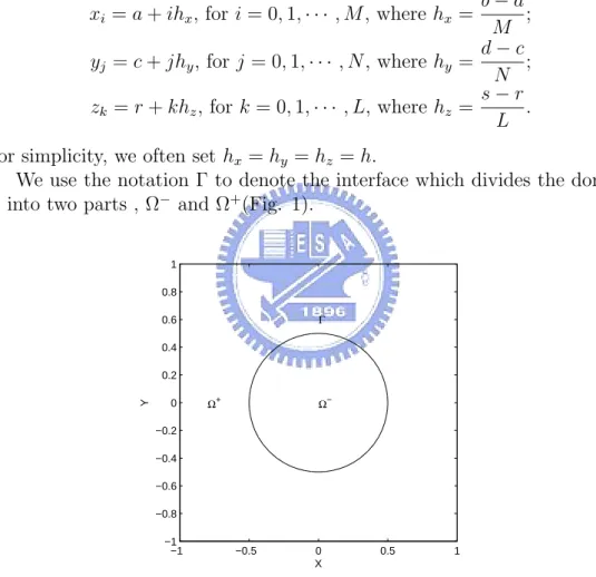
xi = a + ihx, for i = 0, 1, · · · , M , where hx = b − a M ; yj = c + jhy, for j = 0, 1, · · · , N , where hy = d − c N ; zk = r + khz, for k = 0, 1, · · · , L, where hz = s − r L .

For simplicity, we often set hx = hy = hz = h.

We use the notation Γ to denote the interface which divides the domain

Ω into two parts , Ω− _{and Ω}+_{(Fig. 1).}

Ω− Ω+ Γ X Y −1 −0.5 0 0.5 1 −1 −0.8 −0.6 −0.4 −0.2 0 0.2 0.4 0.6 0.8 1

2.2

Jump Conditions

2.2.1 One Dimension

Given a piecewise smooth function u(x) that can have the finite jump across interface. We give a notation defined as following:

u±_{(α) = lim}

ε→0+u(α ± ε). (1) The jump condition at x = α in x-direction is defined by

[u(α)]x = u+(α) − u−(α). (2)

For simplicity, we often omit that u±_{(α) = u}± _{and use the notation [u] to}

define the jump condition across interface. The subscript of [ ]x may be little

strange but it will be useful in extension to two dimensions.

2.2.2 Two Dimensions

Given a point X = (X, Y ) on the interface Γ. The limiting values of u(X)

and un(X) are defined as

u±(X) = lim ε→0+u(X ± εn), (3) u±_n(X) = ∂u ∂n ± (X) = ∇u±(X) · n, (4)

where n = (n1, n2) is the outward unit normal vector. Then the jump

con-ditions on interface are defined as

[u] = u+_{− u}− _{and [u}

n] = u+n − u−n. (5)

We should be able to figure out “+” and “−” sides without confusion. It’s

also useful to define [ ]x, the jump in x-direction and [ ]y, the jump in

y-direction as

[u]x = u(X+, Y ) − u(X−, Y ) and [u]y = u(X, Y+) − u(X, Y−). (6)

From (5) and (6), we can easily obtain

[u]x = sgn(n1)[u] and [u]y = sgn(n2)[u]. (7)

2.3

Level Set Function

In this approach, an interface is represented by the zero level set of function

φ. The following is the definition of φ on whole domain: φ(x) < 0 if x ∈ Ω−

φ(x) = 0 if x ∈ Γ φ(x) > 0 if x ∈ Ω+

We call φ is a signed distance function if φ(x) is the distance from x to the interface. We will use re-initialization process[10] to modified level set function into signed distance function so that use φ to define the outward unit normal vector n by

n = ∇φ

|∇φ|, (8)

and the curvature κ by

κ = ∇ · n = ∇ · µ ∇φ |∇φ| ¶ . (9) If X is on the interface but is not a grid point, we can still compute them by the interpolation method using specific points from the four corners of the rectangle that contains X.

3

One-Dimensional Elliptic Interface

Prob-lems

In this section, we discuss with one-dimensional elliptic equation. Extending to two-dimensional elliptic equations is using dimension by dimension. The key idea of IIM is to avoid grid generation by correcting finite difference in the neighborhood of the interface. We only show the work about discrete form of (d2u/dx2₎

j. The discrete form of (du/dx)j can be easily obtained by

the same way.

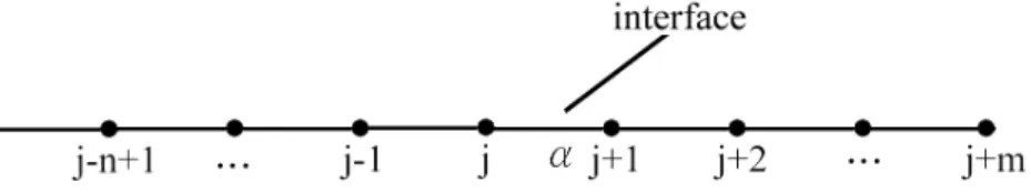
Assume the interface is located at x = α(Fig. 2). Let

σ = α − xj

h . (10)

Figure 2: Uniform grid with interface located at x = α

The two jump conditions involving u and ux can be obtained from the

original elliptic equation. A general jump conditions across the interface can be written as [γu]x = γ+u+− γ−u−= A (11) and · βdu dx ¸ x = β+du dx + − β−du dx − = B. (12)

As mention in Sec. 2.2, the superscripts “+” and “−” represent the variables at the right and left side of the interface, respectively.

There are two kinds of grid points. One is called a regular point if the finite difference formula at this point only involves grid points on the same side of the interface. Otherwise, it is an irregular point. If the gird point i is a regular point, we use standard finite difference directly. For example:

µ d2u dx2 ¶ j = uj−1− 2uj + uj+1 h2 + O(h 2_{) (13)} or µ d2_u dx2 ¶ j

= −uj−2+ 16uj−1− 30uj + 16uj+1− uj+2

12h2 + O(h

4_{). (14)}

These two difference formulas can be easily obtained by the Taylor expansion.

3.1

Difference Formula for d

u/dx

_{at Irregular Points}

Finite difference approximations for d2u/dx2 _{at the irregular point j are}

considered by using a stencil of n points on the left side of interface and m points on the right(Fig. 2).

3.1.1 Difference Formulas with Four-point Stencil (n = m = 2) In this section, we discuss the case n = m = 2. Let

µ d2u dx2 ¶ j ≈ d−1uj−1+ d0uj+ d1uj+1+ d2uj+2+ dAA + hdBB h2 . (15)

Thus, we have to determine dks and the correction term on the right hand

side of Eq. (15). By using the Taylor expansion at x = α−_{, we have}

u(x) = u(α−) + u 0_(α−₎ 1! (x − α −_{) +} u00(α−) 2! (x − α −₎2_{+ · · · . (16)}

Let x = xj−1 in Eq. (16), then we have

uj−1 = u(α−) + u0_(α−₎ 1! (xj−1− α −_{) +} u00(α−) 2! (xj−1− α −₎2_{+ · · · . (17)}

Take ε → 0, Eq. (17) becomes

uj−1 = u−− µ du dx ¶₋ (1 + σ)h + 1 2! µ du dx ¶₋ (1 + σ)2_h2_{+ · · · . (18)} Similarly, uj = u−− µ du dx ¶₋ σh + 1 2! µ du dx ¶₋ σ2_h2 _{+ · · · , (19)} uj+1= u++ µ du dx ¶₊ (1 − σ)h + 1 2! µ du dx ¶₊ (1 − σ)2h2+ · · · , (20) uj+2= u++ µ du dx ¶₊ (2 − σ)h + 1 2! µ du dx ¶₊ (2 − σ)2_h2_{+ · · · . (21)}

Substituting Eqs. (11) and (12) into Eq. (20) and (21), we have

uj+1 = A γ+ + (1 − σ)hB β+ + cγu −_{+ c} β(1 − σ)h µ du dx ¶₋ + 1 2!(1 − σ) 2_h2 µ d2u dx2 ¶+ + · · · , (22) uj+2 = A γ+ + (2 − σ)hB β+ + cγu −_{+ c} β(2 − σ)h µ du dx ¶₋ + 1 2!(2 − σ) 2_h2 µ d2_u dx2 ¶+ + · · · , (23) where cγ = γ− γ+ and cβ = β− β+.

Substituting Eqs. (18), (19), (22), and (23) into Eq. (15) leads to µ d2u dx2 ¶ j = 1 h2 Ã a1u−+ a2 µ du dx ¶₋ h + a3 µ d2u dx2 ¶− h2_{+ a} 4 µ d2u dx2 ¶+ h2 + a5A + a6Bh + O(h3) ! . (24) Since µ d2u dx2 ¶ j = µ d2u dx2 ¶− + O(h), (25)

we take ai = 0 for i = 1, 2, 4, 5, 6 and a3 = 1. From Eqs. (24) and (25), we

can conclude that the (d2_u/dx2_{) at irregular points is O(h). To determine}

dks, it is necessary to solve the linear system equation as follows

            1 1 cγ cγ 0 0 −(1 + σ) −σ (1 − σ)cβ (2 − σ)cβ 0 0 (1 + σ)2 _σ2 _{0 0 0 0} 0 0 (1 − σ)2 _{(2 − σ)}2 _{0 0} 0 0 1 1 γ+ ₀ 0 0 (1 − σ) (2 − σ) 0 β+                         d1 d0 d1 d2 dA dB             =             0 0 2 0 0 0             . Therefore, we get d−1 = 1 D{cγ(3σ − 2σ 2_{) − c} β(−2 + 3σ − σ2)}, d0 = 1 D{cγ(−3 − σ + 2σ 2_{) − c} β(2 − 3σ + σ2)}, d1 = 1 D{4 − 4σ + σ 2_{}, (26)} d2 = 1 D{−1 + 2σ − σ 2_}, dA = 1 γ+_D{−3 + 2σ}, dB = − 1 β+_D{2 − 3σ + σ 2_}, where 1 _{2 3 2 3}

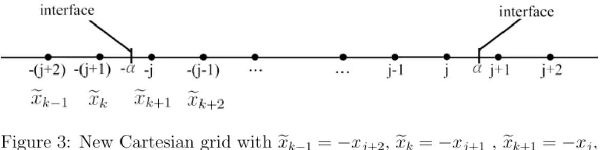
Figure 3: New Cartesian grid with exk−1 = −xj+2, exk = −xj+1 , exk+1 = −xj,

and exk+2 = −xj−1.

Clearly, dks are functions of σ and jump parameters: γ+, β+, cγ, and cβ.

Finally, we’ve determined all dks. Eq. (15), together with Eq. (26), is an

explicit difference formula for O(h) approximation to (d2u/dx2₎

j. Moreover,

it shows that the current formula at irregular points does not have singularity, even for the special cases of Γ coinciding with σ = 0 or σ = 1.

We can obtain (du/dx)j by the same way. The general formulas for first

and second derivatives terms are µ du dx ¶ j = (d−1− 2)uj−1+ (d0+ 2)uj+ d1uj+1+ d2uj+2+ dAA + hdBB 2h + O(h), (27) µ d2u dx2 ¶ j = d−1uj−1+ d0uj + d1uj+1+ d2uj+2+ dAA + hdBB h2 + O(h), (28)

where dks are the same in Eq. (26).

3.1.2 Irregular Point Located at Right Side of Interface

The finite difference formulas at grid point j + 1 can be obtained from Eqs. (27) and (28). Instead of using the method in previous section, we use the coordinate transformation (Fig. 3).

Let v(x) = u(−x), e γ(x) = γ(−x), e β(x) = β(−x), (29) [eγv]x = eA, [ eβv0_] x = eB,

then the two jump conditions are [eγv]x = lim ε→0+eγ(−α + ε)v(−α + ε) − eγ(−α − ε)v(−α − ε) = lim ε→0+γ(α − ε)u(α − ε) − γ(α + ε)u(α + ε) = γ−_u−_{− γ}+_u+ = −[γu] = −A and [ eβv0_] x= lim ε→0+ e β(−α + ε)v0_{(−α + ε) − eβ(−α − ε)v}0_{(−α − ε)} = lim ε→0+−β(α − ε)u 0_{(α − ε) + β(α + ε)u}0_{(α + ε)} = −β−_u0− _{+ β}+_u0+ = −[βu0] = B.

Consider the derivative of function v defined on the Cartesian grid exk. By

the same thought in Sec. 3.1.1, we can easily obtain µ

d2_v

dx2

¶

(exk) =

d−1v(exk−1) + d0v(exk) + d1v(exk+1) + d2v(exk+2) + dAA + hde BBe

h2 + O(h).

(30)

Note that the dks are functions of σ0, where σ0 = 1 − σ and σ is the same as

Eq. (10). Similarly, all dks are functions of parameters: eγ+ and eβ+, where

e

γ+ _{= γ}− _{and eβ}+ _{= β}−_{. By Eq. (29), we have v}00_{(x) = u}00_{(−x), and then Eq.}

(30) becomes µ d2u dx2 ¶ j+1 = d2uj−1+ d1uj+ d0uj+1+ d−1uj+2− dAA + hdBB h2 + O(h). (31) Similarly, we have µ du dx ¶ j+1 = −d2uj−1+ d1uj + (d0+ 2)uj+1+ (d−1− 2)uj+2− dAA + hdBB 2h + O(h). (32)

3.2

Difference Formulas with a General n + m Grid

Stencil

In this section, we want to obtain arbitrary high order difference formula scheme. The difference formulas at irregular point j for n + m points are considered. In order to get uniform order, we often take n = m. The method we used is matched polynomial interpolation. We only provide the discrete

form of d2u/dx2 _here.

The polynomial on the left side of Γ, interpolating through n grid points can be written as

P−_{(x) =}

−n+1_X

k=0

lk(x)ui+k+ anR(x), (33)

where an is an undetermined coefficient to be decided, and

R(x) =

−n+1_Y

k=0

(x − xi+k). (34)

lk(x) is the Lagrange polynomial, i.e.

lk(x) = −n+1_Y l=0,l6=k (x − xi+l) . −n+1_Y l=0,l6=k (xi+k− xi+l). (35)

Similarly, the polynomial on the right side of Γ, interpolating through m grid points can be written as

P+_{(x) =}

m

X

k=1

rk(x)ui+k+ bmQ(x), (36)

where bm is an undetermined coefficient to be decided, and

Q(x) =

m

Y

k=1

(x − xi+k). (37)

rk(x) is the Lagrange polynomial, i.e.

rk(x) = m Y l=1,l6=k (x − xi+l) . _Ym l=1,l6=k (xi+k− xi+l). (38)

Our thought is that use the relation µ d2_u dx2 ¶ j ≈ µ d2_P−_(x) dx2 ¶ x=xj .

Thus, we only have to determine the unknown an. Once we find an, we can

obtain the difference formula (d2u/dx2₎

j, and then we get (d2u/dx2)j+1 by

the method in Sec. 3.1.2.

Substituting Eqs. (33) and (36) into Eq. (11) leads to

γ+ ( m X k=1 rk(α)ui+k+ bmQ(α) ) − γ− ( −n+1_X k=0 lk(α)ui+k+ anR(α) ) = A. Rearrange the equation above we get

c11an+ c12bm = β1, (39) where c11= −γ−R(α), c12= γ+Q(α), (40) β1 = A − γ+ m X k=1 rk(α)ui+k+ γ− −n+1_X k=0 lk(α)ui+k.

Again, Substituting Eqs. (33) and (36) into Eq. (12) leads to

β+ ( _m X k=1 r0_k(α)ui+k+ bmQ0(α) ) − β− (_−n+1 X k=0 l0_k(α)ui+k+ anR0(α) ) = B. Rearrange the equation above we get

c21an+ c22bm = β2, (41) where c21 = −β−R0(α), c22 = β+Q0(α), (42) β2 = B − β+ m X k=1 r0 k(α)ui+k+ β− −n+1_X k=0 l0 k(α)ui+k.

Solving Eqs. (39) and (41), we have

an= m

X

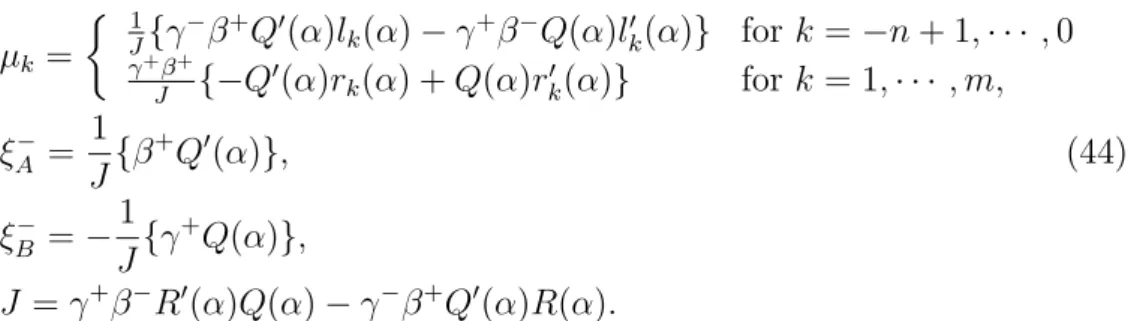
where µk= ½ ₁ J{γ−β+Q0(α)lk(α) − γ+β−Q(α)l0k(α)} for k = −n + 1, · · · , 0 γ+_β+ J {−Q0(α)rk(α) + Q(α)r0k(α)} for k = 1, · · · , m, ξ− A = 1 J{β +_Q0_{(α)}, (44)} ξ− B = − 1 J{γ +_Q(α)}, J = γ+β−R0(α)Q(α) − γ−β+Q0(α)R(α).

In fact, if we take n = m = 2, we will have the same result as present in the previous section.

3.3

Numerical Results

We use four versions of current IIM tested in this thesis. In method C and D, grid points j − 1 and j + 2 are irregular points, but we can treat only j and

j + 1 as irregular points and use fourth-order one-sided difference formula for j − 1 and j + 2.

Methods Order at regular Order at irregular Expected global order

grid points grid points

Method A O(h2_{) O(h) O(h}2₎

Method B O(h2_{) O(h}2_{) O(h}2₎

Method C O(h4_{) O(h) O(h}2₎

Method D O(h4_{) O(h}2_{) O(h}3₎

Table 1: Four immersed interface method

Example 3.1 In this example, we use the IIM to solve the following prob-lem:

d2u

dx2 + κu = βδ(x − α) , x ∈ (−0.5, 0.5), (45)

where κ is discontinuous across the interface located at x = α:

κ(x) =

½

(α1)2 if − 0.5 < x ≤ α,

The boundary condition is

u(−0.5) = u(0.5) = 0. (47) An alternative way to state Eq. (45) requires that u(x) satisfies the equation

d2u

dx2 + κu = 0 , x ∈ (−0.5, α) ∪ (α, 0.5), (48)

excluding the interface located at x = α, together with boundary conditions (47) and two natural jump conditions:

[u]x = 0, (49) · du dx ¸ x = β. (50)

The exact solution is

uex(x) =        β cos(α2α) cos(α1x)

α1cos(α2α) sin(α1α) − α2sin(α2α) cos(α1α) if − 0.5 < x ≤ α,

β cos(α1α) cos(α2x)

α1cos(α2α) sin(α1α) − α2sin(α2α) cos(α1α) if α < x < 0.5.

(51)

Take α = 4/15, β = −40π, α1 = 7π, and α2 = 5π. The jump parameters

are: γ+_{= β}+_{= c} γ = cβ = 1, A = 0, and B = β. −0.5 0 0.5 −8 −6 −4 −2 0 2 4 X Y (a) (b) u ex u −0.5 0 0.5 −3 −2 −1 0 1 2x 10 −5

Figure 4: (a)Comparison of the exact solution uexand the numerical solution

Table 2 shows the maximum-norm errors of four methods, the correspond-ing ratios and orders. Note that in order to compare the grid refinement results with the same conditions, all results are compared between grids N and N/4 because they have the same σ. So the ratio and order are defined as following: Ratio = kEN/4k∞ kENk∞ , Order = log₄ µ kEN/4k∞ kENk∞ ¶ . N σ Method A Method B

kEnk∞ Ratio Order kEnk∞ Ratio Order

20 1/3 9.795371 9.884993 40 2/3 9.537e-1 9.369e-1 80 1/3 2.135e-1 45.875 2.76 2.135e-1 46.79 2.77 160 2/3 5.277e-2 18.073 2.09 5.189e-2 18.05 2.08 320 1/3 1.297e-2 16.466 2.02 1.288e-2 16.39 2.01 640 2/3 3.275e-3 16.112 2.00 3.222e-3 16.10 2.00 N σ Method C Method D

kEnk∞ Ratio Order kEnk∞ Ratio Order

40 2/3 3.673e-1 3.762e-1

80 1/3 1.269e-2 8.797e-3

160 2/3 2.709e-3 135.5 3.54 1.016e-3 369.9 4.27

320 1/3 2.198e-4 57.72 2.92 2.521e-5 348.9 4.22

640 2/3 1.255e-4 21.57 2.21 1.112e-5 91.44 3.26

Table 2: Comparison of numerical errors

4

Two-Dimensional Elliptic Interface

Prob-lems

We use a dimension by dimension approach to solve the two-dimensional problems. To compute two-dimensional problems, the grid points are classi-fied into four categories in x-direction:

1. Regular point;

2. Irregular point located on left side of interface; 3. Irregular point located on right side of interface; 4. Irregular point near two interface.

The definition in y-direction is similar to x-direction.

For regular point away from the interface, the derivatives with respect to

x and y are approximated by standard central difference:

µ d2u dx2 ¶ i,j =     

ui−1,j − 2ui,j+ ui+1,j

h2 + O(h2)

−ui−2,j + 16ui−1,j − 30ui,j + 16ui+1,j− ui+2,j

12h2 + O(h4) (52) µ d2_u dy2 ¶ i,j =     

ui,j−1− 2ui,j+ ui,j+1

h2 + O(h2)

−ui,j−2+ 16ui,j−1− 30ui,j + 16ui,j+1− ui,j+2

12h2 + O(h4)

(53)

Remember that in 1D problems, we need two jump conditions: [γu]x and

[βux]x. But we can’t get these two necessary jump conditions from original

equation directly, so we still have to make some effort to get these two jump conditions.

4.1

Poisson Equation with Interface

There are two natural jump conditions we can get from original poisson equation: [u] = w(s), (54) · ∂u ∂n ¸ = v(s), (55)

where s is a parameter of the interface. From Eq. (54), we obtain ·

∂u ∂s

¸

Assume that n = (n1, n2) is the unit normal vector on Γ. Thus s = (−n2, n1)

is the unit tangential vector on Γ. Hence, Eqs. (55) and (56) lead to:

[−n2ux+ n1uy] = w0(s), (57)

[n1ux+ n2uy] = v(s). (58)

By the definition, we have

−n2[ux] + n1[uy] = w0(s), (59)

n1[ux] + n2[uy] = v(s). (60)

Rearrange Eqs. (59) and (60) we have:

[ux] = n1v(s) − n2w0(s), (61)

[uy] = n2v(s) + n1w0(s). (62)

Since v(s) and w0_{(s) are known, we only have to calculate two unknowns, n}

1

and n2, by level set method.

Note that all jump conditions for partial derivative of u are NOT in x or

y-direction. So we have to use Eq. (7) to derive jump conditions for partial

derivative in x or y-directions.

4.2

Elliptic Equation with Interface

The natural jump conditions for elliptic equation are

[u] = w(s), (63) · β∂u ∂n ¸ = v(s). (64)

Again, form Eq. (63) we have ·

β∂u ∂s

¸

= w0_{(s). (65)}

By the same thought in Sec. 4.1, we have £ (βn2 1 + n22)ux ¤ = n1v(s) − n2w0(s) − [(β − 1)n1n2uy], (66) £ (n2 1+ βn22)uy ¤ = n1w0(s) − n2v(s) − [(β − 1)n1n2ux]. (67)

For finite difference approximation of x derivatives at an irregular point, the jump condition (66) is used. So we have to decide the y derivative term

on the right hand side of Eq.(66). We evaluate [uy] by one-sided difference

at an order of accuracy which is consistent with the order of the overall calculations.

4.3

Numerical Results

4.3.1 Poisson Equation

Example 4.1 We use the example, which was used by Leveque and Li[3] to test IIM in this thesis.

uxx+ uyy =

Z

Γ

2δ(x − X(s))(y − Y (s))ds − 1 < x, y < 1, (68)

where the interface Γ is a circle defined by x2_+y2 _{= 1/4. We can easily obtain}

unit normal vector n = (2x, 2y) where (x, y) ∈ Γ. The Dirichlet boundary condition is specified by using the exact solution:

uex(x, y) =

(

1 if px2_{+ y}2 _{≤ 1/2,}

1 + log(2px2_{+ y}2_{) if} p_x2_{+ y}2 _{> 1/2.} (69)

The jump conditions at all points on Γ are

[u] = 0, (70) · ∂u ∂n ¸ = 2. (71) By Sec. 4.1, we have [ux] = 4x, (72) [uy] = 4y, (73)

where (x, y) is on the interface Γ. We also test delta function method in this example. Assume f has a delta function singularity along the interface Γ by discrete delta function. For example:

f (x, y) =

Z

Γ

C(s)δ(x − X(s))δ(y − Y (s))ds, (74) where (X(s), Y (s)) is the arc-length parameterization of Γ. We use the dis-crete delta function

dh(x) = ( ₁ 4h ¡ 1 + cos¡πx 2h ¢¢ if |x| < 2h, 0 if |x| ≥ 2h, (75)

to calculate fi,j, and the form of which is

fi,j = m

X

k=1

C(sk)dh(xi− Xk)dh(yj− Yj)∆sk. (76)

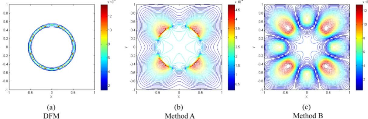
Fig. 5 shows that the main error in the computations are originated from the interface. This demonstrates the importance of using higher-order method

Figure 5: Contour of numerical error

Methods DFM Method A Method B

kEnk∞ Order kEnk∞ Order kEnk∞ Order

30 × 30 0.031 2.204e-3 6.867e-4

60 × 60 0.015 0.99 2.873e-4 2.94 1.072e-4 2.68

120 × 120 0.008 0.96 5.312e-5 2.43 3.286e-5 1.70

240 × 240 0.004 0.93 1.225e-5 2.16 8.134e-6 2.01

Table 3: Comparison of numerical errors

Example 4.2 In this example, we consider the discontinuous Poisson prob-lem with the elliptic interface:

Γ : x

2

a2 +

y2

b2 = 1,

and we use the notations

4u± = f± in Ω±,

[u] = w(s) on Γ, (77)

[un] = v(s) on Γ,

u = u0 on ∂Ω.

We derive the jump conditions [u] and [βun] from the exact solution. Four

different examples as shown in Table 4 are tested. Unlike in Example 4.1, the solution in this example is discontinuous.

Remember that in order to calculate the jump conditions (61) and (62),

we need the unit normal vector n = (n1, n2). In this example, we use

Case 1 Case 2 Case 3 Case 4

u− 1 x2− y2 excos(y) sin(x) cos(y)

u+ 1 + log(2

p

x2_{+ y}2_{) 0 0 0}

f− 0 0 0 −2 sin(x) cos(y)

f+ 0 0 0 0

Table 4: Four test cases for Eq. (77).

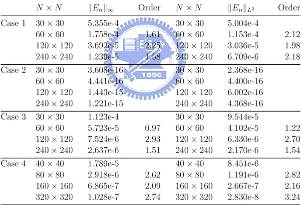
In Case 2, since the exact solution is a polynomial, the maximum errors are machine errors. Note that for Case 4, we use the different grids since the Cartesian grid cannot fetch the interface behavior if we use the same grid for other cases.

N × N kEnk∞ Order N × N kEnkL2 Order

Case 1 30 × 30 5.355e-4 30 × 30 5.004e-4

60 × 60 1.758e-4 1.61 60 × 60 1.153e-4 2.12

120 × 120 3.692e-5 2.25 120 × 120 3.036e-5 1.98

240 × 240 1.239e-5 1.58 240 × 240 6.709e-6 2.18

Case 2 30 × 30 3.608e-16 30 × 30 2.368e-16

60 × 60 4.441e-16 60 × 60 4.400e-16

120 × 120 1.443e-15 120 × 120 6.002e-16

240 × 240 1.221e-15 240 × 240 4.368e-16

Case 3 30 × 30 1.123e-4 30 × 30 9.544e-5

60 × 60 5.723e-5 0.97 60 × 60 4.102e-5 1.22

120 × 120 7.524e-6 2.93 120 × 120 6.330e-6 2.70

240 × 240 2.637e-6 1.51 240 × 240 2.170e-6 1.54

Case 4 40 × 40 1.789e-5 40 × 40 8.451e-6

80 × 80 2.918e-6 2.62 80 × 80 1.191e-6 2.82

160 × 160 6.865e-7 2.09 160 × 160 2.667e-7 2.16

320 × 320 1.028e-7 2.74 320 × 320 2.830e-8 3.24

Table 5: Comparison of numerical errors by method A with result for a = 0.6, b = 0.4.

4.3.2 Elliptic Equation

Example 4.3 We use the example, which was used by Leveque and Li[3] to test IIM in this thesis. An elliptic equation with a delta function source term and with a discontinuous coefficient β as follows:

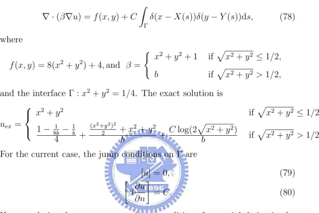
∇ · (β∇u) = f (x, y) + C Z Γ δ(x − X(s))δ(y − Y (s))ds, (78) where f (x, y) = 8(x2_{+ y}2_{) + 4, and β =} ( x2_{+ y}2_{+ 1 if} p_x2_{+ y}2 _{≤ 1/2,} b if px2_{+ y}2 _{> 1/2,}

and the interface Γ : x2_{+ y}2 _{= 1/4. The exact solution is}

uex =    x2_{+ y}2 _if p_x2_{+ y}2 _{≤ 1/2,} 1 − 1 8b − 1b 4 + (x2_+y2₎2 2 + x2+ y2 b + C log(2px2_{+ y}2₎ b if p x2_{+ y}2 _{> 1/2.}

For the current case, the jump conditions on Γ are

[u] = 0, (79) · β∂u ∂n ¸ = C. (80)

Here we derive the necessary two jump conditions for partial derivative by the method in Sec. 4.2.

C = 0.1 40 × 40 80 × 80 160 × 160 320 × 320

b kEnk∞ kEnk∞ Order kEnk∞ Order kEnk∞ Order

10.0 8.15e-5 2.53e-5 1.69 5.76e-6 2.14 1.38e-6 2.06

5.0 1.58e-4 4.97e-5 1.67 1.12e-5 2.15 2.71e-6 2.06

1.0 6.99e-4 2.31e-4 1.59 5.04e-5 2.20 1.24e-5 2.02

0.01 0.05985 0.02128 1.49 0.00431 2.30 0.00112 1.94

0.005 0.11961 0.04255 1.49 0.00861 2.30 0.00225 1.94

Table 6: Comparison of numerical errors

According to the exact solution, as b decreases, the maximum magnitude of |u(x, y)| increases. Therefore, the computational errors will increase when the value of b decreases.

Example 4.4 In this example, we consider the discontinuous elliptic equa-tion with elliptic interface:

Γ : x2

a2 +

y2

b2 = 1

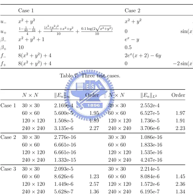
Case 1 Case 2 Case 3

u− x2+ y2 x2+ y2 x2− y2 u+ 1− 1 80− 1 10 4 + (x2+y2)2 2 +x2+y2 10 + 0.1 log(2√x2_+y2₎ 10 0 sin(x) cos(y) β− x2+ y2+ 1 ex− y 1 β+ 10 0.5 2 f− 8(x2+ y2) + 4 2ex(x + 2) − 6y 0 f+ 8(x2+ y2) + 4 0 −2 sin(x) cos(y)

Table 7: Three test cases.

N × N kEnk∞ Order N × N kEnkL2 Order

Case 1 30 × 30 2.169e-4 30 × 30 2.552e-4

60 × 60 5.600e-5 1.95 60 × 60 6.527e-5 1.97

120 × 120 1.508e-5 1.89 120 × 120 1.736e-5 1.91

240 × 240 3.135e-6 2.27 240 × 240 3.706e-6 2.23

Case 2 30 × 30 2.776e-16 30 × 30 1.086e-16

60 × 60 6.661e-16 60 × 60 1.833e-16

120 × 120 6.661e-16 120 × 120 1.535e-16

240 × 240 1.332e-15 240 × 240 4.247e-16

Case 3 30 × 30 2.093e-5 30 × 30 2.214e-5

60 × 60 8.626e-6 1.23 60 × 60 8.084e-6 1.45

120 × 120 1.449e-6 2.57 120 × 120 1.572e-6 2.36

240 × 240 5.628e-7 1.36 240 × 240 6.195e-7 1.34

Table 8: Comparison of numerical errors by method A with result for a = 0.8, b = 0.2.

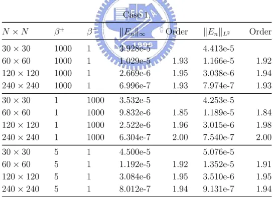
4.3.3 Application of Heat Equation

Example 4.5 We use the example used by Shen and Li[6], the heat equa-tion with an interface as follows

ut = ∇ · (β∇u), Ω = [−1, 1] × [−1, 1], t ∈ [0, ∞] (81) where β(x, y) = ( β− _{if (x, y) ∈ Ω}−_, β+ _{if (x, y) ∈ Ω}+_. (82)

We give the initial condition

u(x, y, 1) = exp µ −x 2_{+ y}2 4β ¶

and the Dirichlet boundary condition when (x, y) ∈ ∂Ω and two natural jump

conditions [u] and [βun] by the exact solution:

u(x, y, t) = 1 t exp µ −x2+ y2 4βt ¶ . (83) We use the Crank-Nicolson method in this example. The steps of our algo-rithm can be outlined as follows:

Step 1. Reinitialize φ to be an exact signed distance function by solving the

equation, φt = sgn(φ0)(1 − |∇φ|) to steady state.

Step 2. Compute outward normal vector n by Eq. (8). We compute this value

at grid points neighboring the interface, then we interpolate its value on the interface whenever it is needed. Eq. (8) is numerically solved using center difference approximations to the partial derivatives of φ.

Step 3. Use φ to determine a flag matrix F . For example, let F (i, j) = 0 if (xi, yj) is regular point;

F (i, j) = 1 if (xi, yj) is irregular point.

Then we can use F to determine what kind the grid points are. Also,

we compute the distance form irregular (xi, yj) to the interface in either

Step 4. Use the Crank-Nicolson method as following: un+1 i,j − uni,j 4t = 1 2(βi,j4u n+1

i,j + βi,j4uni,j).

Rearrange the equation above, we have

4t(βi,j4un+1i,j ) − 2un+1i,j = −4t(βi,j4uni,j) − 2uni,j (84)

Use F to distinguish grid points. For regular point, we use five-point

Laplacian to discretize 4un+1_i,j on the left hand side of Eq. (84). For

irregular point, we discretize 4un+1

i,j term by IIM in this thesis. This

scheme is always numerically stable and convergent but usually more numerically intensive as it requires solving a linear system AU = b of numerical equations on each time step.

Step 5. Since our interface is fixed, the matrix A is fixed. We repeat Step 4 to

get the solution u at next time step. Case 1. N × N β+ _β− _kE nk∞ Order kEnkL2 Order 30 × 30 1000 1 3.928e-5 4.413e-5 60 × 60 1000 1 1.029e-5 1.93 1.166e-5 1.92 120 × 120 1000 1 2.669e-6 1.95 3.038e-6 1.94 240 × 240 1000 1 6.996e-7 1.93 7.974e-7 1.93 30 × 30 1 1000 3.532e-5 4.253e-5 60 × 60 1 1000 9.832e-6 1.85 1.189e-5 1.84 120 × 120 1 1000 2.522e-6 1.96 3.015e-6 1.98 240 × 240 1 1000 6.304e-7 2.00 7.540e-7 2.00 30 × 30 5 1 4.500e-5 5.076e-5 60 × 60 5 1 1.192e-5 1.92 1.352e-5 1.91 120 × 120 5 1 3.084e-6 1.95 3.510e-6 1.95 240 × 240 5 1 8.012e-7 1.94 9.131e-7 1.94

Case 2. N × N β+ _β− _kE nk∞ Order kEnkL2 Order 30 × 30 1000 1 5.220e-5 4.855e-5 60 × 60 1000 1 1.352e-5 1.95 1.287e-5 1.92 120 × 120 1000 1 3.478e-6 1.96 3.336e-6 1.95 240 × 240 1000 1 8.674e-7 2.00 8.280e-7 2.01 30 × 30 1 1000 5.023e-5 5.092e-5 60 × 60 1 1000 1.363e-5 1.88 1.363e-5 1.90 120 × 120 1 1000 3.492e-6 1.88 3.439e-6 1.99 240 × 240 1 1000 8.963e-7 1.96 8.834e-7 1.96 30 × 30 5 1 5.884e-5 5.544e-5 60 × 60 5 1 1.537e-5 1.94 1.475e-5 1.91 120 × 120 5 1 3.947e-6 1.96 3.806e-6 1.95 240 × 240 5 1 9.903e-7 1.99 9.528e-7 2.00

Table 10: Numerical results with Γ : ¡ x

0.8

¢₂

+¡_0.2y ¢2 = 1, ∆t = h, T = 2.

5

Conclusion

The advantage of the IIM in this thesis is that the finite difference formulas at irregular points are expressed in an explicit form, so they can be applied to difference problems without modifications. But there are still hard work

when we use the natural jump condition [βun], so our method will fail if the

problem with concave interface.

Our future work is to calculate [un] by the relation

[un] =

[βun] − [β]u−n

β+ .

Thus, we have to solve the unknown term u−

n. Li[4] offered the method by a

similar method introduced in original IIM.

There are two challenges. First one is modify our IIM by the method introduced above. Second one is use the modified IIM to solve the Stefan problems[11, 12, 13].

Acknowledgments The method and most notations we used in this thesis are referred by Zhong[1]. Especially we thank Tsai for providing the code of re-initialization process.

References

[1] X. Zhong. (2007). A new high-order immersed interface method for solv-ing elliptic equations with imbedded interface of discontinuity, Journal of Computational Physis. 225, 1066-1099.

[2] Z. Li, K. Ito. (2006). The Immersed Interface Method : Numerical So-lutions of PDEs Involving Interfaces and Irregular Domains, SIAM. [3] R.J. LeVeque. (1994). Z. Li, The immersed interface method for elliptic

equations with discontinuous coefficients and singular sources, SIAM J. Numer. Anal. 31, 1001-1025.

[4] Z. Li. (1998). A Fast Iterative Algorithm for Elliptic Interface Problems, Journal on Numerical Analysis. 35, 230-254.

[5] Z. Li. (1997). Immersed interface methods for moving interface problems, Numerical Algorithms. 14, 269-293.

[6] Y. Shen, Z. Li, A numerical method for solving heat equations involving interfaces, Electron. J. Diff. Eqns., Conf. 03 (1999) 100-108.

[7] Y.C. Zhou, S. Zhao, M. Feig, G.W. Wei. (2006). High order matched interface and boundary method for elliptic equations with discontinuous coefficients and singular sources, J. Comput. Phys. 213, 1-30.

[8] A. Wiegmann, Kenneth P. Bube. (2000). The Explicit-Jump Immersed Interface Method: Finite Difference Methods for PDES with Piecewise Smooth Solutions, SIAM , Journal on Numerical Analysis, 37, 827-862. [9] A. Mayo. (1984). The fast solution of Poissons and biharmonic equations

on irregular regions, SIAM J. Numer. Anal. 21, 285-299.

[10] S. Osher, R. Fedkiw. (2003). Level Set Methods and Dynamic Implicit Surfaces, Springer.

[11] S. Chen, B. Merriman, S. Osher and P. Smereka. (1997). A simple level set method for solving Stefan problems, Journal of Computational Ph-ysis. 135, 8-29.

[12] Z. Li. (1997). Immersed interface methods for moving interface problems, Numerical Algorithms. 14, 269-293.

[13] Z. Li, B. Soni. (1999). Fast and accurate numerical approaches for stefan problems and crystal growth, Numerical Heat Transfer, Part B, 35,