有效率的方塊式繞線器使用繞線圖形簡化法

國

立

交

通

大

學

資訊科學與工程研究所

碩

士

論

文

有效率的方塊式繞線器使用繞線圖形簡化

法

An Efficient Tile-Based Router with Routing Graph

Reduction

研 究 生：陳文彬

指導教授：李毅郎 博士

有效率的方塊式繞線器使用繞線圖形簡化法

An Efficient Tile-Based Router with Routing Graph Reduction

研 究 生：陳文彬 Student：Wen-Bin Chen

指導教授：李毅郎 Advisor：Dr. Yih-Lang Li

國 立 交 通 大 學

資 訊 科 學 與 工 程 研 究 所

碩 士 論 文

A Thesis

Submitted to Institute of Computer Science and Engineering College of Computer Science

National Chiao Tung University in partial Fulfillment of the Requirements

for the Degree of Master

in

Computer and Science

Oct 2005

Hsinchu, Taiwan, Republic of China

有效率的方塊式繞線器使用繞線圖形簡化法

學生：陳文彬 指導教授：李毅郎 博士

國立交通大學 資訊科學與工程研究所 碩士班

摘 要

當製程技術進展到奈米科技的時代，電路信號的延遲和雜訊的最佳化是整個積體電路 設計中最關鍵的一環。這些最佳化的問題可以由改變導線尺寸和加大導線的間距來達到。與 網格式繞線器相較，方塊式繞線器能夠更有效率的處理導線線寬及線距的問題。為此，這篇 論文中我們針對整個晶片的繞線問題建置了一個有效率的方塊式繞線器。另外，我們亦將繞 線圖形的簡化法整合到兩階段式的繞線流程之中。第一階段是一個通用的全域繞線器， 此全域繞線評估整個晶片繞線資源的分佈情形來決定全域路徑。而此全域路徑導引第二 階段的細部繞線器來決定在佈局上的實際路徑。繞線圖形簡化法移除冗贅的方塊及切齊 相鄰方塊來減少佈局中方塊碎裂的情形，進而提高了方塊式繞線器的執行效率而且不會 因簡化繞線圖形而犧牲繞線品質。此外我們還提出一個區段樹的資料結構來儲存多重端 點的接線，此資料結構可以幫助我們更有效率地去處理拔除重繞的程序。實驗結果顯 示，我們的方塊式繞線器跟多重層次架構的繞線器比較起來能夠更迅速的完成繞線並且 獲得更好的繞線結果。

An Efficient Tile-Based Router with Routing Graph Reduction Student: Wen-Bin Chen Advisor：Dr. Yih-Lang Li

Institute of Computer Science and Engineering National Chiao Tung University

ABSTRACT

As technology advances into the nanometer era, the interconnect optimization for the delay and noise issues is the dominant factor to the modern IC design. These optimizations impose the wire sizing and spacing to the interconnections .Gridless router is more applicable to handle the various design rules than grid router. Therefore, we develop an efficient tile-based router for the full chip routing in this thesis. This work integrates the routing graph

reduction into the two-stage routing flow. The first stage is a general global router, which

estimates the routing resource to decide a rough path for the detailed router. According to the result of global routing, the tile-based router, the second stage, completes the full chip routing net by net. Routing graph reduction involves the removal of redundant tiles and alignment of neighboring tiles to reduce the fragment of the tile plane and accelerate the routing speed of tile-based router. We also propose a segment tree to help the rip-up and reroute procedure work more flexibly and efficiently. Segment tree maintains the Steiner tree of multi-terminal net segment by segment so that the rip-up and reroute procedure just rip-up and reroute the violated segment instead of the entire net. Experiment results show the expeditious routing speed and better routing solution than multilevel framework.

Acknowledgements

I am deeply grateful to my advisor, Dr. Yih-Lang Li for his continuous guidance, support, and ardent discussion throughout this research. His valuable suggestions help me to complete the thesis. Also I express my sincere appreciation to all classmates in my laboratory for their encouragement and help.

This thesis is dedicated to my parents and my families for their patience, love, encouragement, and long expectation.

Contents

Abstract (in Chinese)... I Abstract (in English)... II Acknowledgements...III List of Figures ...V List of Tables...VI

1 Introduction ... 1

1.1 Gridless Router... 2

1.2 Routing Graph Reduction…... 5

2 Preliminaries………... 7

2.1 Tile-Based Router... 7

2.2 Routing Dabase………. 9

3 Routing Flow………... 11

3.1 General-Puropose Routing with Routing Graph Reduction... 13

3.2 Rip-up and Reroute ………... 17

4 Segment Tree……... 19 4.1 Data Structure………... 19 4.2 Tree Operation………... 21

4.2.1 Node Insertion... 21 4.2.2 Node Deletion………...26 4.2.3 P-node Feting………31 5 Experimental Results... 32 6 Conclusions... 36 Bibliography... 37

List of Figures

1.1 Routing models... 3

1.2 Tile-based graph... 4

1.3 Routing graph reduction... 6

2.1 Contour example... 8

2.2 Tile propagation... 9

2.3 Quadtree example... 10

3.1 The flowchart of routing ... 12

3.2 The space tile density example... 14

3.3 Recycling the redundant tile... 16

3.4 The rip-up and reroute algorithm…... 18

4.1 An example of S-tree... 20

4.2 Node insertion case(1)... 22

4.3 Node insertion case(2) ... 23

4.4 An incomplete net and S-tree... 24

4.5 Node insertion case(3) ... 25

4.6 Node deletion case(1)... 27

4.7 The net of node deletion case(2)... 29

4.8 The splitting process of node deletion case(2)... 30

List of Tables

2.1 Object assignment rule... 10

5.1 The benchmark circuits... 32

5.2 Routing results comparison... 33

5.3 Apply Redundant Tiles Removal………. 34

Chapter 1

Introduction

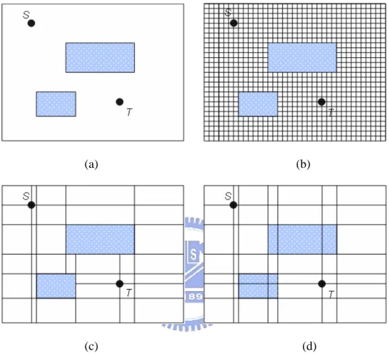
The current IC design trend is toward integrating system on a chip (SoC). Such a SoC solution is highly complicated and time-consuming. Time-to-market pressure forces IC design houses have to reuse intellectual properties (IP) to fabricate a new chip. But these IPs may be designed with the different width and spacing individually. Therefore, the interconnection of the variable wire width and variable spacing between these IPs becomes the critical issue of the design. However, the traditional grid router is not suitable for routing the complex SoC design. Because the different design rules evolve the greatly dense grids that would induce the large amount of memory space and searching time,as shown in Figure 1-1 (b). The advantage of gridless router is that it deals with the wire width and spacing rules and makes routing in the SoC design more efficient.

1.1 Gridless Router

There are two approaches of gridless routers [5-15]. One uses the connection graph-based algorithms [5]. This approach according to the design rules expands the boundaries of each obstacle with a specific size then reaches out these extended lines until touching the expanded boundaries of other obstacles or borders of the routing region. The intersecting points form the nodes of the routing graph, as shown in Figure 1-1(c). However this connection graph is hard to build and update for incremental routing all nets. Cong et al [6-8] proposed an implicit connection graph in which every node is the intersecting point of all extended boundaries of the obstacles. Actually, searching path at some nodes might cause the design rule violation; hence they using a fast query data structure to get the available node of routing graph, Figure 1-1(d) displays a routing graph of this model. Obviously, the number of generated nodes is more than Zheng[5] in spite of Cong also showed the efficiency of the graph creation and the optimality of the routing path. The question is when a great number of nodes arisen from the large design, the connection graph models bring about the inefficient path search.

(a) (b)

(c) (d)

Figure 1-1: Routing models. (a) Two terminals and obstacles; (b) grid model; (c) connection graph model; (d) implicit connection graph model.

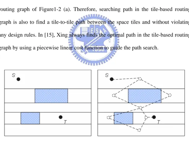
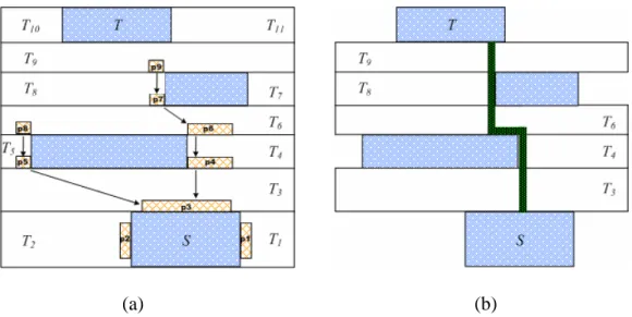
Another approach is the tile-based model [9-15], which represents the routing region based on the corner-stitching data structure [16]. Corner-Stitching represents the obstacles existed in the routing region as block tiles while the free areas are related to space tiles. Every tile contains four corner pointers to stitch four adjacent tiles and keep the property of maximum horizontal (vertical) strip. Base on this structure, it provides some fast and localized operations, such as neighbor searching and region querying, which will benefit searching a path in the routing graph. Figure 1-2 (a) depicts a tile pane with the maximum horizontal strips. Every space tile in the tile plane corresponds to a node in the routing graph, and every edge between two nodes indicates the adjacent relation of tiles, Figure 1-2 (b) represents the corresponding routing graph of Figure1-2 (a). Therefore, searching path in the tile-based routing graph is also to find a tile-to-tile path between the space tiles and without violating any design rules. In [15], Xing always finds the optimal path in the tile-based routing graph by using a piecewise linear cost function to guide the path search.

(a) (b)

Figure 1-2. (a) A tile plane with maximum horizontal strip; (b) the corresponding routing graph.

1.2 Routing Graph Reduction

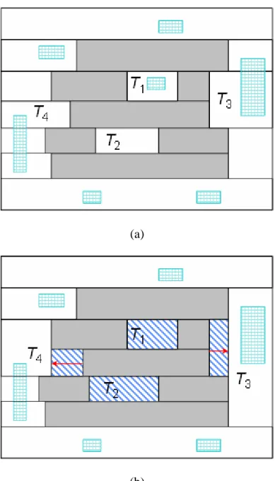
For several hundred millions gates design, a great quantity of routing paths will come into existence when the routing process begins. The existed paths increase not only the fragmentation of the plane but also the complexity of the path search. Li [23] introduced two methods of the routing graph reduction (RGR) to reduce the fragmentation and accelerate the routing speed. One is the removal of redundant tiles; another is the alignment of the neighboring tiles.

Redundant tiles removal, which removes one-conjunct tiles and 0-conjunct tiles in the tile planes by using the operation of tile enumeration. While alignment of neighboring tiles shrinks the ragged boundaries and merges shrunk tiles to reduce the fragmentation. Figure 1-3 (a) shows an original tile plane. In Figure 1-3 (a), T1 is a

one-conjunct tile while T2 is a 0-conjunct tile. Figure 1-3 (b) displays the final result

of routing graph reduction. T3 and T4 are aligned merged with neighbor tiles.

The purpose of this thesis is to integrate RGR algorithm into the two-stage routing flow and improve the routing speed. Additionally, we propose a novel data structure to handle the rip-up and reroute more flexibly and efficiently. The rest of this thesis is organized as follows. Chapter 2 briefly reviews the point-to-pointer routing engine and the routing database. Chapter 3 describes the two-stage routing flow and how to apply RGR algorithm. Chapter 4 presents the segment tree structure. The experimental results are shown in Chapter 5. Finally, Chapter 6 draws the conclusions.

(a)

(b)

Chapter 2

Preliminaries

2.1 Tile-Based Router

Since Ousterhoust [16] proposed the corner stitching for representing and manipulating rectilinear layout, there have many studies on the tile-based router [9-15] to find the tile-to-tile path. In [14] introduced the concept of contour, where the tile-based router search the centerline path within the contour planes which is constructed by extending the already existed shapes in the tile plane with size ws +

ww/2 – 1/2, where ws is the spacing rule for the net to be routed to the related layer, ww

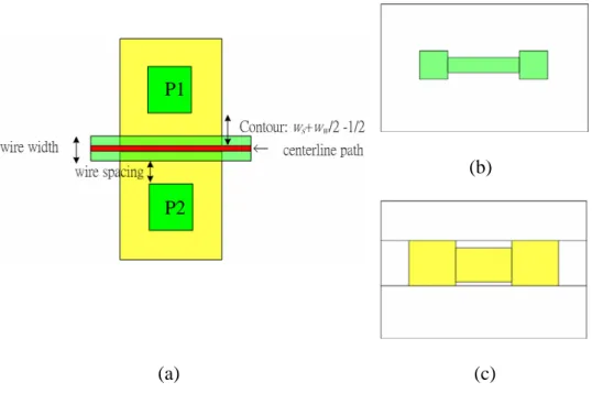
is the wire width. The contour planes could guarantee that any path routed on the space tiles would not induce the design violations. For example, in Figure 2-1 the two yellow blocks are the contour induced from P1 and P2. If the space between two blocks allows a centerline path passed. After extending the centerline path with the wire width, the new path would separate away from P1 and P2 with the wire spacing. Figure 2-1(c) shows an example for represent the contour plane of Figure 2-1(b).

P2 P1

(b)

(a) (c)

Figure 2-1. A contour example. (a) The contour size; (b) metal layer; (c) the related contour plane of (b).

Tile-based router for full chip routing consists of three stages – path entry initialization, tile propagation and path construction. Path entry initialization places the zero cost entry segments into the tiles that abut the source blockages. For example, in Figure 2-2(a), the entry segments p1, p2 and p3 are placed in the T1, T2 and T3, respectively. In the tile propagation stage, the entry segment with the pre-defined cost is propagated to the neighboring space tile in the current layer or the adjacent layer that allows a via to connect the space tiles in the different layer. A path entry segment will be created in the next tile if the propagation from the current tile could generate the minimal-cost path to it. The backward pointer of entry segment points to the previous tile that propagates to it. The entry segment p3 in Fig. 2-2(a) is propagated to tile T4 then induced an entry segment p4 whose backward pointer points to p3. If the target is found, the list of free tiles is derived from the backward pointer. Finally, the path constructor produces the minimum-corner path in the list of free tiles. Figure 2-2(b) indicates the new path over the tile list T3, T4, T6, T8 and T9.

(a) (b)

Figure 2-2. (a) The tile propagation example; (b) path construction.

2.2 Routing Database

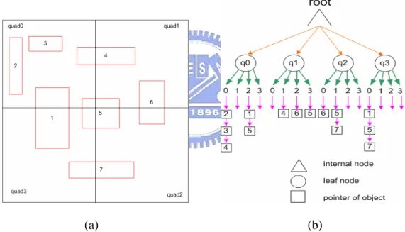
During our routing process, both segment tree and rip-up overlapped tiles need an efficient data structure that can provide a fast region query operation. The operation of region query is a request to find all objects that intersected with a specified query area. There were many studies on this topic [17-20]. In our router, we adopt the method of Weyten and Pauw [20]. They proposed a quad-list quad tree (QLQT) structure to store geometrical data. In QLQT, every node represents a quadrant region in the plane. Each quadrant may be subdivided into four sub-quads when total number of objects it contained more than a threshold value. If the rectangular object intersects with a leaf node, a pointer of the rectangular object will be stored in the one of quad-list of the leaf node. The rules used to assign pointer to list are shown in Table 2-1. According to the result of checking rules, the pointer is assigned to where it should be stored. Figure 2-3 is an example shown how the objects are stored in the list of the leaf nodes. In Figure 2-3(a) rectangle 2 and 3 don't cross any boundary of q0; therefore, they are stored in the list-0 of q0. Rectangle 6 crosses the lower boundary of q1; hence, the pointer of rectangle 6 will be saved in the list-2

of q1 and the list-1 of q2. Now, consider the case of rectangle 5. Because it intersects with four quadrants, so we will keep the pointer of rectangle 5 in each quadrant.

Table 2-1. Object assignment rule. object’s lower boundary

crosses leaf’s lower boundary.

object’s left boundary crosses leaf’s left boundary

list type False False 0 False True 1 True False 2 True True 3 (a) (b)

Figure 2-3: An example shows how the objects are stored in the list of the leaf nodes.

Chapter 3

Routing Flow

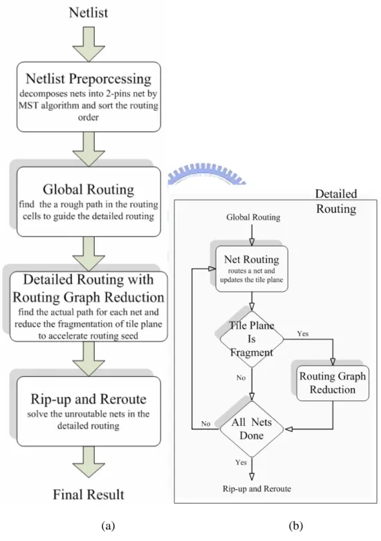
Figure 3-1(a) presents the routing flow of out tile-based router. In the preprocessing stage, the minimum spanning tree (MST) algorithm is applied to decompose every multi-terminal nets ni into a set of two-terminal nets {ni1, ni2, …,

nim}. The routing order of all the two-terminal nets is also determined in this stage.

The routing order is in an increasing order of the Manhattan distance of each two-terminal net. Global routing follows the net preprocessing to obtain a global path for each two-terminal net. The routing region is first partitioned into several global cells, and global router searches for a global path of minimum length for each net under the global cell congestion constrain. Although each multi-terminal net is partitioned into several two-terminal nets using minimum spanning tree algorithm, the global routing path of a net is a Steiner-tree by performing a point-to-path (path-to-path) global routing if one (both) of the terminals of current point-to-point routing has (have) been included in a complete global routing path.

To collaborate with global routing, the kernel of the tile-based router is not merely a point-to-point router. Extended routings, such as point-to-component (P2C) and component-to-component (C2C) routings are supported in the routing kernel. Segment-tree (S-tree) also provides fast component fetching operation for the preprocessing tasks of P2C and C2C routings. Section 4 will formally present S-tree. When a net routing is completed, the found routing path is added to the corner-stitching tile planes and the S-tree of that net. After performing some net routings, the tile fragmentation of the corner-stitching tile planes are examined and the

routing graph reduction (RGR) method will be applied to diminish the tile fragmentation if the tile planes are over-fragmented. Figure 3-1(a) displays the entire routing flow, while Fig. 3-1(b) shows the detailed routing flow including routing graph reduction. Rip-up and reroute operation aims at solving all routing violation using dirty routing, which will be discussed in more details in Section 3-2.

(a) (b)

3.1 General-Purpose Routing with Routing Graph Reduction

Li [23] proposed a novel routing graph reduction method to diminish tile fragmentation and to improve the performance of ECO tile-based routing. In this thesis, the redundant tiles removal is applied to general-purpose tile-based router.

The main concept of the work is to perform redundant tiles removal when the routing tile planes are over-congested; therefore, the scheme to measure the exact degree of tile fragmentation is indispensable for efficient tile plane check and simplification. Frequent redundant tile removal operation can not contribute to great improvement in routing performance; instead, the penalty of redundant tile removal operations getcauses Consequently, it is necessary to know in what kind of the situation we should apply the defragment procedure. In this section, we use an estimating mechanism to involve the defragment procedure.

To apply defragment procedure at the proper timing, we maintain the information of density of the space tiles during the process of routing. The density value SD shows

how fragment the tile plane is. The higher this value, the more fragment of the routing region is. We would involve the defragment procedure to reduce the fragmentation of layout if SD greater than a threshold value. SD is calculated by the following equation.

n SC SD n i i/ 1

∑

= =

Where SC is the count of space tiles in each panel, n is the total number of panels.

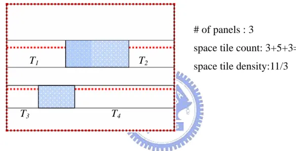
It is very easy to get the space tile count in each panel using the area enumeration algorithm of corner-stitching to visit the specific panel. Although this enumeration algorithm will count some tiles doubly, but in the larger design this small miscalculation could be ignored. In the beginning of the detailed routing, each routing layer is divided into several panels in their prefer direction. The advantage of dividing

panel in prefer direction is that the new routing path would induce or merge space tile in prefer direction too. Therefore, we could update the count information of the panel locally and calculate a new SD quickly. Every time routing a net is completed, only

routing path passed panels would need to recount the space tiles. Figure 3-2 is an example to indicate how to calculate SD. In Figure 3-2, T1, T2, T3 and T4 would be

counted twice, so the total count of space tile is 11 and the density value is 11/3.

T

4

T

3

T

2

T

1

# of panels : 3

space tile count: 3+5+3=11

space tile density:11/3

Figure 3-2. An example illustrates the space tile density.

If all panels have been updated we choose the current SD as the base density BD,

and check the criterion to apply defragment procedure to reduce tiles. The criterion is defined as,

SD > BD * AR

Where AR is the applying ratio, we can adjust AR to control the number of times of the defragment procedure. Nevertheless, it is possible after defragment procedure finished while the criterion still holds. It means, in the next time, when routing net completed we would apply the procedure again. For this season, we will increase AR with a small value when SD is not reduced too much.

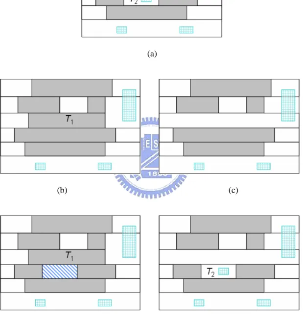
The defragment procedure using another tile color to represent the redundant tiles instead of considering as the block tiles. It is easy to get along with rip-up and reroute procedure. Because we might rip up some nets to release the routing resource in the rip-up and reroute procedure, if we treat the redundant tile in different color, then it will be easy to check whether the redundant tile should be recycled. In the Figure 3-3 (a) T2 is a redundant tile. If we consider T2 as a block tile as shown in

Figure 3-3 (b), T2 would be merged with neighbor tiles. When T1 is ripped, as shown

in Figure 3-3 (c), a path through T2 to adjacent layer disappeared too. Figure 3-3(d)

depicts that T2 is represented straightly. Figure 3-3(e) shows the result with a possible

(a) (b) (c) (d) (e)

3.2 Rip-up and Reroute

In the complex design, usually, the detailed router is very difficult to connect all

nets straightly. Therefore, it is necessary to perform the rip-up and reroute procedure

to complete the routing. This phase allows dirty routing which routes uncompleted net

overlapped with different signal nets. The dirty routing propagates both space and

block tiles to find a dirty path in the contour planes. A dirty path is the path of a net

with minimum of design rule violations to other nets. But the contour plane does not

keep any net information in the tiles. We query quad-tree to know which segments

overlapping with this dirty path. We would rather rip-up and reroute the overlapped

segment than the entire net. If it can’t find out the path then marks the net as

un-routable and perform dirty routing in the next iteration of rip-up and reroute.

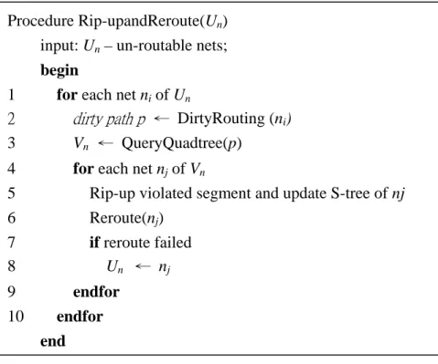
Figure 3-4 presents the algorithm of rip-up and reroute. Where Un is the set of

Procedure Rip-upandReroute(Un)

input: Un – un-routable nets;

begin

1 for each net ni of Un

2 dirty path p ← DirtyRouting (n_i)

3 Vn ← QueryQuadtree(p)

4 for each net nj of Vn

5 Rip-up violated segment and update S-tree of nj 6 Reroute(nj) 7 if reroute failed 8 Un ← nj 9 endfor 10 endfor end

Chapter 4

Segment Tree

Rip-up and reroute is a time-consuming stage during detailed routing, so a powerful and flexible scheme for rip-up and reroute can fast resolve the un-routable errors or design rule violations. In this section, we introduce a novel tree structure, called segment tree (S-tree), for efficient rip-up and reroute on the tile-based routing.

A general single net routing problem is to connect a set of terminals, T= {t1, t2, …,

tn }, with a set of wire segments, W= { W1, W2, …, Wm}, which are composed of the

shapes of the metal and via layers. The S-tree is a rooted tree, which contains two kinds of nodes, called Steiner nodes (s-node) and path nodes (p-node). An s-node is either a Steiner point or a net terminal and can be used to reserve the global topology of a net, while a p-node can be a wire or a via segment.

4.1 Data Structure

Segment tree is used to represent the routing paths of a net. One net terminal is the root s-node of a segment tree and the others are the leaf s-nodes. Each s-node, except the root node, has a forward pointer pointing to another s-node closer to root s-node. In Fig. 4-1, there are three net terminals and one Steiner point. The leaf s-nodes are terminals A and B and their outward edges point to the s-node of the Steiner point, whose related s-node finally points to the root s-node, that is, terminal C. Segment tree only describes the global topology of a routing path. Physical wire and via segments must be embedded in the segment tree. Since the edge of an s-node stands for a routing path from one point to another, a physical pointer is attached to each

s-node to indicate the start path segment of the routing path that realizes the forward edge. The path segments along the routing path are then linked by their internal pointer and the last segment can point to null to show the end of a path. Each s-node also contains a number to identify its type, where a net terminal s-node has a net terminal number and a Steiner point s-node has a number of zero.

(a) A three-terminal net and its connected path.

(b) The corresponding S-tree.

Figure 4-1: An example shows the structure of S-tree. A path node contains the following information:

z The x and y coordinates of the path segment’s bottom left and top right corners.

z The net field denotes the net number of the path segment and the layer field denotes the routing layer of the path segment.

z A path pointer, which points to the p-node of the following path segment to form a list. The last p-node is set to null.

z A topology pointer, which points back to the s-node.

For example, the routing path between terminal A and Steiner point S in Fig. 4-1 contains five path segments; five path segments can then be accessed from s-node SA

through its physical pointer.

4.2 Tree Operation

Three operations, node insertion, node deletion, and p-node fetching, for the query and manipulation of the S-tree will be presented in this sub-chapter. Based on these operations, the rip-up and reroute process could efficiently query net information. The time complexity of each operation will be also discussed to show the efficiency of the S-tree structure.

The following notation is first introduced before describing the above operations. z Fs(si): the preceding s-node of a s-node si.

z Tw(si): the last p-node of a path associated with the s-node si.

z Pw(pi): the path pointer of p-node pi.

z Ms(pi): the topology pointer of p-node pi.

4.2.1 Node Insertion

A multi-terminal net has been decomposed into several 2-terminal nets in the preprocessing stage. The tile-based detailed router routes 2-terminal net one by one in the routing order. When a net routing is completed and the new routing path is inserted to the corner-stitching tile planes, the S-tree has to be also updated to maintain the new tree structure. Three cases are considered for the operations of

saving a routing path and updating the S-tree.

Case (1): a new path connects a new terminal T1 to another terminal T2 with a set

of path segments, P= {P1, P2, …, Pm}, i.e., T1 can reach T2 by passing through the

sequence of the path segments from P1 to Pm. If terminal T2 has an associated s-node,

a new s-node is created for T1 and pointed to the s-node of T2. On the contrary, if

terminal T2 is also a new terminal, a new s-node is created for T2 and assigned as the

root of the new tree; besides, a new s-node sn1 is created for T1 and Fs(sn1) is set to be

T2. Figure 4-2 shows an example of Case (1), where terminal B connects to another

new terminal C through three path segments. A new s-node SC is created for terminal

C and assigned as the root of the S-tree and the forward pointer of the new s-node SB

of terminal B points to SC, as shown in Fig.4-2(b).

(a) (b)

Figure 4-2: An example for Case (1) of node insertion.

Case (2): a new routing path, which consists of a set of path segments, connects a new terminal to an existing path segment Pe with a set of path segment, P= {P1, P2, …,

Pm}. In this case, a Steiner point Sp will be produced at the join of Pm and Pe. Figure

4-3 (a) shows that the terminal A is connected to a path segment c1 in the routing path

connecting terminals B and C. The detailed process of updating the S-tree is explained in the following through Figs. 4-3 (b) to (e).

1) A query operation for the path segment c1 is first performed on the quad-tree to obtain the pointer of c1 and then the s-node to which c1 is attached through

2) Since a new Steiner point is produced on the path segment c1, a new s-node S1

must be created here to maintain the tree structure. Fs(S1) is set to be Sc and Tw(S1)

is set to be c2, as shown in Figure 4-3(b).

3) When a connection in the S-tree is divided into 2 parts and a new s-node is inserted, the routing path of the original connection also has to be divided into two parts which are attached two s-nodes. In Fig. 4-3(c), path segment c2, c1, and

b1 are divided into two parts and b1 is attached to the original s-node SB while c2

and c1 are attached to the new s-node S1. Also Tw(SB) is set to be b1, and Tw(S1) is

set to be c2.

4) Five new p-nodes are created for the new routing path, a1, a2, a3, a4, and a5.

They are all attached to the new s-node of terminal A, as shown in Fig. 4-3(d). 5) Finally, FS(SA) is set to be S1 to finish the construction of the new Steiner tree,

as shown in Fig. 4-3(e). Figure 4-3(f) illustrates the physical path segments associated with the S-tree in Fig. 4-3(e).

(a) (b)

(e) (f)

Figure 4-3: An example to show the updating sequence.

Case (3): During routing and the construction of the S-tree, more than one S-tree may simultaneously exist. Figure 4-4(a) depicts an incomplete net routing which contains two connected routing paths and Fig. 4-4(b) show its related S-trees. The complete net routing will merge these two routing paths, so the operation of merging two S-trees must be considered and provided.

(a) (b)

Figure 4-4. (a) One incomplete net with two connected components; (b) its corresponding S-tree.

Considering the case of using a routing path of a set path segments P= {P1,

P2, …, Pm} to connected these two routing paths on the path segments of Pi and Pj.

merging two S-trees. In Fig. 4-5(a), two disjoined components are connected by the path segments i1 and i2 and two Steiner points S2 and S3 are produced on two S-trees.

The first three steps of S-tree merging operation are the same as those in the case (2). 1) Figures 4-5(b) to (d) depict the process of the insertion of a Steiner point in the

S-tree and the division of the routing path containing the Steiner point.

2) Since the new Steiner point is connected to another S-tree through the new routing path segments i1 and i2, the new Steiner point must temporarily act as

the new root of this S-tree before merging. Figures 4-5(e) and (f) shows the pre-process of a new root insertion.

3) In order to reserve the forwarding property of the S-tree, a reversing tree operation is provided. Assume the new Steiner point SP is located between two

s-nodes, say S1 and S2, and S1 points to S2. SP connects to another S-tree to form

a new S-tree. The reverse tree operation is to modify the S-tree structure such that SP becomes the new root by reversing the forward pointers along the list

from S2 to the old root. Also the path segments attached to each s-node along

the list must be reversed. The sub-tree outlined by bold dotted line in Fig. 4-5(g) shows the reverse result. A final S-tree is obtained by pointing SP to the other

new Steiner point on another S-tree, as shown in Fig. 4-5(g).

(d) (e)

(f) (g)

Figure 4-5: The processes of case(3).

4.2.2 Node Deletion

During the rip-up and reroute stage, the dirty routing completes those un-routable nets by passing through existing path segments. The overlapped path segments then have to be ripped up for cleaning design rule violations. Because the contour planes have no information about the overlapped segments, a query on the quad-tree is performed to obtain the net and geometrical information of the overlapped segments. The ripped-up operation has to be applied to corner-stitching tile planes as well as the S-trees. The main objective of deletion operation on the S-tree is to preserve the forwarding property of the S-tree. Two cases are considered for the deletion operation.

To simplify the description, the following discussion is based on the assumption that the root s-node will only be pointed by one s-node; besides, the net routing will not produce the crossing pattern and the most complex pattern is the T pattern. As a matter of fact, this thesis has extended the capability of segment tree beyond the above limitation.

Case (1): The dirty path segment is attached to a leaf s-node SB. Two conditions

for different types of the s-node S1, to which the forward pointer of s-node SB points,

are discussed in the following. (I) If s-node S1 is the root, all p-nodes and two s-nodes

are freed and the S-tree is degenerated into two terminals. (II) If s-node S1, whose

forward pointer points to s-node SC, is not the root and another s-node SA also points

to s-node S1 through its forward pointer. After s-node SB is deleted, s-node S1 is not a

Steiner point any more and can be removed. Therefore, s-node SA can directly points

to s-node SC and the p-nodes, which originally are attached to s-nodes S1 and SA, must

be linked together. The physical pointer of s-node SA is set to be the physical pointer

of s-node S1 and the last p-node of s-node S1 points to the physical pointer of s-node

SA. Figure 4-6 shows the case, where path segment b1 will be ripped-up and the

routing path will become two disconnected components after removing b1, as shown

(a) (b)

(c) (d)

(e)

Figure 4-6. The process of updating S-tree by removing a leaf s-node. (a) b1 is a dirty

path segment; (b) the net routing is composed of one routing path and one disjoint terminal after removing b1; (c) the original S-tree; (d) s-node S1 becomes non-Steiner

and disappears; the p-nodes of SA and S1 are combined; (e) final result.

Case (2): The dirty path segment is attached to internal s-node S2 and the s-node

S1, to which the forward pointer of s-node S2 points, is also internal. After removing

all p-nodes attached to S2, the S-tree will be split into two sub-S-trees and s-nodes S1

and S2 will disappear. Figure 4-7 (b) shows an example of a net with a dirty segment.

1) S-node SB’s forward pointer also points to S1 and s-node S1’s forward pointer

points to SC. Since the Steiner point S1 disappears after removing s-node S2, s-node

SB must directly connect to SC. The physical pointer of SB is set to the physical

pointer of S1 and the last p-node of S1 connects to the first p-node of SB. The

process is shown in Fig. 4-8(b).

2) The sub-tree below S2 forms another S-tree and its root is the terminal s-node, say

SA, whose forward pointer points to S2.

3) If another internal s-node S3 also points to S2, the path segments in S3 and SA must

be linked together and S3 directly points to the new root SA. The sequence of the

p-nodes of the new root SA is reversed and the new last p-node connects to the first

p-node of S3 and the physical pointer of S3 is set to be the new first p-node, as

shown in Figs. 4-8(c) and (d).

Figure 4-7: An example of a net routing for node deletion Case (2). (a) a3 is a dirty

path segment and all the p-nodes in S2 will be removed; (b) the net routing are

composed of two connected components after ripping-up the path segments a3, a4, and

a5.

(a) (b) (c) (d)

Figure 4.8: The process of splitting a S-tree into two S-trees by removing an internal s-node (a) a3 is a dirty segment and all p-nodes of S2 are removed; (b) s-node S1

becomes non-Steiner and the p-nodes in S1 and SB are connected to form a new S-tree;

(c) the sub-S-tree below S2 forms another new S-tree by selecting terminal s-node SA

as the new root and linking all the p-nodes in S3 and SA together; (d) the final two

4.2.3 p-node Fetching

Both point-to-component and component-to-component routing require fetching the p-node of tree to initial the routing process. This operation is implemented by storing the pointers of all s-nodes of an S-tree in a linked list. Another memory-efficient method is to store the pointers of all leaf s-nodes of a tree in a linked list, the S-tree can traversed by starting traverse at each leaf s-node.

Chapter 5

Experimental Results

We implemented our tile-based router in this work using the C++ language on the 1.2GHz SUN Blade 2000 workstation with 2GB memory. We compare our tile-based router to multilevel framework [21,22] with six benchmark circuits provided by the authors. Table 5.1 indicates the information of these six circuits; include the circuit dimensions, design rules, number of routing layers, total of 2-terminal nets and the number of terminals.

Table 5.2 shows the comparisons on wire length, the number of via, run-time and the completion rate. The results show that our approach could achieve average 4.7X and 7.2X faster routing speed than [21] and [22]. The S-tree for multi-terminal routing also brings better wire length and number of via than others by about 3% to 10%.

Table 5.1. The benchmark circuits. Circuits

Name Size(μm) Design rules(μm) #Layers #2-terminal Nets # Terminals S5378 4330x2370 3.6 3 3124 4734 S9234 4020x2230 3.6 3 2774 4185 S13207 6590x3640 3.6 3 6995 10562 S15850 7040x3880 3.6 3 8321 12566 S38417 11430x6180 3.6 3 21035 32210 S38584 12940x6710 3.6 3 28177 42589

Table 5.2. Routing results comparison.

Circuits Enhanced multilevel routing with rip-up and reroute [21]

Multilevel Routing without antenna avoidance [22] Our results Name Wire length #Vias Runtime (sec.) Cmp. Rates Wire length #Vias Runtime (sec.) Cmp. Rates Wire length #Vias Runtime (sec.) Cmp. Rates

S5378 8.0e7 7197 34.3 99.74% 8.2e7 7163 35 100% 7.7e7 6410 5.27 100%

S9234 5.9e7 6155 24.4 99.89% 6.0e7 6287 26.2 100% 5.7e7 5461 3.53 100%

S13207 1.9.e8 15832 115.4 99.83% 2.2e8 14938 106.7 100% 1.8e8 14185 20.42 100% S15850 2.3.e8 18778 154.6 99.88% 2.4e8 17334 538.8 100% 2.2e8 16900 42.65 100% S38417 5.0e8 45620 567.6 99.80% 5.9e8 43551 899.9 100% 5.0e8 41376 111.59 100% S38584 7.0e8 63205 1308.2 99.84% 7.7e8 61053 1953.7 100% 6.9e8 56233 379.11 100%

Avg. 3.0% 10.5% 4.7X 10.5% 7.3% 7.2X

In Table 5.3, we compare the tile-based router with and without RTR at the

detailed routing stage. However, the results indicate that the routing time almost is not

improved, instead getting worse. It produced a contrary to our intention. It is

interesting to note that if the tile plane is more fragmented the redundant tiles removal

could produce the better reduction result. Besides, the time for determining the

over-fragmented tile planes and performing RTR would increase the total of runtime.

The reduced rate denoted in the final column of Table 5.3 shows that these six circuits

are too sparse to reduce the redundant tiles and speedup the routing process.

The operation time spent on S-tree and Quad-tree are list in Table 5.4. In the table, the second and fifth column indicates the time for updating S-tree and quad-tree that includes the insertion and deletion time. In third column, “Query” shows the time to fetch p-node of S-tree for initial routing. The “per. routing” in the fourth and final column represents the proportion of tree operation to the total of routing time. These

auxiliary data structure provide the quick operation for the routing process with the small portion of the penalty. Figure 5.1 shows the routing result of circuit S5378.

Table 5.3 Apply Redundant Tiles Removal

Without RTR With RTR

Circuit

Runtime(sec.) Runtime(sec.) # Reduced tiles

# Final space

tiles Reduced rate

S5378 5.00 6.33 1053 15102 0.070 S9234 3.34 4.27 493 13098 0.038 S13207 19.41 23.49 1587 35358 0.045 S15850 42.40 37.70 2042 41461 0.049 S38417 109.42 127.61 4463 101788 0.044 S38584 279.61 325.79 6462 133744 0.048

z Reducde rate: # Reduce tiles / # Final space tiles

Table 5.4. The operation time spent on S-tree and quad-tree.

S-tree Quad-tree

Circuits

Update(sec.) Query (sec.) Per. routing Update(sec.) Query(sec.) Per. routing

S5378 0.02 0.01 0.47% 0.19 <0.01 3.01% S9234 0.01 0.01 0.47% 0.09 <0.01 2.12% S13207 0.03 0.05 0.33% 0.30 <0.01 1.23% S15850 0.01 0.08 0.24% 0.41 <0.01 1.09% S38417 0.17 0.47 0.50% 1.12 <0.01 0.87% S38584 0.67 2.08 0.82% 1.34 <0.01 0.40% Avg. 0.47% 1.45%

(a)

(b)

Chapter 6

Conclusions

In this thesis, we integrate the algorithm of routing graph reduction into the

two-stage routing flow to promote the performance of tile-based router. We also

propose a segment tree to help the rip-up and reroute procedure work more flexibly

and efficiently. Segment tree maintains the topology of multi-terminal net segment by

segment so that the RR procedure just rip-up and reroute the violated segment instead

of the entire net. Experiment results show the expeditious routing speed and better

routing solution than the multilevel framework. But, the space benchmark limits the

Bibliography

[1] J. Cong, L. He, C.-K. Koh, and P. Madden, “Performance optimization of VLSI

interconnect layout,” Integration VLSI Journal, vol. 21, no. 1–2, pp. 1–94, Nov.

1996.

[2] T. Ohtsuki, “Gridless routers—New wire routing algorithms based on

computational geometry, in Proceedings International Conf. Circuits and Systems,

pp. 802–809, May 1985.

[3] K. L. Clarkson, S. Kapoor, and P. M. Vaidya, “Rectilinear shortest paths through

polygonal obstacles in O(n(log n) ) time,” in Proceedings 3rd Annual Symposium

Computational Geometry, 1987, pp. 251–257.

[4] Y. Wu, P. Widmayer, M. Schlag, and C. Wong, “Rectilinear shortest paths and

minimum spanning trees in the presence of rectilinear obstacles,” IEEE

Transactions on Computers, vol. C-36, no. 1, pp. 321–331, 1987.

[5] S.Zheng, J.S. Lim, and S. Iyengar, “Finding obstacle-avoiding shortest paths using

implicit connection graphs,” IEEE Transactions on Computer-Aided Design of

[6] J. Cong, J. Fang, and K. Khoo, “An implicit connection graph maze routing

algorithm for ECO routing,” in Proceedings International Conference on

Computer-Aided Design, pp. 163–167, Nov. 1999.

[7] J. Cong, J. Fang, and K. Khoo, “DUNE: A multilayer gridless routing system with

wire plan-ning,” in Proceedings International Symposium Physical Design, Apr.

2000, pp. 12–18.

[8] J. Cong, J. Fang, and K. Khoo, “DUNE - A multilayer gridless routing system,”

IEEE Transactions on Computer-Aided Design of Integrated Circuits and Systems,

vol. 20, no. 5, pp. 633–647, May. 2001.

[9] M. Sato, J. Sakanaka, and T. Ohtsuki, “A fast line-search method based on a tile

plane,” in IEEE International Symposium Circuits and Systems, pp. 588–591, May

1987.

[10] A. Margarino, A. Romano, A. De Gloria, F. Curatelli, and P. Antognetti, “A

tile-expansion router,” IEEE Transactions on Computer-Aided Design of Integrated

Circuits and Systems, vol. CAD-6, pp. 507–517, July 1987.

[11] R. Eric Lunow, “A Channelless, Multilayer Router,” in Proceedings of the 25th

ACM/IEEE Design Automation Conference, pp. 667 – 671, 1988.

[12] L. C. Liu, H.-P. Tseng, and C. Sechen, “Chip-level area routing,” in Proceedings

[13] C. Tsai, S. Chen, and W. Feng, “An H-V Alternating Router,” IEEE Transactions

on Computer-Aided Design of Integrated Circuits and Systems, vol. 11, pp.

976–991, Aug. 1992.

[14] J. Dion and L. M. Monier, “Contour: A tile-based gridless router,” Western

Research Laboratory, Palo Alto, CA, Research Report 95/3.

[15] Zhaoyun Xing and Russell Kaog, “Shortest Path Search Using Tiles and Piecewise

Linear Cost Propagation,” IEEE Transactions on Computer-Aided Design of

Integrated Circuits and Systems, vol. 21, no. 2, pp. 145–158, Feb. 2002.

[16] J. K. Ousterhout, “Corner Stitching: A data-structuring technique for VLSI layout

tools,” IEEE Transactions on Computer-Aided Design of Integrated Circuits and

Systems, vol. CAD-3, pp. 87–100, Jan. 1984.

[17] G. Kedem, “The Quad-CIF tree: A data structure for hierarchical on-line

algorithms,” in Proc. 19th Design Automation Conf., pp.352-357, June 1982.

[18] H. Samet, “The quadtree and related hierarchical data structures,” Computer

Surveys, vol. 16, pp. 187-260, June 1984.

[19] R. L. Brown, “Multiple storage quad trees: A simpler faster alternative to bisector

list quad trees,” IEEE Trans. Computer-Aided Design, vol. CAD-5, pp. 413-419,

[20] L. Weyten and W. de Pauw, “Quad list quad trees: A geometrical data structure

with improved performance for large region queries,” IEEE Trans.

Computer-Aided Design, vol. 8, pp. 229-233, Mar 1989.

[21] J. Cong, M. Xie and Y. Zhang, “An Enhanced Multilevel Routing System,”

in Proceedings IEEE International Conference on Computer Aided Design, San

Jose, California, pp 51-58, Nov. 2002.

[22] T.-Y. Ho, Y.-W. Chang, and S.-J. Chen, “Multilevel routing with antenna

avoidance,” Proc. ISPD, April 2004.

[23] J.-Y. Li and Y.-L. Li, “An efficient tile-based router with routing graph