生物晶片遺失值的最小平方差收縮插補估計法

國立交通大學

統計學研究所

碩士論文

生物晶片遺失值的最小平方差收縮插補估計法

A Shrinkage Least Square Imputation Method for

Microarray Missing Value Estimation

研 究 生 : 吳宜靜

指導教授 : 王秀瑛 教授

吳謂勝 教授

生物晶片遺失值的最小平方差收縮插補估計法

A Shrinkage Least Square Imputation Method for Microarray

Missing Value Estimation

研  究  生：吳宜靜      Student：Yi-Jing Wu

指導教授：王秀瑛  博士      Advisor：Dr. Hsiuying Wang

      吳謂勝  博士      Dr. Wei-Sheng Wu

國 立 交 通 大 學

統計學研究所

碩 士 論 文

A Thesis

Submitted to Institute of Statistics College of Science

National Chiao Tung University in Partial Fulfillment of the Requirements

for the Degree of Master

in Statistics June 2011

Hsinchu, Taiwan, Republic of China

生物晶片遺失值的最小平方差收縮插補估計法

研  究  生：吳宜靜 指導教授：王秀瑛  博士

吳謂勝  博士

國立交通大學統計學研究所

摘要

    生物晶片數據分析在生物學研究已被廣泛應用，然而在生物晶片中常會有遺失值 的問題，往往會影響分析結果。由於許多後續分析都需要完整的數據資料，因此 在生物晶片分析中，估計遺失值成為一個重要的預先處理步驟。在現今使用的遺 失值估計方法中，以利用迴歸分析為基礎的估計方法最常被使用。後來為了改進 估計遺失值的準確度，因此發展出許多演算法。在我們的研究中，提出了 James-Stein 型改進估計中迴歸係數的方法。我們利用多筆生物晶片資料比較了傳 統估計法與利用 James-Stein 型調整方法的表現，我們可以發現 James-Stein 型調 整方法可以有效改進傳統方法，因此我們認為這是一個更有效估計遺失值的方 法。

關鍵詞：遺失值估計; James-Stein 估計量

A Shrinkage Least Square Imputation Method for

Microarray Missing Value Estimation

Student：Yi-Jing Wu Advisor：Dr. Hsiuying Wang

Dr. Wei-Sheng Wu

Institute of Statistics

National Chiao Tung University

Abstract

   

Microarray data analysis has widely used in biological studies. However, it is common that there are missing values in microarray data, which affects the result of analysis. As many downstream analysis methods require complete datasets, missing value estimation has been an important pre-processing step in the microarray analysis. Among the existed missing value imputation methods, the regression-based methods are very popular. Many algorithms are developed for reconstructing these missing values. In this study, we propose a James-Stein type modified estimator for the regression coefficients. We compare the performance of the conventional imputations and the James-Stein type adjusted imputation method, our approach shows better performance than the others on various datasets.

誌謝

兩年光陰一下就過去了，回想當初來報到的忐忑不安就好像昨天剛發生的 事；兩年過去，除了在專業領域學習到很多，我也結識許多好友，一起經歷很多 學習成長，讓我可以帶著滿滿回憶向人生另一個階段前進。 這兩年來，我最感謝指導教授王秀瑛老師，每一次和老師討論都可以收穫良 多，老師總是耐心的解答我為數不少的問題；當研究遇到瓶頸時，老師也會提供 我許多可以嘗試的方向，讓我受益不少；在老師身上我學習到做研究的方法與解 決問題的態度。除了研究方面，老師更不時的關心我的生活狀況、未來職涯規劃， 可以成為王老師的指導學生真的很幸福。同時也很感謝成大的吳教授，提供我們 相關資訊與數據，讓我們的研究可以更加豐富。最後感謝口試委員盧鴻興老師與 黃榮臣老師提供我們不同思考方向使論文可以更加完善。 在碩班生活中，我很慶幸擁有許多好同學，遇到問題可以大家一起討論，唸 書唸煩可以小小聊天；很喜歡每天在研究室歡樂的氣氛，有你們這群同學真的超 開心；每一次的慶生、統研盃、小梅竹、送舊，好多好多與你們一起的點滴，都 是我很珍貴的回憶。感謝你們在我很煩燥的時候給我鼓勵，在我難過的時候給我 安慰，希望畢業後還可以擁有你們這群朋友。很感謝所辦郭姐與怡君，郭姐總是 細心提點我們該注意的事項，也很謝謝郭姐在我低潮時為我打氣；可愛的怡君， 謝謝你幫我解決好多電腦問題，真的很謝謝你們。 最後，感謝我溫暖家人，讓我可以專心在研究，無須擔心其他問題：你們的 支持是我學習前進的動力，我會努力不讓你們失望的。很謝謝我的家人們對我無 私的付出，衷心的感謝。 吳宜靜 謹誌于 國立交通大學統計學研究所 中華民國 一百 年 六 月  

Content

摘要

... i

Abstract... ii

誌謝

... iii 1. Introduction...1 2. Review of literature...2 3. Existing methods...7 3.1 Selecting genes...7

3.2 Local least squares imputation...8

3.3 Sequential local least squares imputation ...9

3.4 Iteration local least squares imputation...10

4. James-Stein estimator ...11

4.1 Shrinkage approach...11

4.2 James-Stein estimator for the mean of normal distribution ...12

4.3 James-Stein estimate for LLSimpute ...13

4.4 James-Stein estimate for SLLSimpute and ILLSimpute ...13

5. Results and discussion ...14

5.1 Datasets ...14

5.2 Measure of performance ...15

5.3 Simulation results for LLSimpute...16

5.4 Simulation results for other imputations...22

6. Conclusion ...26  

Reference...32

                     

List of Figures

1. Comparison of the NRMSEs of two methods and the effect of the number of

genes for estimating missing values on SP.Alpha dataset and SP.Elu dataset. ...17

2. Comparison of the NRMSEs of two methods and the effect of the number of genes for estimating missing values on GA.Env dataset and Environ dataset. ...18

3. Comparison of the NRMSEs against percentage of missing entries for two methods on SP.Alpha dataset and GA.Elu dataset...19

4. Comparison of the NRMSEs against percentage of missing entries for two methods on Env dataset and Environ dataset...20

5. Comparison of the NRMSEs with respect to noise levels on SP.Alpha dataset, SP.Elu dataset, and GA.Env dataset...21

6. NRMSEs comparison of four methods respect to the number of genes for estimating missing values on SP.Alpha dataset and GA.Env dataset. ...23

7. Comparison of the NRMSEs against percentage of missing entries for two methods on Alpha dataset and Env dataset. ...24

8. Comparison of the NRMSEs of four methods with respect to noise levels on Alpha dataset and Env dataset. ...25

List of Tables 1. Improvement ratio against specific percentage (p %) of missing entries ...27

2. The NRMSEs against specific percentage (p %) of missing entries ...27

3. Improvement ratio against different number of similar genes (k). ...27

4. The NRMSEs against different number of similar genes (k)...28

5. Improvement ratio against artificial noise with different standard deviations ...28

6. The NRMSEs against artificial noise with different standard deviations...28

7. Improvement ratio against specific percentage (p %) for three imputations ...29

8. The NRMSEs against specific percentage (p %) for three imputations. ...29

9. Improvement ratio against different number (k) for three imputations ...29

10. The NRMSEs against different number of similar genes selected (k)...30

11. Improvement ratio against artificial noise with different standard deviations ( ) for three imputations. ...30

12. The NRMSEs against artificial noise with different standard deviations ( ) ...31  

1. Introduction

Microarray data analysis is becoming an important and useful tool in functional genomics research. The analysis allows the characterization of the gene expression of the whole genome by measuring the relative transcript levels between thousands of genes in various experimental conditions or time points [1, 2]. Microarray data have been widely used to study various biological processes such as cell cycle process[3, 4], stress response[5, 6], sporulation[7], and immune response[8]. In addition, it is also successfully applied in numerous studies, for instance, identification of genes relevant to a specific therapy or diagnosis, cancer classification, cancer prognosis and investigation the mechanism of drug action.

Microarray dataset is usually in the form of large matrices of expression levels of genes (rows) under experimental conditions (columns). Although the analysis has been developed for more than a decade, the missing value problem still affects the result of analysis. There still contain more than 5% missing values of the dataset such that more than 90% genes affected [9]. The occurrence of missing values could be caused by various reasons, including technology failures, administrative error, insufficient resolution, image corruption, dust or scratches on the slide [10]. As many downstream analysis methods require complete datasets, missing value estimation has been an important pre-processing step in the microarray analysis.

The missing values in microarray dataset are traditionally estimated by repeating the microarray experiments or simply replacing the missing values with zero[8] or the row average (the average expression over the samples) [11]. Because these approaches are either time-consuming or leading to serious estimation errors, more advanced missing value imputation methods are needed to solve the missing value problems. In 2001, Troyanskaya et

neighbors (kNNimpute) and the singular value decomposition (SVDimpute). Since then, a lot of missing value imputation methods have been proposed such as Bayesian principal component analysis (BPCA) [12], collateral missing value imputation (CMVE)[13], Gaussian mixture imputation (GMCimpute)[9], support vector regression imputation (SVRimpute)[14], projection onto convex sets imputation (POCSimpute)[15] and so on. Among the existed missing value imputation methods, the regression-based methods are very popular and contain many algorithms, including least squares imputation (LSimpute)[16], local least squares imputation (LLSimpute)[17], iterated local least squares imputation (ILLSimpute)[18], weighted local least squares imputation (WLLSimpute) [19], and sequential local least squares imputation (SLLSimpute)[20].

We focused on the regression-based methods in this study. Since these methods have better performance than others, we propose a regression coefficient adjusted method to improve the regression-based methods. The rest of the thesis is organized as follow. We first introduce some major existing missing value imputation methods which have been widely used in Section 2. The James-Stein estimator for the normal distribution is introduced and the detailed formulas for the existing methods are given in Section 3. Regression coefficients based on the James-Stein adjusted estimation approach are proposed. Four datasets such as SP.Alpha, SP.Elu, GA.Env, and Environ, are used to illustrate the proposed method. We conduct a simulation study to evaluate the proposed method and the existing methods through the four data sets. Finally, a conclusion is given in Section 6.

2. Review of literature

In a typical microarray data matrix, the rows are the genes under investigation and the columns are the experimental conditions or time points. The microarray data matrix is obtained by performing a series of experiments on the same set of genes, one for each column. Let the microarray data be represented as an M×N matrix Y where the entries of Y are the

respect values for M genes under N different experiments or time points. The objective of missing value imputation is to estimate the missing entries given the incomplete microarray data matrix Y. However, missing value imputation makes use of the information about microarray data to estimate the missing entries. To improve the imputation accuracy, more microarray missing value imputation algorithms have been provided to combine information about the underlying biological processes.

There are many methods suggested to deal with the missing value problem nowadays. A common criterion used to compare the performance of imputations is the normalized root mean squared error (NRMSE). From the microarray dataset, we can obtain an original data

matrix M with m₀ 0 genes and n experiments, then we construct the complete matrix

(m ) by deleting the genes with missing values. After the complete data

matrix i m n i M R  _i m₀ i

M being established, we randomly select a specific percentage of the data element of

i

M and regard those elements as missing values. Then we estimate the missing value using

various imputations and compare the performances with NRMSE calculated by:

2 ( ) ( ) guess ans ans mean y y NRMSE std y       and (1) y

where _guess y_ansare vectors whose elements are those estimated values and the known

answer values, respectively, for all missing entries. The mean and the standard deviation are calculated over missing entries in the entire matrix.

Under this criterion, many imputations have been proposed to improve the estimating accuracy. In this section, we review several widely-used missing value imputation methods.

1. zeroimpute or meanimpute

This method uses zero to represent the missing value and it usually does not lead to good estimation results. In addition, another approach is to estimate the missing entries of microarray data matrix by the average of the non-missing values of the particular case or

variable (row average or column average, respectively). Row averaging assumes that the expression of a gene in one of the experiments is similar to its expression in a different experiment, which is often not true. The two methods may lead to serious estimation errors.

2. KNNimpute and SVDimpute

KNNimpute is perhaps one of the earliest and most frequently used missing value imputation algorithms. This method finds the nearest neighbor genes between the target gene with missing value and others. The missing value in the target gene is estimated as the weighted average of the k nearest genes. The weights set proportional to the inverse of with Euclidean distance between target gene and reference ones. Since Euclidean distance measure is often sensitive to outliers, which could be present in microarray data. KNNimpute has been found that log-transforming the data seems to sufficiently reduce the effect of outliers on gene similarity determination.

SVDimpute has been employed to obtain a set of mutually orthogonal expression patterns. These patterns are named as Eigen genes which can be linearly combined to approximate the expression of all genes in the dataset.We identify the most significant Eigen genes by sorting the Eigen genes based on their corresponding eigenvalue. Although it has been shown by Alter [21] that several significant Eigen genes are sufficient to describe most of the expression data, the exact fraction of Eigen genes best for estimation needs to be determined empirically. SVDimpute can only be performed on complete matrices; therefore row average has been substituted for all missing values in matrix A, obtaining AT. We then utilize an expectation maximization method to arrive at the final estimate, as follows. Each missing value in AT then estimated using the above algorithm, and then the procedure is repeated on the newly obtained matrix, until the total change in the matrix falls below the empirically determined threshold of 0.01.

estimation is performed, performing better on non-time series or noisy data. KNNimpute is also less sensitive to the exact parameters used (number of nearest neighbors), whereas the SVDimpute method shows sharp deterioration in performance when a non-optimal fraction of missing value is used. Both the method does not utilize the correlation structure in the data.

3. BPCAimpute

The estimation ability of KNNimpute and SVDimpute methods depend on important model parameters, such as the k-value in KNNimpute and the number of eigenvectors in SVDimpute. However, there is no theoretical way to determine these parameters appropriately. The following is a general method consisting of three components. First step is to perform the principal component regression with a low rank approximation of the dataset. The next step is to carry out Bayesian estimation under the assumption that the residual error and the projection of each gene behave as normal independent random variables with unknown parameters. The last step is the Bayesian estimation which follows by iterations on the expectation-maximization (EM) of unknown parameters. 4. LSimpute

LSimpute utilizes the least squares principle to estimate missing value using correlation between genes or arrays. There are two methods as follow; first estimation method utilizes correlation between genes and the other uses correlations between arrays. Through the bootstrapping approach, we can combine the two variants of estimate for parameter estimation. The first, LSimpute_combined uses a fixed global weighting of the estimates from the basic LSimpute methods, while the second, LSimpute_adaptive, uses an adaptive weighting scheme taking the data correlation structure into consideration. Linear regression model for y given x as y=a+bx+e, where e is the error term for which the variance is minimized when estimating the model (parameters a and b) with least squares. The single regression model has two parameters to be estimated, while the multiple

regression model has 1(k+1) parameters. 5. LLSimpute

In this method, a target gene with missing values is represented as a linear combination of similar genes. Rather than using all genes in the dataset, only the gene with high similarity with the target gene has been used. LLSimpute takes advantage of the local similarity structures as well as the optimization process by the least squares, which is one of the most important advances of LLSimpute.

6. SLLSimpute

In the previously developed methods, they do not use the information of genes with missing values since the existence of missing values hinders the use of other observed values of that gene. In the SLLSimpute method, it estimates the missing values sequentially from the gene containing the fewest missing values and partially utilizes these estimated values.

7. ILLSimpute

In many neighbor-based methods, the number of similar genes used to estimate missing value is fixed but it is quite different from that with another gene. In the ILLSimpute method, it defines coherent genes as those within a distance threshold to the target genes instead of fixing a common number of coherent genes for estimation purpose. On the other hand, estimated values in before iteration are used for missing value estimation in the next iteration and the method terminates after certain iterations or the imputed values converge.

3. Existing methods

In this study, we focused on the regression-based methods such as LLSimpute[17], SLLSimpute[20], and ILLSimpute[18], since these methods have better performance than others. Several existing regression-based methods are reviewed as follows.

In the following content, we use GRm n

mn 1 T n i g R 1 T m n T m g G R g

to represent a gene expression data matrix

with m genes and n experiments, and assume . In the matrix G, a row

represents expressions of the ith gene in experiments:

     _{ }      (1)

For example, if there is a missing value in the lth position of the ith gene, we denote it as , i.e. G i l( , )g l_i( ) . 

3.1

Selecting genes

Since there are many genes in the microarray data matrix, we want to find some helpful genes to estimating the missing values. By the above reason, we select k similar genes to estimate missing values. Suppose there is a missing value  in the first position of the first gene, i.e. g₁(1) in the matrix GRm n

1 j

r g'₁ (g₁₂,g_1n)T g'_j (g_j2,g_jn)T

, we want to retrieve the missing value and then we have to find the k nearest neighbor gene vectors for g1 based on the Pearson correlation

coefficient. Since the missing value is in the first position of g1, the Pearson correlation

coefficient between two vectors and is defined as

1 1 1 2 1 1 1 n jk j k j k j g g g g r n           _  _ _   



(2) j

g is the average of the values in g'_j (g_j2,g_jn)Tand _j

where  is the standard deviation

which correspond to missing values. In addition, we take advantage of the absolute value of the Pearson correlation coefficients. Since there are some components of the genes are the highly correlated but opposite signed, i.e.r1, they are a lpful in estimating missing values. We estimate missing values in the target genes with those highly correlated genes selected by the Pearson correlation coefficients in the microarray data.

lso he

( 1)

k n

A R  

There are other methods to select k-nearest genes such as Euclidean distance and

covariance minimization. In our study, we select k-nearest genes by Pearson correlation coefficients simplicity; however, ILLSimpute uses Euclidean distance.

3.2

Local least squares imputation

Based on these k-nearest gene vectors selected before, LLSimpute use local least squares to determine the coefficients to approximate the target gene as a linear combination and we

describe the process as follow. We construct the matrix  and the two vectors

and . The rows of matrix A comprise by k-nearest neighbor genes

and their first values omitted, the elements of the vector b comprise of

the first components of those k vector , and the elements of the vector w are the n-1

elements of the gene vector g1 whose missing first entry is omitted. After having the matrix A,

and the vectors b and w, the least squares problem is formulated as

1 k bR  wR(n 1) 1 1 , 1 , i T n S g R  i k i T S g 2 A xw min T x . (3)

Solving the above problem, we acquire the coefficients

 

_T 1 _T A A A w

 



x . (4)

In the LLSimpute, the missing value  is estimated by 

 bTx . (5)

In our studies, we want to improve the performance of LLSimpute by adjusted the coefficients and we discuss in the next section.

There are some symbols need to be noticed which is the coefficients of the regression model. In the relation articles, they denote the coefficients as x; however, we used to denote them as  in the statistical analysis. To avoid confusing, we use x represents the coefficient

in our studies.

For example, suppose there is a missing value of g1 (target gene) in the first position

among the total of seven experiments. We want to estimate the missing value by the k similar genes, and then we have the matrix A, and vectors b and w as follow:

1 1 1 2 3 4 5 6 1,1 1,2 1,3 1,4 1,5 1,6 ,2 ,3 ,4 ,5 ,6 k T T _T S T k k k k k k S g w w w w w w g _w A A A A A b A A A A A A g    _{ }   _{ }    _{  }     _{   }   _{ }   _{ }          1 ,1 k b A b A  

where  is the missing value and are the genes which are similar to Gene1 ( ).

From the second to the last components of the neighbor genes form the ith

row vector of the matrix A. The vector w of the known elements of target gene g1 can be

denoted as a linear combination

1, T S g  g₁T , i k   1 1 2 2 k k, w x a x a a k T S g x , 1 T i a      i (6) where x are the coefficients of the linear combination which found by the least squares formulation (4).

3.3

Sequential local least squares imputation

In the SLLSimpute method, the least squares method is used to estimate the missing values and the difference with LLSimpute is the data matrix which we select the similar genes. We describe the process of SLLSimpute construct the data matrix as follow. We first separate

the data matrix to two subsets: a complete matrix without missing value

and an incomplete matrix

m n GR  1 1 m n G R  2 2 m n G R  2

containing genes with missing values. In incomplete matrix G , we sort the genes by their missing rate. Missing rate is calculate by

i, i c r n  2 1 2 G 1 G (7) where ci is the number of missing value in ith gene. Then we construct the matrix G where

the first gene has the smallest missing rate and the last gene has the largest missing rate.

SLLSimpute estimates the missing value through the information supplied by the complete matrix G . After having estimated the missing values of the first row, those missing entries filled by the estimate values and the first row of will be changed to the complete

matrix G . On such way, the information supplied by the complete matrix increases and

we can estimate more accuracy. However, if one row with too much missing values, it can not supply correct information to us. Under such condition, there is a threshold to limit rows which can be changed to the complete matrix. The threshold is calculated by:

1 0 r 0 r 2 1 . i c 0 m i m n   r 



(8) That is to say, if one gene whose missing rate is more than the average missing rate ( ), it

can not be changed to .

0 r

1 G

Excluding the difference of the data matrix which we select the highly corrected k genes, the rest estimating procedure of SLLSimpute is similar with LLSimpute.

3.4

Iteration local least squares imputation

LLSimpute and SLLSimpute methods select k nearest genes for a target gene and k is a fixed number. Therefore, in the ILLSimpute, it does not fix the number of similar genes used. Rather, it defines the similar genes within a distance threshold  to the target gene. The impact of setting up a distance threshold rather than a fixed number of similar genes is that some nearest genes are already far away from target gene. Using the distance ratio , in the first iteration of ILLSimpute method, missing value positions are filled with their respective row averages, similar genes for ever target gene are selected, and then LLSimpute method to re-estimate the missing values. Afterwards, in each iteration, ILLSimpute method uses the

imputed results from the last iteration to re-select similar genes for every target gene, using the same distance ratio, and takes advantage of LLSimpute method to re-estimate the missing values. Therefore, the only difference between the first iteration and the latter iterations is the use of row averages for selecting similar genes.

4. James-Stein estimator

4.1

Shrinkage approach

In the regression analysis, there is a phenomenon in relation to the general observation that a fitted relationship appears to perform less well on a new dataset than on the dataset which used for fitting. Particularly the value of the coefficient of determination has shrunk. This concept is complementary to over fitting and to the standard adjustment made in the coefficient of determination to atone for the possible effects of further sampling, like controlling for the potential of new explanatory terms improving the model by chance.

A shrinkage estimator is an estimator that incorporates the effects of shrinkage either explicitly or implicitly. Shrinkage is implicit in Bayesian inference and castigated likelihood inference; on the other hand, it is explicit in James–Stein-type inference. By contraries, simple types of maximum-likelihood and least-squares estimation procedures do not include shrinkage effects, although they can be used within shrinkage estimation.

The use of shrinkage estimators in the context of regression analysis, where there may be a large number of explanatory variables, has been described by Copas[22]. In this article, the values of the estimated regression coefficients are shrunken towards zero with the effect of reducing the mean square error of predicted values from the model when applied to new data.

One of the shrinkage estimators, the James-Stein estimator, for the normal distribution is introduced in Section 4.2. A James-Stein type modified estimator for the regression model is proposed in Section 4.3.

4.2

James-Stein estimator for the mean of normal distribution

Suppose that Y Y are independent normal random variables andY follows a

normal distribution 1, 2,,Yk i 2 ( ,_i ) N   2 1 2 ( ,Y Y,,Y_k) N( ,  I) ( ,_{1 2}, _k)

. Assume that all of k random variables have a common variance which is known, but their means are unknown, differ and vary separately. That is to

say, , where      and I is the k k identity matrix.

Under the squared-error loss

2 2 ( ) ( ) 1 ( , ) ( ) k Y i i Y i L d  d  d  



   ( )Y d _i (9)

where is an estimator of  .We want to find estimators of  such that the mean square

error EY L( , d( )Y ) is minimized. There is a natural and intuitive estimate of which is Y itself. However, Stein[23, 24] showed that the naive estimator   is not admissible, that is, Y

there exists other estimators with smaller mean squared error. Fork , the obvious estimate

Y is dominated by 3   JS (1 ₂2) Y k Y S     , (10)

The James-Stein estimator  shrinks the naive estimate towards zero by a factorJS 1 ₂2

Y k S  _       2 2 1 k Y i i S Y  



2   k3 0 c 2(k 2) ,

where depends on the other random variables. Although the risk is optimal

forc k , more generally, for and   



, any estimator of the form

2 (1 ) JS i _i Y c Y S    (11)  . has uniformly smaller risk for all

The shrinkage estimator approach can also be used to interval estimation approach Wang [25, 26].

4.3

James-Stein estimate for LLSimpute

In the model (4), we obtain the coefficients



 x x1, 2,,xk





of linear combination. In Section 4.2, we have introduced the James-Stein estimator for the mean of normal distribution. In this section, we based on the form (10) to propose a shrinkage estimator for the regression coefficients. By the similar form of (10), we have the new coefficients by:

 2 2 ( 2) (1 ) JS i _i k x x nS     2 (12)   



x x 1, 2, , k



where  is the variance of the coefficients x S2

2 2 1 k i i S x 

we obtain before, and is the

norm of the coefficients, i.e. 



.

  





After we have the new coefficients 1 , 2 , ,

JS JS JS k

x x  x , we estimate the missing value  by

   1 ₁ 2 ₂ . JS JS JS k _k x a x a x a     

For estimating each missing value, we need to construct the matrices A and vector w and

b, and solve the least squares problem to gain the coefficients of the selected genes. Then we adjust the coefficients by James-Stein estimators. At last, to take advantage of non-missing entries of neighbor genes which have missing values, each missing value is estimated by regression model with the adjusted coefficients. This process is helpful in achieving more accurate estimation result since it circumvents possible errors generated by shrinkage.

4.4

James-Stein estimate for SLLSimpute and ILLSimpute

By the similar argument as for the LLSimpute, we apply the shrinkage estimator to SLLSimpute and ILLSimpute. In these imputations, we adjust the coefficients before estimating missing values by formula (5). After adjust those coefficients through the formula (12), we estimate the missing values as the same process. In the next section, we will compare the performance of the conventional imputations and the shrinkage type adjusted imputation method.

5. Results and discussion

5.1

Datasets

We use four microarray datasets in our experiments. They are obtained from Spellman cell cycle data (SP.Alpha and SP.Elu dataset), Gasch stress data (GA.Env dataset), and Causton stress data (Environ dataset).

The Spellman yeast cell cycle analysis is to identify all genes whose mRNA levels are regulated by the cell cycle[3]. The data for one gene corresponds to one row, and the time points of each experiment are the columns. The ratio of induction/repression is such that the magnitude is indicated by the intensity of the colors displayed. This dataset contains all the tab delimited data for the alpha factor, cdc15, and elutriation time courses. In our studies, we use two data of this dataset, alpha factor and elutriation time courses. The first dataset was

alpha-factor block release set of this dataset (SP.Alpha). After deleting those rows with

missing values, we built a complete data matrix of 4304 genes and 18 experiments to asses missing value estimation methods. The second dataset is based on an elutriation time courses (SP.Elu).and its complete matrix with 4304 genes and 14 experiments. The 4304 genes had no missing values in the alpha-factor block release set and the elutriation dataset.

The third dataset is obtained from a study of response to environmental changes in yeast[27]. Each row displays the data for each spot on the array and each column headers indicate the signal intensity, background, and background corrected intensity for each spot. It contains 6152 genes and 173 experiments which have time-series of specific treatments. After removing experimental columns that have more than 8% missing value, we acquire the complete matrix of 5431 genes and 13 experiments (GA.Env).

The forth dataset is the Environ microarray data. The goal of this dataset is to investigate how expression of the yeast genome is remodeled upon exposure to a variety of environmental conditions. After removing those rows with missing values, we acquire the

complete matrix of 6191 genes and 45 experiments. With the complete matrix, we could estimate the missing values by imputations.

With the above datasets, we could compare the performance of imputations. In the later section, we will introduce how to measure the performance and compare the performance of different imputations on these datasets.

5.2

Measure of performance

In our studies, there are four steps to evaluate the performance of the imputations. At first, we remove the genes with missing value to construct a complete data matrix. We randomly select the entries of matrix as the artificial missing values with specific missing percentage at the second step. And then, we estimate the missing value through the different imputations. Finally, we repeat the above processes n times and calculate the average NRMSE of the n times for each imputation. In addition, we compare those imputations in various situations, such as different k value selection, or different missing value percentage selection.

5.3

Simulation results for LLSimpute

We compare the performance between LLSimpute and our approach on the different situations as follow.

(i) Comparison of the NRMSEs against the number of genes for two methods.

In this comparison, we consider the case that the specific percentage (5% or 10%) entries of each dataset are missing, when LLS and LLS-J denote the LLSimpute and James-Stein estimation based LLSimpute. The vertical axe indicates the NRMSE of each input scheme, and the horizontal axe represents the number of similar genes selected. In the following content, we denote k as the number of similar genes used.

(ii) Comparison of the NRMSEs against percentage of missing entries for two methods.

Figure 3 and 4 show the performance of two methods on the datasets. The vertical axe indicates the NRMSE of each input scheme, and the horizontal axe represents the percentage of missing values.

(iii) Comparison of the NRMSEs with respect to noise levels.

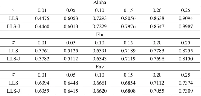
We add artificial noise with normal distribution N( , 2)where the mean  and the 0 standard deviation . The vertical axe indicates the NRMSE of each input scheme, and the horizontal axe represents the different level of standard deviation 0.01, 0.05, 0.1, 0.15, 0.2, 0.25.

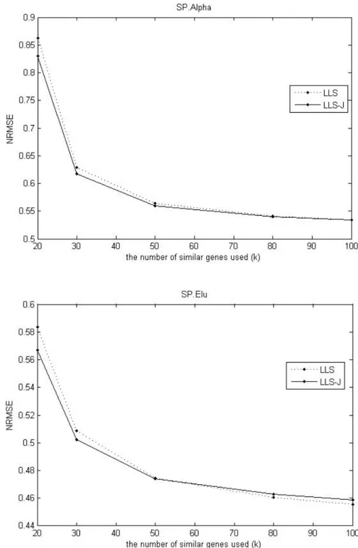
Fig. 1. Comparison of the NRMSEs of two methods and the effect of the number of genes for estimating missing values on SP.Alpha dataset and SP.Elu dataset.

In Figure 1, we find that the James-Stein approach shows better performance than LLSimpute when the k -value is small on SP.Alpha and SP.Elu datasets. When k is small, the James-Stein based method improves the conventional imputation.

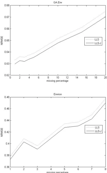
Fig. 2. Comparison of the NRMSEs of two methods and the effect of the number of genes for estimating missing values on GA.Env dataset and Environ dataset.

As shown in Figure 2, the James-Stein approach has better performance than LLSimpute both on GA.Env and Environ dataset.

In Figures 1and 2, we conclude that James-Stein approach improve LLSimpute when k is small on these four datasets.

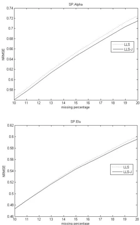
Fig. 3. Comparison of the NRMSEs against percentage of missing entries for two methods on SP.Alpha dataset and GA.Elu dataset.

In Figure 3, we compare NRMSE these imputations in the high level missing percentage. The James-Stein approach shows better performance on the SP.Alpha dataset and it performs better on the 15-20% missing on the SP.Elu dataset.

Fig. 4. Comparison of the NRMSEs against percentage of missing entries for two methods on Env dataset and Environ dataset.

In Figure 4, we find the James-Stein approach has good performance on both the GA.Env dataset and Environ dataset. In virtue of Figure 3 and 4, The James-Stein approach improves LLSimpute as the missing percentage increasing on the above datasets.

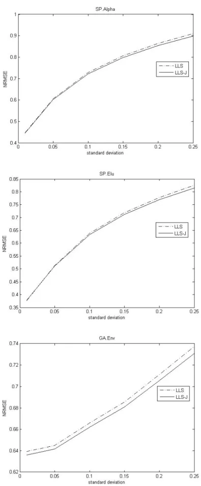
Fig. 5. Comparison of the NRMSEs with respect to noise levels on SP.Alpha dataset, SP.Elu dataset, and GA.Env dataset.

In Figure 5, to show how the methods respond to higher noise levels, we add some artificial noise by random normal distribution with different standard deviation. The Figure 5 shows that James-Stein approach improves LLSimpute efficiently on these datasets.

5.4

Simulation results for other imputations

In this section, we compare the performance of LLSimpute, SLLSimpute, ILLSimpute and the James-Stein approach for these methods on the SP.Alpha and GA.Env datasets; however, there is one problem with ILLSimpute. Among the comparison, ILLSimpute has some situation with serious estimation error such that the NRMSE value is large. The following figure is one of examples. The figure is to compare LLSimpute, SLLSimpute, ILLSimpute, and James-Stein approach with different missing percentage on SP.Alpha and GA.Env dataset.

There are some sharps on the curve of ILLSimpute on the above figures. We find ILLSimpute leads to worse estimates on some situations; however, other imputations perform stably at the same time. We delete the point where ILLSimpute has serious error to compare the different methods.

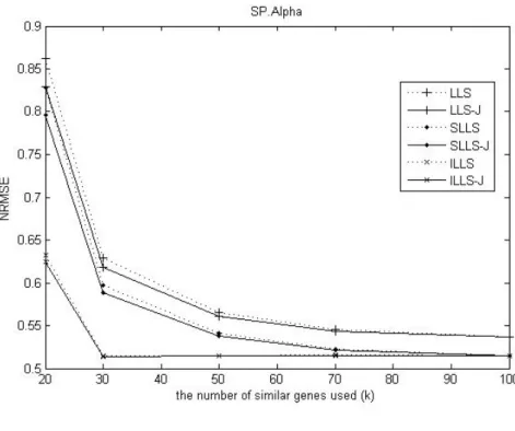
Fig. 6. NRMSEs comparison of four methods respect to the number of genes for estimating missing values on SP.Alpha dataset and GA.Env dataset.

As shown in Figure 6, SLLSimpute and ILLSimpute have smaller NRMSE than that of LLSimpute, revealing SLLSimpute and ILLSimpute are better than LLSimpute overall. In addition, the James-Stein estimator based methods efficiently improve these three imputations for small k.

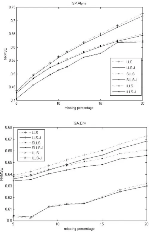
Fig. 7. Comparison of the NRMSEs against percentage of missing entries for two methods on Alpha dataset and Env dataset.

In Figure 7, ILLSimpute has better performance than LLSimpute and SLLSimpute.

In addition, James-Stein estimator based method can improve these three imputations efficiently as the missing percentage increases.

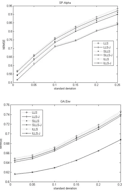
Fig. 8 Comparison of the NRMSEs of four methods with respect to noise levels on Alpha dataset and Env dataset.

In Figure 8, we find that these three imputations have worse performance as the artificial noise’s standard deviation increase. However, the James-Stein based method for these three imputations performance better overall. We conclude the James-Stein based method is less sensitive to the noise level.

6. Conclusion

Efficient imputation of missing values is needed for the using of microarray data, since most of downstream analyses require a complete dataset. Therefore, exploring accurate and efficient methods for estimating missing values has become a more important issue. In our studies, a shrinkage estimator method associated with a regression model is proposed to estimate missing values on microarray data. Our method takes advantage of the correlation structures existing in microarray data and selects similar genes for the target gene by Pearson correlation coefficients. Furthermore, we incorporate the least squares principle and utilize the James-Stein estimator to adjust the coefficients of the least squared estimation in the regression model to estimate missing values. A simulation study demonstrated that shrinkage estimator based method provided superior estimation accuracy for various types of datasets compared with LLSimpute and SLLSimpute when the k-value is less than 50. Since our proposed method can apply to any regression model based method and can provide better missing value estimation, it is a competitive alternative to the conventional least squares method.

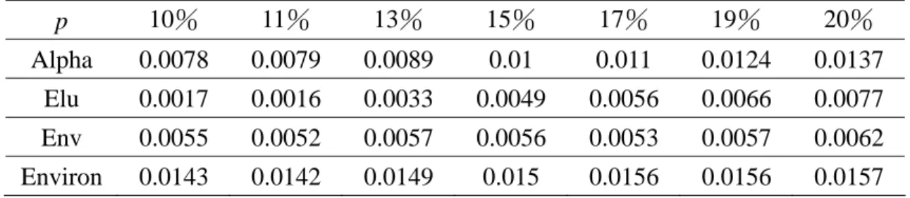
Table 1 Improvement ratio against specific percentage (p %) of missing entries p 10％ 11％ 13％ 15％ 17％ 19％ 20％ Alpha 0.0078 0.0079 0.0089 0.01 0.011 0.0124 0.0137 Elu 0.0017 0.0016 0.0033 0.0049 0.0056 0.0066 0.0077 Env 0.0055 0.0052 0.0057 0.0056 0.0053 0.0057 0.0062 Environ 0.0143 0.0142 0.0149 0.015 0.0156 0.0156 0.0157

Table 2 the NRMSEs against specific percentage (p %) of missing entries Alpha p 10％ 11％ 13％ 15％ 17％ 19％ 20％ LLS 0.5652 0.5819 0.6192 0.6526 0.6830 0.7124 0.7250 LLS-J 0.5608 0.5773 0.6137 0.6461 0.6755 0.7036 0.7151 Elu p 10％ 11％ 13％ 15％ 17％ 19％ 20％ LLS 0.4739 0.4890 0.5187 0.5461 0.5676 0.5900 0.6001 LLS-J 0.4731 0.4882 0.5170 0.5434 0.5644 0.5861 0.5955 Env p 1％ 2％ 3％ 4％ 5％ 10％ 15％ LLS 0.6333 0.6359 0.6355 0.6375 0.6390 0.6515 0.6611 LLS-J 0.6298 0.6326 0.6319 0.6339 0.6356 0.6478 0.6570 Environ p 1％ 2％ 3％ 5％ 6％ 7％ 8％ LLS 0.3783 0.4087 0.3964 0.4344 0.4371 0.4495 0.4776 LLS-J 0.3729 0.4029 0.3905 0.4279 0.4303 0.4425 0.4701

Table 3 Improvement ratio against different number of similar genes (k)

k 20 30 50 80 100

Alpha 0.0382 0.0185 0.0071 0.0017 0

Elu 0.0279 0.0124 0.0011 -0.0046 -0.0068

Env 0.0299 0.0152 0.0059 0.0009 -0.001

Table 4 the NRMSEs against different number of similar genes (k) Alpha k 20 30 50 80 100 LLS 0.8629 0.6286 0.5637 0.5412 0.535 LLS-J 0.8299 0.6170 0.5597 0.5403 0.535 Elu k 20 30 50 80 100 LLS 0.5834 0.5086 0.4744 0.4608 0.4556 LLS-J 0.5671 0.5023 0.4739 0.4629 0.4587 Env k 20 30 50 80 100 LLS 0.7888 0.6951 0.6489 0.6335 0.6283 LLS-J 0.7652 0.6845 0.6451 0.6329 0.6289 Environ k 10 20 30 50 100 LLS 0.3719 0.4444 0.6602 0.7305 0.4312 LLS-J 0.3697 0.4387 0.6478 0.7158 0.4246

Table 5 Improvement ratio against artificial noise with different standard deviations ( )

 0.01 0.05 0.10 0.15 0.20 0.25

Alpha 0.0034 0.0066 0.0088 0.0099 0.0105 0.0118

Elu -0.0056 0.0025 0.0075 0.0097 0.0112 0.0127

Env 0.0055 0.0051 0.0062 0.0067 0.0080 0.0088

Table 6 the NRMSEs against artificial noise with different standard deviations ( )

Alpha  _{0.01 0.05 0.10 0.15 0.20 0.25} LLS 0.4475 0.6053 0.7293 0.8056 0.8638 0.9094 LLS-J 0.4460 0.6013 0.7229 0.7976 0.8547 0.8987 Elu  _{0.01 0.05 0.10 0.15 0.20 0.25} LLS 0.3761 0.5125 0.6391 0.7189 0.7783 0.8255 LLS-J 0.3782 0.5112 0.6343 0.7119 0.7696 0.8150 Env  0.01 0.05 0.10 0.15 0.20 0.25 LLS 0.6394 0.6448 0.6661 0.6854 0.7112 0.7374 LLS-J 0.6359 0.6415 0.6620 0.6808 0.7055 0.7309

Table 7 Improvement ratio against specific percentage (p %) for three imputations. p 5％ 7％ 10％ 11％ 13％ 15％ 17％ 20％ LLS 0.0043 0.0058 0.0076 0.0079 0.0087 0.0098 0.0111 0.0132 SLLS 0.0019 0.0041 0.0057 0.0058 0.0060 0.0066 0.0070 0.0083 Alpha ILLS -0.0044 -0.0004 0.0006 0.0009 0.0030 0.0029 0.0187 0.0050 LLS 0.0052 0.0055 0.0057 0.0058 0.0056 0.0061 0.0059 0.0065 SLLS 0.0055 0.0064 0.0061 0.0060 0.0063 0.0077 0.0068 0.0073 Elu ILLS -0.0017 -0.0017 0.0008 0.0385 0.0005 0.0018 0.0024 0.0035

Table 8 the NRMSEs against specific percentage (p %) for three imputations. Alpha p 5％ 7％ 10％ 11％ 13％ 15％ 17％ 20％ LLS 0.4369 0.4966 0.5653 0.5842 0.6191 0.6506 0.6817 0.7270 LLS-J 0.4350 0.4937 0.5610 0.5796 0.6137 0.6442 0.6741 0.7174 SLLS 0.4291 0.4844 0.5410 0.5559 0.5832 0.6065 0.6268 0.6501 SLLS-J 0.4283 0.4824 0.5379 0.5527 0.5797 0.6025 0.6224 0.6447 ILLS 0.4049 0.4580 0.5147 0.5274 0.5634 0.5785 0.7972 0.6232 ILLS-J 0.4067 0.4582 0.5144 0.5269 0.5617 0.5768 0.7823 0.6201 Env p 5％ 7％ 9％ 11％ 13％ 15％ 17％ 20％ LLS 0.6392 0.6422 0.6472 0.6521 0.6565 0.6602 0.6658 0.6728 LLS-J 0.6359 0.6387 0.6435 0.6483 0.6528 0.6562 0.6619 0.6684 SLLS 0.6379 0.6397 0.6442 0.6474 0.6507 0.6532 0.6575 0.6608 SLLS-J 0.6344 0.6356 0.6403 0.6435 0.6466 0.6482 0.6530 0.6560 ILLS 0.6036 0.6023 0.6125 0.9456 0.6152 0.6210 0.6266 0.6321 ILLS-J 0.6046 0.6033 0.6120 0.9092 0.6149 0.6199 0.6251 0.6299

Table 9 Improvement ratio against different number (k) for three imputations.

k 20 30 50 70 100 LLS 0.0380 0.0186 0.0078 0.0031 0 SLLS 0.0393 0.0154 0.0055 0.0013 0 Alpha ILLS 0.0117 0.0014 0.0117 0.0010 0.0111 LLS 0.0302 0.0156 0.0057 0.0017 0 SLLS 0.0298 0.0161 0.0061 0.0027 0 Elu ILLS 0.0097 0.0458 0.0007 -0.0002 0.0016

Table 10 the NRMSEs against different number of similar genes selected (k) Alpha k 20 30 50 70 100 LLS 0.8624 0.6295 0.5653 0.5454 0.537 LLS-J 0.8296 0.6178 0.5609 0.5437 0.537 SLLS 0.8285 0.5976 0.5409 0.5224 0.515 SLLS-J 0.7959 0.5884 0.5379 0.5217 0.515 ILLS 0.6320 0.5148 0.6320 0.5155 0.632 ILLS-J 0.6246 0.5141 0.6246 0.5150 0.625 Env k 20 30 50 70 100 LLS 0.7935 0.6937 0.6492 0.6334 0.627 LLS-J 0.7695 0.6829 0.6455 0.6323 0.627 SLLS 0.7853 0.6894 0.6445 0.6300 0.623 SLLS-J 0.7619 0.6783 0.6406 0.6283 0.623 ILLS 0.6816 1.5308 0.6120 0.6074 0.615 ILLS-J 0.6750 1.4607 0.6116 0.6075 0.614

Table 11 Improvement ratio against artificial noise with different standard deviations ( ) for

three imputations.  0.01 0.05 0.1 0.15 0.2 0.25 LLS 0.0072 0.0080 0.0096 0.0106 0.0118 0.0131 SLLS 0.0066 0.0102 0.0108 0.0109 0.0116 0.0125 Alpha ILLS 0.0014 0.0108 0.0553 0.0064 0.0072 0.0067 LLS 0.0057 0.0059 0.0063 0.0069 0.0078 0.0090 SLLS 0.0059 0.0064 0.0069 0.0075 0.0081 0.0094 Elu ILLS 0.0018 0.0096 0.0002 -0.0008 -0.0009 -0.0003

Table 12 the NRMSEs against artificial noise with different standard deviations ( ) Alpha  0.01 0.05 0.1 0.15 0.2 0.25 LLS 0.5682 0.6610 0.7610 0.8288 0.8846 0.9335 LLS-J 0.5641 0.6557 0.7537 0.8200 0.8742 0.9213 SLLS 0.5449 0.6397 0.7422 0.8086 0.8641 0.9115 SLLS-J 0.5413 0.6332 0.7342 0.7998 0.8541 0.9001 ILLS 0.5166 0.6126 3.7703 0.7499 0.8075 0.8462 ILLS-J 0.5159 0.6060 3.5619 0.7451 0.8017 0.8405 Env  0.01 0.05 0.1 0.15 0.2 0.25 LLS 0.6489 0.6556 0.6717 0.6955 0.7186 0.7466 LLS-J 0.6452 0.6517 0.6675 0.6907 0.7130 0.7399 SLLS 0.6451 0.6523 0.6690 0.6923 0.7151 0.7439 SLLS-J 0.6413 0.6481 0.6644 0.6871 0.7093 0.7369 ILLS 0.6172 0.6847 0.6296 0.6447 0.6645 0.6877 ILLS-J 0.6161 0.6781 0.6295 0.6452 0.6651 0.6879

Reference:

1. Schena M, S.D., Davis RW, Brown PO, Quantitative monitoring of gene expression

patterns with a complementary DNA microarray. Science, 1995. 270: p. 467–470.

2. DeRisi JL, I.V., Brown PO, Exploring the metabolic and genetic control of gene

expression on a genomic scale. Science 1997. 278: p. 680–686.

3. Spellman PT, S.G., Zhang MQ, Iyer VR, Anders K, Eisen MB, Brown PO, Botstein D,

Futcher B, Comprehensive identification of cell cycle-regulated genes of the yeast

Saccharomyces cerevisiae by microarray hybridization. Mol Biol Cell 1998 9: p.

3273–3297.

4. Wu WS, L.W., Chen BS, Computational reconstruction of transcriptional regulatory

modules of the yeast cell cycle. BMC Bioinformatics, 2006. 7: p. 421.

5. Gasch AP, S.P., Kao CM, Carmel-Harel O, Eisen MB, Storz G, Botstein D, Brown PO,

Genomic expression programs in the response of yeast cells to environmental changes.

Mol Biol Cell 2000. 11: p. 4241–4257.

6. Wu WS, L.W., Identifying gene regulatory modules of heat shock response in yeast.

BMC Genomics 2008. 9: p. 439.

7. Chu, S., DeRisi,J., Eisen,M.B., Mulholland,J., Botstein,D., Brown,P.O. and

Hesrkowitz,I., The transcriptional program of sporulation in budding yeast. Science 1998. 278: p. 680-686.

8. Alizadeh, A.A., Eisen,M.B., Davis,R.E., Ma,C., Lossos,I.S., Rosenwald,A.,

Boldrick,J.C., Sabet,H., Tran, T, Powell,J.L. et al., Distinct types of diffuse large B-cell

lymphoma identified by gene expression profiling. Nature, 2000. 403: p. 503-511.

9. Ouyang, M.e.a., Gaussian mixture clustering and imputation of microarray data. .

Bioinformatics 2004. 20: p. 917–923.

10. Troyanskaya, O.e.a., Missing value estimation methods for cDNA microarrays. .

Bioinformatics 2001. 17: p. 520–525.

11. Schafer, J., Graham, J., Missing data: our view of the state of the art. Psychol.

Methods 2002. 7: p. 147–177.

12. Oba S, S.M., Takemasa I, Monden M, Matsubara K, Ishii S., A Bayesian missing value

estimation method for gene expression profile data. Bioinformatics. , 2003. 19(16): p.

2088-96.

13. Sehgal MS, G.I., Dooley LS., Collateral missing value imputation: a new robust

missing value estimation algorithm for microarray data. Bioinformatics. , 2005. 21(10): p. 2417-23.

14. Wang X, L.A., Jiang Z, Feng H., Missing value estimation for DNA microarray gene

expression data by Support Vector Regression imputation and orthogonal coding scheme. BMC Bioinformatics., 2006. 7: p. 32.

framework and biological knowledge. Nucleic Acids Res. , 2006 34(5): p. 1608-19.

16. Bø TH, D.B., Jonassen I., LSimpute: accurate estimation of missing values in

microarray data with least squares methods. Nucleic Acids Res., 2004. 32(3).

17. Kim H, G.G., Park H., Missing value estimation for DNA microarray gene expression

data: local least squares imputation. Bioinformatics. , 2005. 21(2): p. 187-98.

18. Cai Z, H.M., Lin G., Iterated local least squares microarray missing value imputation. J Bioinform Comput Biol., 2006 4(5): p. 935-57.

19. Ching WK, L.L., Tsing NK, Tai CW, Ng TW, Wong AS, Cheng KW., A weighted local

least squares imputation method for missing value estimation in microarray gene expression data. Int J Data Min Bioinform. , 2010. 4(3): p. 331-47.

20. Zhang X, S.X., Wang H, Zhang H., Sequential local least squares imputation

estimating missing value of microarray data. Comput Biol Med., 2008. 38(10): p.

1112-20.

21. Alter, O., Brown, P.O. and Botstein, D., Singular value decomposition for

genome-wide expression data processing and modeling. Proc. Natl Acad. Sci. USA,

2000. 97: p. 10101-10106.

22. Copas, J.B., Regression, Prediction and Shrinkage. J ROY STAT SOC B MET, 1983.

45(3): p. 311–354.

23. Stein, C., Inadmissibility of the Usual Estimator for the Mean of a Multivariate

Normal Distribution. Proc. Third Berkeley Symp. on Math. Statist. and Prob, 1956. 1:

p. 197-206.

24. W. James, a.C.S., Estimation with Quadratic Loss. Proc. Fourth Berkeley Symp. Math.

Statist. Prob, 1961. 1: p. 361–379.

25. Wang, H., Brown's paradox in the estimated confidence approach. ANN STAT 1999.

27: p. 610-626.

26. Wang, H., Improved confidence estimators for the multivariate normal confidence set.

STAT SINICA, 2000. 10: p. 659-664.

27. Gasch, A.P., Huang, M., Metzner, S., Botstein, D., Elledge, S.J.,Brown, P.O.,

Genomic expressipn response to DNA-damaging agents and the regulator role of the yeast ATR homolog Meclp. Mol Biol Cell, 2001. 12: p. 2987-3003