階層式光交換器光纖網路中的虛擬拓樸重置

全文

(1)國立交通大學資訊科學系碩士論文. 階層式光交換器光纖網路中的虛擬拓樸重置 Virtual Topology Reconfiguration in Hierarchical Cross-Connect WDM Networks. 研究生：葉筱筠指導教授：陳. 健教授. 中華民國九十三年六月.

(2) 階層式光交換器光纖網路中的虛擬拓樸重置 Virtual Topology Reconfiguration in Hierarchical Cross-Connect WDM Networks. 研究生：葉筱筠. Student：Hsiao-Yun Yeh. 指導教授：陳. Advisor：Chien Chen. 健. 國立交通大學資訊科學系碩士論文. A Thesis Submitted to Department of Computer and Information Science College of Electrical Engineering and Computer Science National Chiao Tung University in partial Fulfillment of the Requirements for the Degree of Master in Computer and Information Science June 2004 Hsinchu, Taiwan, Republic of China. 中華民國九十三年六月.

(3) 階層式光交換器光纖網路中的虛擬拓樸重置. 研究生 : 葉筱筠. 國. 立. 指導教授: 陳. 交. 通. 大. 學. 資. 訊. 科. 學. 健. 系. 摘要. 隨著資訊量的成長，光交換器的通道數也逐漸增長，造成光交換器的尺寸過大而不易製造與維護。因此階層式光交換器被提出來降低傳統交換器的成本、解決擴充性的問題及管理多單位的資訊流量。雖然在分波多工光纖網路上已經有許多關於虛擬拓樸重置的研究被提出來，這些研究都是考慮以傳統光交換器為架構的網路而尚未以階層式光交換器為架構來研究。在這篇論文中，我們以階層式光交換器為網路節點的架構以至於能有效的安排網路資源，並針對靜態及動態改變的資訊流量，提出一些方法來解決虛擬拓樸重置的問題。當未來的資訊流量變化可預期時，我們的研究方法是盡量保留現有虛擬拓樸中對未來流量有用處的虛擬鏈結，以減少對現有虛擬拓樸的破壞。另一方面，若資訊流量是隨時間動態變化且無法預期時，則中心管理者必須持續測量資訊流量並定期重置虛擬拓樸。模擬的結果驗證了在靜態流量變化的條件下，我們的重置策略藉由犧牲少許的阻塞機會大量的減少對虛擬拓樸的破壞。模擬結果也顯示在動態流量變化的條件下，當網路節點是傳統光交換器時，我們的方法能平衡虛擬鏈結上的流量；當網路節點是階層式光交換器時，我們的方法能有效的降低阻塞機會。. 關鍵字：虛擬拓樸重建、階層式光交換器、分波多工光纖網路。. i.

(4) Virtual Topology Reconfiguration in Hierarchical Cross-Connect WDM Networks. Student: Hsiao-Yun Yeh. Advisor: Dr. Chien Chen. Institute of Computer and Information Science National Chiao Tung University. Abstract With the growth in traffic, the number of ports needed at OXCs is growing, resulting in the size of OXCs too large to implement and maintain. Thus, hierarchical optical cross-connects (OXCs) are proposed for cost reduction, better scalability in physical size, and management of multigranularity traffics. Although virtual topology reconfiguration problem for a wavelength division multiplexing based optical network has been addressed by several previous studies, the node architectures of these studies are all traditional OXCs not hierarchical OXCs. In this thesis, we present some approaches to the virtual topology reconfiguration problem based on this kind of hierarchical OXCs under static and dynamic traffic demands so that network resources are arranged cost-effectively. When the future traffic is predicted, our approach is designed to reserve the useful existent virtual links for new traffic as much as possible and reduce the disruption of current virtual topology. On the other hand, if traffic dynamically changes without any predicted information about the future traffic pattern, a central manager must measure the traffic load on each virtual link continuously and reconfigure the virtual topology periodically. The simulation ii.

(5) results validate that our reconfiguration policies reduce lots of disruption under static traffic pattern at the cost of little blocking rate. The results also show that we balance the load of each virtual link with traditional OXC nodes and reduce the blocking rate with MG-OXC nodes under dynamic traffic pattern.. Keywords: hierarchical optical cross-connects, virtual topology reconfiguration, WDM networks.. iii.

(6) 誌謝本篇論文的完成，我要感謝這兩年來給予我協助與勉勵的人。首先要感謝我的指導教授陳健博士，陳老師對我的指導與教誨使我能在遇到困難時另尋突破，在研究上處處碰壁時指引明路讓我得以順利完成本篇論文，在此表達最誠摯的感謝。同時也感謝我的論文口試委員，交大的王國禎教授、清大的陳志成教授、以及工研院的李詩偉博士，他們提出了許多的寶貴意見。. 感謝生命共同體的成員陳盈羽及羅澤羽，由於他們與我的互相討論及在論文上的協助，使我的研究更為完善。另外我也要感謝實驗室的學長、同學、學弟們，吳奕緯、許嘉仁、官政佑、林俊源、王獻綱、徐勤凱、陳咨翰以及劉上群等人，他們的陪伴及支持讓我在風雨中能夠堅持下去。. 感謝我的室友，鄭佩琪、葉桂如、張嘉玲，他們在精神上給我莫大的鼓勵，傾聽我內心的聲音並帶給我無比的溫暖，這些好朋友們的聲音陪伴我度過枯燥的研究生涯。. 最後，我要感謝我的家人對我的關懷及支持，含辛茹苦的培養我得以唸至研究所，我要向他們致上最高的感謝。. iv.

(7) Table of Content Abstract (In Chinese)....................................................................................................i Abstract.........................................................................................................................ii Acknowledgement (In Chinese) .................................................................................iv Table of Content ...........................................................................................................v List of Figures..............................................................................................................vi List of Tables............................................................................................................. viii Chapter 1: Introduction ..............................................................................................1 Chapter 2: Reconfiguration Scheme for Static Traffic in Hierarchical Cross-connect WDM Networks ..................................................................................6 2.1 Introduction......................................................................................................6 2.2 Previous Work..................................................................................................7 2.3 Assumptions.....................................................................................................7 2.4 Preference Based Reconfiguration Algorithm for Static Traffic (PBRAST) ...8 2.5 Numerical Results..........................................................................................14 2.5.1 Simulation Environment .....................................................................14 2.5.2 Simulation Results ..............................................................................16 Chapter 3: Reconfiguration Issue for Dynamic Traffic in Hierarchical Cross-connect WDM Networks ................................................................................20 3.1 Introduction....................................................................................................20 3.2 The heuristic adaptation algorithm in [13].....................................................21 3.3 Heuristic Algorithms for Dynamic Traffic in Traditional OXC Networks ....22 3.3.1 Rerouting Based Reconfiguration Algorithm for Dynamic Traffic (RBRADT)...................................................................................................23 3.3.2 Weighted Based Reconfiguration Algorithm for Dynamic Traffic (WBRADT)..................................................................................................26 3.4 A Heuristic Algorithm for Dynamic Traffic in MG-OXC Networks.............28 3.5 Numerical Results..........................................................................................31 3.5.1 Performance Analysis .........................................................................31 3.5.2 Simulation Environment .....................................................................32 3.5.3 Simulation Results ..............................................................................33 Chapter 4: Conclusions and Future Works.............................................................43 Reference: ...................................................................................................................45. v.

(8) List of Figures Fig. 1. A virtual topology is designed for the given traffic load1 ...................................2 Fig. 2. An example of virtual topology reconfiguration ................................................3 Fig. 3. Architecture of an MG-OXC ..............................................................................4 Fig. 4. Illustration of the construction of auxiliary graph ............................................10 Fig. 5. Illustration of calculating CL. (a) Conflictions happen at physical links and at end nodes. (b) A detailed drawing of the confliction at the end nodes. ....................... 11 Fig. 6. Cost definition for edges in Ga .........................................................................12 Fig. 7. Computation of W.............................................................................................13 Fig. 8. Preference Based Reconfiguration Algorithm for Static Traffic ......................14 Fig. 9. The physical topology of our simulation environment.....................................15 Fig. 10. Combination of different traffic patterns with 1F2B2L .................................17 Fig. 11. Combination of different traffic patterns with 2F1B2L..................................18 Fig. 12. Combination of different traffic patterns with 2F2B1L .................................19 Fig. 14. Rerouting Based Reconfiguration Algorithm for Dynamic Traffic................25 Fig. 15. Example for calculating weight matrix M ......................................................27 Fig. 16. Weighted Based Reconfiguration Algorithm for Dynamic Traffic.................28 Fig. 17. Illustration of calculating CL. (a) Conflictions happen at physical links and at end nodes. (b) A detailed drawing of the confliction at the end nodes. .......................30 Fig. 18. Periodic Tunnel Reconfiguration Algorithm for Dynamic Traffic .................31 Fig. 19. Illustration of five traffic rate functions .........................................................33 Fig. 20. Maximal lightpath load with high watermark=0.75 and period=400 time units, (a) is the algorithm in [13], (b) is RBRADT and (c) is WBRADT..............................36 Fig. 21. Impulse graphic indicating times of lightpath addition or deletion with high watermark=0.75 and period=400 time units, (a) is the algorithm in [13], (b) is RBRADT and (c) is WBRADT....................................................................................36 Fig. 22. Maximal lightpath load with high watermark=0.75 and period=200 time units, (a) is the algorithm in [13], (b) is RBRADT and (c) is WBRADT..............................37 Fig. 23. Impulse graphic indicating times of lightpath addition or deletion with high watermark=0.75 and period=200 time units, (a) is the algorithm in [13], (b) is RBRADT and (c) is WBRADT....................................................................................37 Fig. 24. Maximal lightpath load in network with high watermark=0.75 and period=100 time units, (a) is the algorithm in [13], (b) is RBRADT and (c) is WBRADT. ...................................................................................................................38 Fig. 25. Impulse graphic indicating times of lightpath addition or deletion with high watermark=0.75 and period=100 time units, (a) is the algorithm in [13], (b) is RBRADT and (c) is WBRADT....................................................................................38 Fig. 26. Maximal lightpath load and adjustments with high watermark=0.85 and vi.

(9) period=400 time units. (a) and (c) are RBRADT. (b) and (d) are WBRADT..............39 Fig. 27. Maximal lightpath load and adjustments with high watermark=0.65 and period=400 time units. (a) and (c) are RBRADT. (b) and (d) are WBRADT..............39 Fig. 28. Blocking probability of 1F2B2L when each fiber has ten wavelengths.........40 Fig. 29. Blocking probability of 2F1B2L when each fiber has ten wavelengths.........40 Fig. 30. Blocking probability of 2F2B1L when each fiber has ten wavelengths.........41 Fig. 31. Blocking probability of 1F2B2L when each fiber has twenty wavelengths...41 Fig. 32. Blocking probability of 2F1B2L when each fiber has twenty wavelengths...42 Fig. 33. Blocking probability of 2F2B1L when each fiber has twenty wavelengths...42. vii.

(10) List of Tables Table I Cost Definition for Edges in Ga ……………………………………….……10 Table II Time Complexity Comparisons between [13], RBRADT and WBRADT…32. viii.

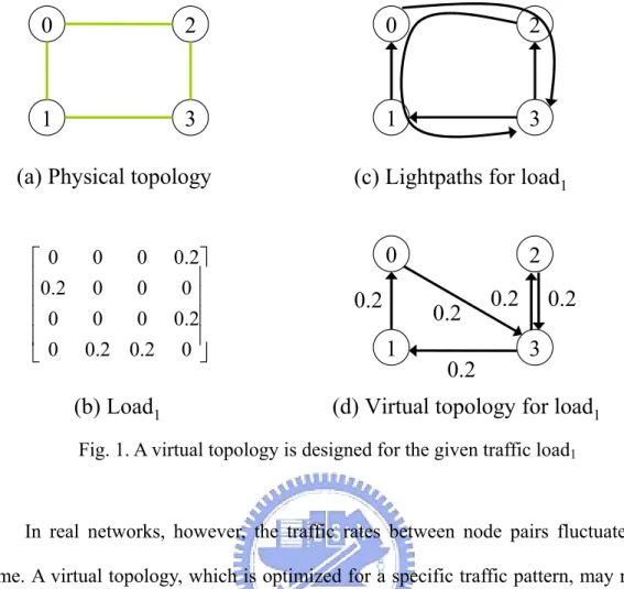
(11) Chapter 1: Introduction All-optical wavelength-division-multiplexed (WDM) networks are considered to be one of the most promising transport infrastructures to solve the huge bandwidth demands. The network is composed of optical cross-connects (OXCs) interconnected by fiber links, with each fiber provides a number of wavelength channels. Traffic in the network is transmitted via all-optical WDM channels, referred to as lightpaths. A lightpath may span a number of fiber links to provide a “circuited switched” interconnection between two nodes without undergoing electronic processing at intermediate nodes. In the absence of wavelength converters, a lightpath has to operate on the same wavelength along its route, which is known as the wavelength continuity constraint. Using wavelength converters, a lightpath may use different wavelengths on its route from its source to its destination. A virtual topology is defined to be the set of such lightpaths in a network. Design of virtual topology is the problem of optimizing the use of network resources for the given traffic demands among all node pairs. This problem has been addressed by several previous studies and a literature survey can be found in [1]. Fig. 1 illustrates the concept of virtual topology. There are four nodes and four links in the physical topology (Fig. 1(a)). Assume each link is bidirectional with each direction contains a fiber and a fiber has only one wavelength. For a given traffic load1 (Fig. 1(b)), we design a virtual topology (Fig. 1(d)) formed by a set of lightpaths (Fig. 1(c)) to minimize the maximum load of all virtual links.. 1.

(12) 0. 2. 0. 2. 1. 3. 1. 3. (a) Physical topology. (c) Lightpaths for load1 0. 0 0 0 .2 ⎤ ⎡0 ⎢ 0 .2 0 0 0 ⎥⎥ ⎢ ⎢0 0 0 0 .2 ⎥ ⎢ ⎥ ⎣ 0 0.2 0.2 0 ⎦. 0.2. 0.2 1. (b) Load1. 2. 0.2. 0.2. 0.2 3. (d) Virtual topology for load1. Fig. 1. A virtual topology is designed for the given traffic load1. In real networks, however, the traffic rates between node pairs fluctuate over time. A virtual topology, which is optimized for a specific traffic pattern, may not be able to respond with equal efficiency to a different traffic pattern. Therefore, it is necessary to change the virtual topology appropriately to reflect the new traffic pattern. This network adaptation operation is called reconfiguration process. Continue with the example in Fig. 1, let the traffic pattern changed to load2 (Fig. 2(a)). If we use the original virtual topology to serve load2, the load of each link will increase and congestion may happen at some virtual links with high loads (Fig. 2(b)). On the other hand, we can reconfigure the original virtual topology into a new virtual topology (Fig. 2(d)) formed by another set of lightpaths (Fig. 2(c)) and reroute load2 on it. Now the load of each virtual link is greatly decreased and no congestion will happen.. 2.

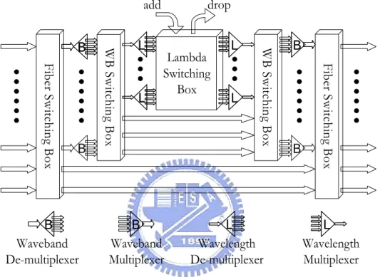
(13) 0⎤ ⎡ 0 0.2 0 ⎢0 0 0.2 0.2⎥⎥ ⎢ ⎢0.1 0.1 0 0⎥ ⎢ ⎥ 0 0.2 0 ⎦ ⎣0. 0.5 1. 0.4. 1. 3. 0. 2 0.6. 2. (c) Lightpaths for load2. (a) Load2. 0. 0. 0.2. 0.2. 0.4 0.2 3. 0.1 1. (b) Load2 on the original virtual topology. 0.1. 0.2. 2 0.2 3. (d) Load2 on the reconfigurable virtual topology. Fig. 2. An example of virtual topology reconfiguration. As the number of wavelength channel increases, the number of ports needed at OXC also increases, making the size of OXC too large to implement and maintain. For this reason, many hierarchical optical cross-connects, or multigranularity optical cross-connects (MG-OXCs) have been proposed to solve this scalability problem in [2], [3] and [4]. Although MG-OXCs are gaining more and more research attentions, not much is devoted on the virtual topology reconfiguration problem in the MG-OXC networks. In this thesis, we study the virtual topology reconfiguration problem in the networks with their node architecture being the MG-OXC proposed in [2].. The MG-OXC, shown in Fig. 3, mainly comprises fiber-, waveband-, and wavelength-switching boxes. With such MG-OXC, the switching types are no longer limited to wavelength-switched, but also waveband- or fiber-switched. In such network, a directional link consists of F fibers in which F1, F2, and F3 fibers are 3.

(14) assigned as fiber-switched, waveband-switched, and wavelength-switched fibers respectively (i.e. F = F1 + F2 + F3). A fiber/waveband tunnel can be set up by grouping a fiber/waveband of wavelengths and switch them as a single unit using fiber-/waveband-switched fibers until they are degrouped.. add. L. Lambda Switching Box. L. L. L Wavelength De-multiplexer. B Waveband Multiplexer. B. B. Fiber Switching Box. B Waveband De-multiplexer. L. WB Switching Box. Fiber Switching Box. B. WB Switching Box. B. drop. L Wavelength Multiplexer. Fig. 3. Architecture of an MG-OXC. In this thesis, we study the virtual topology reconfiguration problem for both static traffic and dynamic traffic in MG-OXC networks. Here the static traffic means that the future traffic pattern formed by lightpath requests is assumed to be known in advance while the dynamic traffic means that the traffic fluctuates over time and we do not know a priori the future traffic.. The remainder of the thesis is organized as follows. Chapter 2 presents the heuristics of virtual topology reconfiguration for static traffic in MG-OXC networks. Reconfiguration issue for dynamic traffic in hierarchical cross-connect WDM 4.

(15) networks are proposed in Chapter 3. Finally, conclusions and future works are summarized in Chapter 4.. 5.

(16) Chapter 2: Reconfiguration Scheme for Static Traffic in Hierarchical Cross-connect WDM Networks 2.1 Introduction This chapter studies the virtual topology reconfiguration problem for static traffic in MG-OXC networks. The static traffic means that the future traffic pattern is known in advance. Since the future traffic is expectable, we can know a priori how many lightpaths needed between the end nodes in the networks. Therefore, we assume that each request is for a lightpath. The virtual topology studied here is formed by the set of tunnels and the fiber links dedicated for wavelength-switching. We consider the following network design problem. Given T1, V1, and T2, where V1 is a set of tunnels allocated based on current traffic pattern T1 and T2 is the future traffic pattern, the objective is to reconfigure V1 with little changes as possible while minimizing the blocking probability for T2. We propose the heuristic, Preference Based Reconfiguration Algorithm for Static Traffic (PBRAST), which is based on an auxiliary graph used to rate the preference of each existent and nonexistent tunnel by routing T2 on it and then decide a set of tunnels according to the obtained preferences.. The remainder of this chapter is organized as follows. Section 2.2 briefly introduces previous work on reconfiguration problem for static traffic in traditional OXC networks. Section 2.3 then gives the assumptions made in this chapter. A heuristic for reconfiguration problem is presented in Section 2.4. Finally, simulation results are given in Section 2.5.. 6.

(17) 2.2 Previous Work. Previous work on virtual topology reconfiguration for static traffic is summarized as follows. Authors in [5] and [6] show the virtual topology reconfiguration using the mixed integer linear programming (MILP) formulation. The formulations ensure that the new configuration is not too different from the original virtual topology so that number of reconfiguration steps can be minimized.. In [7] and [8], the authors propose several reconfiguration algorithms that attempt shift from one virtual topology to another while keeping the disruption of the network minimum. They focus on the process of transforming the virtual topology from the original to the new one but not on finding the optimal virtual topology for the given network traffic pattern.. Other authors deal with virtual topology reconfiguration but their network topologies are limited to simple models such as local area network (LAN). In [9], [10], [11] and [12], they propose a sequence of steps involved in the transition of an optical network from one configuration to another. And these approaches change the network through a sequence of branch exchange or node exchange operation, so that only two or three links or the links connected with two nodes are disrupted at any given time.. 2.3 Assumptions. We consider a network with N nodes connected by bidirectional optical links forming a physical topology. Each optical link supports a fixed number of fibers, and each of fiber contains the same number of wavelengths. Each node is assumed to have 7.

(18) full wavelength conversion only for transition between different switching types. The tunnels are restricted to traverse only on their shortest paths from their ingress to egress node to efficiently utilize the network resources. A waveband (fiber) tunnel can be established between any node pair if the resources of waveband (fiber) layer are available along the path and ports of wavelength-switching layer at source and destination node are enough. Note that for the waveband tunnel, it has to use the same waveband on each link along the route. The number of wavelength-switching ports a tunnel consumes at the two ends of the tunnel is equal to the number of the wavelengths that the tunnel carries.. In this study, the tunnels are required to follow the tunnel length constraint, i.e., the length of each tunnel should be the same, which is set to the minimum integer that is larger than the average distance of paths between each s-d pair in the network [2]. This is because when the tunnel length is too small, although the short tunnels are flexible and easily utilized by most of the lightpaths, the wavelength-switching ports are used up easily since the wavelength-switching ports are required at the ingress and egress nodes of each tunnel. When the tunnel length is too large, although wavelength-switching ports can be greatly saved, the tunnels may not be suitable for the requests since most of the lightpath requests are shorter than the tunnels.. 2.4 Preference Based Reconfiguration Algorithm for Static Traffic (PBRAST). PBRAST is based on an auxiliary graph used to rate for each node pair the preference of having tunnels for it. Since the length constraint can be derived from the given physical topology, we can determine all the potential node pairs that could be 8.

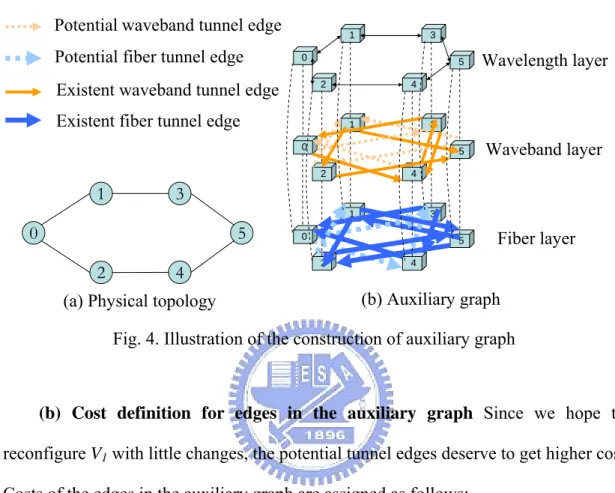
(19) allocated tunnels at the beginning. PBRAST first construct an auxiliary graph in which some of its edges represent the existent and nonexistent tunnels among those potential node pairs. The preferences for those tunnels are actually the estimated load on them and are rated by routing T2 on the auxiliary graph using the shortest path algorithm. The new set of tunnels, i.e. V2, are then determined according to the estimated preferences. The whole process comprises four stages: (a) construction of auxiliary graph, (b) cost definition for edges in the auxiliary graph, (c) load estimation of existent and nonexistent tunnels, and (d) tunnels selection. Details are described as follows.. (a) Construction of auxiliary graph Let Gp(Vp, Ep) be the physical topology where Vp denotes the set of nodes and Ep is the set of all physical links connecting the nodes. The auxiliary graph Ga(Va, Ea) is obtained as follows. Each node i ∈ Vp is replicated three times in Ga. These nodes are denoted as ViW, ViB and ViF ∈ Va. If edge e ∈ Ep connects node i to node j, i, j ∈ Vp, then node ViW is connected to VjW by a directed edge, termed wavelength-switching edge. For each node pair i-j with existent waveband (fiber) tunnel in V1, the node ViB (ViF) is connected to VjB (VjF) by a directed edge, termed existent waveband (fiber) tunnel edge. For each node pair i-j with its shortest physical hop length follow the length constraint and has not yet been allocated waveband (fiber) tunnel, there is also an edge connecting from ViB to VjB (ViF to VjF), termed potential waveband (fiber) edge. For each node i ∈ Vp, there are bidirectional edges between ViW, ViB, and ViF, termed layer transition edge.. Fig. 4 gives an example of construction of the auxiliary graph. Fig. 4(a) is the physical topology with its average hop distance equal to two. The corresponding auxiliary graph may be the one shown in Fig. 4(b) where the thick edges in the 9.

(20) waveband (fiber) layer represent the existent waveband (fiber) tunnel edges and the dash edges the potential waveband (fiber) tunnel edges.. Potential waveband tunnel edge Potential fiber tunnel edge. 1. 3. 0. Existent waveband tunnel edge. 2. Existent fiber tunnel edge. 1. 5. Waveband layer. 3. 2. 4. 3 1. 0. 5 2. Wavelength layer. 4. 0. 1. 5. 3. 0. 5 2. 4. Fiber layer. 4. (b) Auxiliary graph. (a) Physical topology. Fig. 4. Illustration of the construction of auxiliary graph. (b) Cost definition for edges in the auxiliary graph Since we hope to reconfigure V1 with little changes, the potential tunnel edges deserve to get higher cost. Costs of the edges in the auxiliary graph are assigned as follows:. Table I Cost Definition for Edges in Ga Existent waveband (fiber) tunnel edge. D (Length constraint). Potential waveband (fiber) tunnel edge D′ + scale Wavelength-switching edge. A Large number. Layer transition edges. 0. In order to give more preference to the existent tunnels when routing T2 on the auxiliary graph, the costs of the potential tunnel edges are higher than the existent 10.

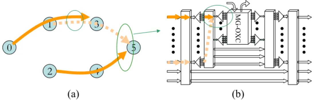
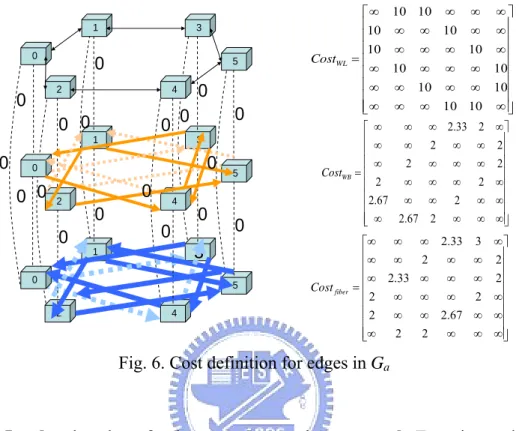
(21) tunnel edges. D′ is used to adjust the degree of preference on the existent tunnels where D′ ≥ D and D′ ∈ Z. The higher D′ we select, the higher degree of preference the existent tunnels have. For each potential waveband (fiber) edge, there is a scale associated with it. The scale represents the degree of difficulty to construct a tunnel for the node pair associated with that edge. The more existent tunnels must be deleted to construct a tunnel for a potential tunnel edge, the larger the scale for that potential tunnel edge. Scale for the potential tunnel edge i is defined as (CLi－CLmin) / (CLmax－ CLmin), where CLi is the number of existent tunnels that conflict with the construction of the tunnel for the node pair associated with i, CLmax =. CLmin =. min. j∈potential tunnel edges. max. j∈potential tunnel edges. CL j and. CL j . Figure 5 illustrates the calculation of CL for the potential. tunnel edge. The conflictions between the existent and nonexistent tunnels may happen at physical links and the end nodes of the tunnels. In Fig. 5(a), the thick and dash lines represent the actual physical paths of existent and nonexistent tunnels, respectively. The nonexistent tunnel (1, 5) conflicts with the existent tunnel (0, 3) at the physical link (1, 3) and with the existent tunnel (2, 5) at the end node 5 (Fig. 5(b)). Thus, the CL for the potential tunnel edge (1, 5) is 2.. MG-OXC. 1. 3. 0. 5 4. 2 (a). (b). Fig. 5. Illustration of calculating CL. (a) Conflictions happen at physical links and at end nodes. (b) A detailed drawing of the confliction at the end nodes.. Figure 6 is an example after setting the costs for all edges in the auxiliary graph. 11.

(22) In Fig. 6, the costs of the edges in wavelength layer, waveband layer, and fiber layer are recorded in the matrixes CostWL, CostWB, and Costfiber, respectively.. 1 0. 3. 0 2. 0. 4. 0 0. 0 0. 0 0 1. 0. 3. 0. 0. 0 0. CostWL. 5. 0. 2. 4. 0. 0 0. 0. CostWB. 5. 0. 3. 1 0. 5 2. Cost fiber. 4. ⎡ ∞ 10 10 ∞ ∞ ∞ ⎤ ⎢10 ∞ ∞ 10 ∞ ∞ ⎥ ⎥ ⎢ ⎢10 ∞ ∞ ∞ 10 ∞ ⎥ =⎢ ⎥ ⎢ ∞ 10 ∞ ∞ ∞ 10⎥ ⎢ ∞ ∞ 10 ∞ ∞ 10⎥ ⎥ ⎢ ⎣⎢ ∞ ∞ ∞ 10 10 ∞ ⎦⎥ ∞ ⎡ ∞ ⎢ ∞ ∞ ⎢ ⎢ ∞ 2 =⎢ 2 ∞ ⎢ ⎢2.67 ∞ ⎢ ⎢⎣ ∞ 2.67. ⎡∞ ∞ ⎢∞ ∞ ⎢ ⎢∞ 2.33 =⎢ ∞ ⎢2 ⎢2 ∞ ⎢ 2 ∞ ⎣⎢. ∞ 2.33 2 ∞ ⎤ 2 ∞ ∞ 2 ⎥⎥ ∞ ∞ ∞ 2⎥ ⎥ ∞ ∞ 2 ∞⎥ ∞ 2 ∞ ∞⎥ ⎥ 2 ∞ ∞ ∞ ⎥⎦. ∞ 2.33 3 ∞ ⎤ 2 ∞ ∞ 2 ⎥⎥ ∞ ∞ ∞ 2⎥ ⎥ 2 ∞⎥ ∞ ∞ ∞ 2.67 ∞ ∞ ⎥ ⎥ 2 ∞ ∞ ∞ ⎦⎥. Fig. 6. Cost definition for edges in Ga. (c) Load estimation of existent and nonexistent tunnels To estimate the load. of the existent and nonexistent tunnels, shortest path routing algorithm is applied to route T2 on the auxiliary graph. A weight matrix W is used to record the load for those existent and nonexistent tunnels. We assume that the load between each node pair will be equally distributed on all its shortest paths. For example, in Fig. 6, assume the future traffic between node 0 and node 5 is 10. Five shortest paths can be found as shown in Fig. 7(a). Therefore, each of the five paths is distributed 2 units of the load. The weight matrix is then updated as shown in Fig. 7(b) where W0,4 = 2, W1,5 = 2 + 2 = 4 and W2,5 = 2 + 2 = 4.. 12.

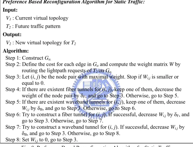
(23) 1. T(0, 5) = 10. 3. 0. Number of Path (0, 5) = 5. 5 2. Addition Weight = 10/5 = 2. 4. 1. 3. 0. ⎡0 ⎢0 ⎢ ⎢0 W =⎢ ⎢0 ⎢0 ⎢ ⎣⎢0. 5 2. 4. 1. 3. 0. 5 2. 4. (a). 0 0 0 2 0⎤ 0 0 0 0 4 ⎥⎥ 0 0 0 0 4⎥ ⎥ 0 0 0 0 0⎥ 0 0 0 0 0⎥ ⎥ 0 0 0 0 0 ⎦⎥. (b) Fig. 7. Computation of W. (d) Tunnels selection W is used to determine the set of tunnels. The process. repeatedly examine the node pair with the maximum weight to see whether there are existent tunnels for the node pair, otherwise, it tries to construct a new tunnel for the node pair. At the end of each repetition, weight of the chosen node pair is subtracted by a suitable value. The process ends until weight for each node pair is equal or less then zero. Details of the examination are as follows. If there are already existent tunnels allocated between the selected pair, keep one of them in the virtual topology. Otherwise, construct a tunnel between the selected pair and if necessary, delete the existent tunnels that hinder the construction. Note that whether keeping or constructing a tunnel, the fiber tunnel is considered first. If a fiber tunnel is kept, or constructed successfully, weight of the corresponding node pair is decreased by. δF =. ∑W. i, j. L ⋅ FT D. , where Wi,j is the weight of the node pair (i, j), L the number of. directional links in the physical topology, FT the number of fibers dedicated to tunnel allocation in each directional link and D the length constraint. Similarly, for the 13.

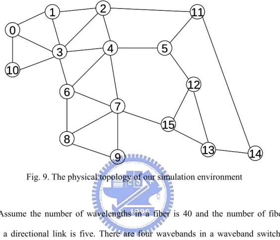
(24) waveband tunnel, the weight is decreased by δ B =. ∑W. i, j. L ⋅ B ⋅ FT D. , where B is the number. of wavebands in a fiber. If both fiber and waveband tunnels fail to be constructed, the weight is set to 0. The whole algorithm of PBRAST is summarized as follows.. Preference Based Reconfiguration Algorithm for Static Traffic: Input: V1 : Current virtual topology T2 : Future traffic pattern Output: V2 : New virtual topology for T2 Algorithm: Step 1: Construct Ga. Step 2: Define the cost for each edge in Ga and compute the weight matrix W by routing the lightpath requests of T2 on Ga. Step 3: Let (i, j) be the node pair with maximal weight. Stop if Wi,j is smaller or equal to 0. Step 4: If there are existent fiber tunnels for (i, j), keep one of them, decrease the weight of the node pair by δF, and go to Step 3. Otherwise, go to Step 5. Step 5: If there are existent waveband tunnels for (i, j), keep one of them, decrease Wi,j by δB, and go to Step 3. Otherwise, go to Step 6. Step 6: Try to construct a fiber tunnel for (i, j). If successful, decrease Wi,j by δF, and go to Step 3. Otherwise, go to Step 7. Step 7: Try to construct a waveband tunnel for (i, j). If successful, decrease Wi,j by δB, and go to Step 3. Otherwise, go to Step 8. Step 8: Set Wi,j to 0, go to Step 3. Fig. 8. Preference Based Reconfiguration Algorithm for Static Traffic. 2.5 Numerical Results 2.5.1 Simulation Environment. Simulation experiments were conducted to investigate the performance of our heuristic algorithms on the 16-node network shown in Fig. 9. The nodes of this network are interconnected by 27 bidirectional links. (F1)F(F2)B(F3)L represents the 14.

(25) experiment with F1 fibers for fiber switching, F2 fibers for waveband switching and F3 fibers for wavelength switching on each link.. 2. 1. 11. 0 4. 3. 5. 10 12. 6 7 15 8. 13. 9. 14. Fig. 9. The physical topology of our simulation environment. Assume the number of wavelengths in a fiber is 40 and the number of fibers along a directional link is five. There are four wavebands in a waveband switched fiber. Each waveband has ten wavelengths, with the first to the tenth wavelengths being in the first waveband, the 11th to the 20th wavelengths being in the second waveband, …, and the 31st to the 40th wavelengths being in the fourth waveband. Each traffic pattern consists of lightpath requests and after routing these lightpath requests on the network, the lightpaths will not leave the network. The traffic patterns are described as follows:. y Ring type traffic. Most traffic flows are from node i to node (i + 1), i = 0, …,14, and from node 15 to node 0.. 15.

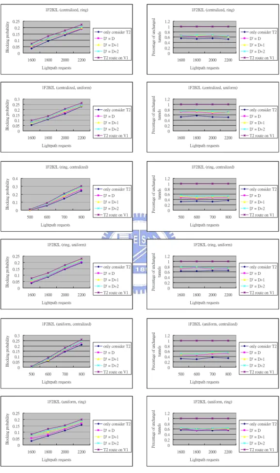
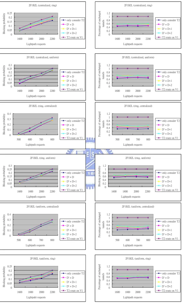
(26) y Centralized type traffic. Most traffic flows are from node 0 to other nodes. y Uniform traffic. All traffic flows are random generated between each node pair.. 2.5.2 Simulation Results. Figure 10~12 show the simulation results of all combinations with 1F2B2L, 2F1B2L, and 2F2B1L, respectively. The value of x-axis is the number of lightpath requests in T2. The y-axis on the left-hand charts of the Fig. 10~12 is the blocking probability and the y-axis on the right-hand charts of the Fig. 10~12 is percentage of unchanged tunnels on V1. We use different combinations of the types of the current and future traffic patterns represented by (T1, T2) with different D' ( D' = D, D+1, D+2) and different switching types of fibers. With each combination, the virtual topology that only considers T2 without considering V1 always keeps the lowest blocking probability and the lowest value of percentage of unchanged tunnels. However, when we route T2 on V1 without reconfiguration, the blocking probability is the highest and the value of the percentage of unchanged tunnels is a hundred per cent. When we apply PBRAST to reconfigure V1, if D' is higher, the percentage of unchanged tunnels and the blocking probability are also higher. Higher D' means that to construct a nonexistent tunnel is more difficult and more unchanged tunnels are left in V2. With the arising number of unchanged nonexistent tunnels in the new virtual topology, the blocking probability rate is arising, too. However, the arising blocking probability rates are still closed to the optimal value and the rise at some cases is even growing up to 40 % of original number of tunnels.. 16.

(27) 1F2B2L (centralized, ring). Percentage of unchanged tunnels. Blocking probability. 1F2B2L (centralized, ring) 0.25 0.2. only consider T2. 0.15. D' = D. 0.1. D' = D+1. 0.05. D' = D+2. 0 1600. 1800. 2000. 2200. T2 route on V1. 1.2 1 0.8 0.6 0.4 0.2 0. only consider T2 D' = D D' = D+1 D' = D+2. 1600. Lightpath requests. 0.3 0.25 0.2 0.15 0.1 0.05 0. only consider T2. D' = D. D' = D+1. D' = D+2 1800. 2000. 2200. T2 route on V1. only consider T2 D' = D+1 D' = D+2. 1600. only consider T2. 0.2. D' = D. 0.1. D' = D+1 D' = D+2. 0 800. T2 route on V1. D' = D D' = D+1 D' = D+2 500. only consider T2. 0.15. D' = D. 0.1. D' = D+1. 0.05. D' = D+2. 0 2200. T2 route on V1. only consider T2 D' = D+1 D' = D+2. 1600. Percentage of unchanged tunnels. Blocking probability. 2200. only consider T2 D' = D+1 D' = D+2. 800. T2 route on V1. 1.2 1 0.8 0.6 0.4 0.2 0. T2 route on V1. only consider T2. D' = D. D' = D+1. D' = D+2 500. 600. 700. 800. T2 route on V1. Lightpath requests. Lightpath requests. 1F2B2L (uniform, ring). 1F2B2L (uniform, ring) Percentage of unchanged tunnels. Blocking probability. 2000. 1F2B2L (uniform, centralized). D' = D. 0.25 0.2. only consider T2. 0.15. D' = D. 0.1. D' = D+1. 0.05. D' = D+2. 0 2000. 1800. Lightpath requests. 0.3 0.25 0.2 0.15 0.1 0.05 0. 1800. T2 route on V1. D' = D. 1F2B2L (uniform, centralized). 1600. 800. 1.2 1 0.8 0.6 0.4 0.2 0. Lightpath requests. 700. 700. 1F2B2L (ring, uniform) Percentage of unchanged tunnels. Blocking probability. 0.2. 600. 600. Lightpath requests. 0.25. 500. T2 route on V1. only consider T2. 1F2B2L (ring, uniform). 2000. 2200. 1.2 1 0.8 0.6 0.4 0.2 0. Lightpath requests. 1800. 2000. 1F2B2L (ring, centralized) Percentage of unchanged tunnels. Blocking probability. 0.3. 1600. 1800. Lightpath requests. 0.4. 700. T2 route on V1. D' = D. 1F2B2L (ring, centralized). 600. 2200. 1.2 1 0.8 0.6 0.4 0.2 0. Lightpath requests. 500. 2000. 1F2B2L (centralized, uniform) Percentage of unchanged tunnels. Blocking probability. 1F2B2L (centralized, uniform). 1600. 1800. Lightpath requests. 2200. T2 route on V1. 1.2 1 0.8 0.6 0.4 0.2 0. only consider T2. D' = D. D' = D+1. D' = D+2. 1600. Lightpath requests. 1800. 2000. 2200. Lightpath requests. Fig. 10. Combination of different traffic patterns with 1F2B2L. 17. T2 route on V1.

(28) 2F1B2L (centralized, ring). Percentage of unchanged tunnels. Blocking probability. 2F1B2L (centralized, ring) 0.25 0.2. only consider T2. 0.15. D' = D. 0.1. D' = D+1. 0.05. D' = D+2. 0 1600. 1800. 2000. 2200. T2 route on V1. 1.2 1 0.8 0.6 0.4 0.2 0. only consider T2. D' = D. D' = D+1. D' = D+2 1600. 0.3 0.25 0.2 0.15 0.1 0.05 0. only consider T2 D' = D D' = D+1 D' = D+2. 2000. 2200. T2 route on V1. 1.2 1 0.8 0.6 0.4 0.2 0. only consider T2 D' = D+1. D' = D+2 1600. Percentage of unchanged tunnels. Blocking probability. 0.3. only consider T2. 0.2. D' = D. D' = D+1. 0.1. D' = D+2. 0 800. T2 route on V1. only consider T2. D' = D+1. D' = D+2. 500. Blocking probability. Blocking probability. D' = D+1. D' = D+2 2200. only consider T2 D' = D+1 D' = D+2. T2 route on V1. 1600. 1800. 2000. 2200. Lightpath requests. Lightpath requests. 2F1B2L (uniform, centralized). 2F1B2L (uniform, centralized). 0.4 0.3. only consider T2. 0.2. D' = D. 0.1. D' = D+1 D' = D+2. 0 600. 700. 800. T2 route on V1. 1.2 1 0.8 0.6 0.4 0.2 0. D' = D D' = D+1 D' = D+2. 500. 600. 700. 800. T2 route on V1. Lightpath requests. Percentage of unchanged tunnels. 2F1B2L (uniform, ring). 0.25 0.2. only consider T2. 0.15. D' = D. 0.1. D' = D+1. 0.05. D' = D+2. 0 2000. T2 route on V1. only consider T2. 2F1B2L (uniform, ring). 1800. T2 route on V1. D' = D. Lightpath requests. Blocking probability. 800. 1.2 1 0.8 0.6 0.4 0.2 0. Percentage of unchanged tunnels. Blocking probability. D' = D. 1600. 700. 2F1B2L (ring, uniform). only consider T2. 500. 600. Lightpath requests. 0.3 0.25 0.2 0.15 0.1 0.05 0 2000. T2 route on V1. D' = D. 2F1B2L (ring, uniform). 1800. 2200. 1.2 1 0.8 0.6 0.4 0.2 0. Lightpath requests. 1600. 2000. 2F1B2L (ring, centralized). 0.4. 700. 1800. Lightpath requests. 2F1B2L (ring, centralized). 600. T2 route on V1. D' = D. Lightpath requests. 500. 2200. 2F1B2L (centralized, uniform) Percentage of unchanged tunnels. Blocking probability. 2F1B2L (centralized, uniform). 1800. 2000. Lightpath requests. Lightpath requests. 1600. 1800. 2200. T2 route on V1. 1.2 1 0.8 0.6 0.4 0.2 0. only consider T2 D' = D. D' = D+1 D' = D+2. 1600. Lightpaht requests. 1800. 2000. 2200. Lightpath requests. Fig. 11. Combination of different traffic patterns with 2F1B2L. 18. T2 route on V1.

(29) 2F2B1L (centralized, ring). Percentage of unchanged tunnels. Blocking probability. 2F2B1L (centralized, ring) 0.25 0.2. only consider T2. 0.15. D' = D. 0.1. D' = D+1. 0.05. D' = D+2. 0 700. 800. 900. 1000. T2 route on V1. 1.2 1 0.8 0.6 0.4 0.2 0. only consider T2. D' = D. D' = D+1. D' = D+2 700. 0.25 0.2. only consider T2. 0.15. D' = D. 0.1. D' = D+1. 0.05. D' = D+2. 0 900. 1000. T2 route on V1. 1.2 1 0.8 0.6 0.4 0.2 0. only consider T2 D' = D+1. D' = D+2 700. only consider T2 D' = D. D' = D+1. D' = D+2 450. T2 route on V1. D' = D. D' = D+1. D' = D+2. 300. only consider T2. 0.15. D' = D. 0.1. D' = D+1. 0.05. D' = D+2. 0 1000. T2 route on V1. only consider T2 D' = D+1 D' = D+2. 700. Percentage of unchanged tunnels. Blocking probability. D' = D D' = D+1 D' = D+2. T2 route on V1. 450. T2 route on V1. only consider T2 D' = D D' = D+1 D' = D+2. 300. 350. 400. 450. T2 route on V1. Lightpath requests. 2F2B1L (uniform, ring). 2F2B1L (uniform, ring) Percentage of unchanged tunnels. Blocking probability. 1000. 1.2 1 0.8 0.6 0.4 0.2 0. Lightpath requests. 0.25 0.2. only consider T2. 0.15. D' = D. 0.1. D' = D+1. 0.05. D' = D+2. 0 900. 900. 2F2B1L (uniform, centralized). only consider T2. 800. 800. Lightpath requests. 0.3 0.25 0.2 0.15 0.1 0.05 0. 700. T2 route on V1. D' = D. 2F2B1L (uniform, centralized). 400. 450. 1.2 1 0.8 0.6 0.4 0.2 0. Lightpath requests. 350. 400. 2F2B1L (ring, uniform) Percentage of unchanged tunnels. Blocking probability. 0.2. 300. 350. Lightpath requests. 0.25. 900. T2 route on V1. only consider T2. 2F2B1L (ring, uniform). 800. 1000. 1.2 1 0.8 0.6 0.4 0.2 0. Lightpath requests. 700. 900. 2F2B1L (ring, centralized) Percentage of unchanged tunnels. Blocking probablility. 0.3 0.25 0.2 0.15 0.1 0.05 0 400. 800. Lightpath requests. 2F2B1L (ring, centralized). 350. T2 route on V1. D' = D. Lightpath requests. 300. 1000. 2F2B1L (centralized, uniform) Percentage of unchanged tunnels. Blocking probability. 2F2B1L (centralized, uniform). 800. 900. Lightpath requests. Lightpath requests. 700. 800. 1000. T2 route on V1. 1.2 1 0.8 0.6 0.4 0.2 0. only consider T2 D' = D D' = D+1. D' = D+2. 700. Lightpath requests. 800. 900. 1000. Lightpath requests. Fig. 12. Combination of different traffic patterns with 2F2B1L. 19. T2 route on V1.

(30) Chapter 3: Reconfiguration Issue for Dynamic Traffic in Hierarchical Cross-connect WDM Networks 3.1 Introduction. In this chapter, we study the virtual topology reconfiguration issue for dynamic traffic in both traditional OXC and MG-OXC networks. The architecture of MG-OXC network is the same as used in Chapter 2. Dynamic traffic means that the traffic fluctuates over time and we have no a priori knowledge for the future traffic. In this chapter, the traffic unit is smaller than the capacity of a lightpath and the virtual topology is formed by a set of lightpaths in both traditional OXC and MG-OXC networks. The reconfiguration problems for dynamic traffic in traditional OXC and MG-OXC networks are described as follows.. First, in traditional OXC networks, given the current virtual topology and traffic load carried on it, the objective is to maintain load balance in the network. The heuristic in [13] adapts lightpaths periodically according to the measurement of the actual traffic load on lightpaths to achieve load balance. For each period, an underutilized lightpath will be deleted when 1) no over-utilized lightpath exists or 2) no lightpath can be set up to decrease the heavy load on the over-utilized lightpath having the maximum load. However, when the measurement period is too short, frequency changes may cause the loads on the lightpaths fluctuating violently. We propose two heuristic algorithms, Rerouting Based Reconfiguration Algorithm for Dynamic Traffic (RBRADT) and Weighted Based Reconfiguration Algorithm for Dynamic Traffic (WBRADT), to improve the problem of frequency changes in [13].. 20.

(31) Details of the algorithm in [13] are described in Section 3.2 and we introduce our algorithms in Section 3.3.. Secondly, we consider the reconfiguration problem in MG-OXC networks that no related work has been studied before. Basically, there are two ways to reconfigure the virtual topology in MG-OXC networks: 1) simply reroute the lightpaths without modifying the existent tunnels and 2) reroute the lightpaths while allowing tunnels to be changed. We will apply our heuristic algorithms and the one in [13] to the above two cases and compare their blocking probability.. The remainder of this chapter is organized as follows. Section 3.2 briefly introduces the heuristic proposed in [13]. Two heuristics for reconfiguration problem in traditional networks are presented in Section 3.3. A tunnel reconfiguration algorithm is proposed in Section 3.4. Finally, simulation results are given in Section 3.5.. 3.2 The heuristic adaptation algorithm in [13]. The heuristic in [13] aims to keep load balance by tearing down lightpaths that are underutilized or by setting up new lightpaths when congestion occurs. Two values, high watermarks and low watermarks, are introduced to detect any over- or underutilized lightpath. The lightpaths with the loads over the high watermark or under the low watermark are over-utilized lightpaths or under-utilized lightpaths. Network traffic is measured periodically, and the length of the observation period specifies how frequently the heuristic is activated. For each observation period, one of the following decisions will be made: addition of a new lightpath, deletion of an 21.

(32) existing lightpath, and no change to the virtual topology. If the loads of some lightpaths are higher than the high watermark, a new lightpath will be attempted to be established. At least one of the traffic flows that the maximal load lightpath carries will be switched to the newly established lightpath so that the load of the maximal load lightpath can be decreased. The new lightpath is attempted between the end nodes of the multihop traffic with the highest load using the maximal load lightpath. If it cannot be set up, an underutilized lightpath that has the lowest load in the network will be deleted if the traffic on it can be reroute. If there are no lightpaths that are over-utilized, the most underutilized lightpath with its loads below the low watermark will also be deleted. If no lightpaths can be added, deleted, or no lightpath has its loads on it higher than the watermark or lower than the low watermark, no change will be made to the network. Since frequent changes to the virtual topology are not desirable, the length of the observation period cannot be too short and should be selected carefully.. 3.3 Heuristic Algorithms for Dynamic Traffic in Traditional OXC Networks. In [13], when over-utilized lightpath exists and a new lightpath cannot be set up to relieve the congestion on the lightpath having maximum load, an underutilized lightpath having minimum load will be deleted. However, the released resources of the deleted lightpath may not be useful for establishing a new lightpath to decrease the load of the lightpath having maximum load, and even the deletion may cause the congestion on other lightpaths. Besides, an underutilized lightpath may be deleted even though no over-utilized lightpath exists in the network. The unnecessary deletions may trigger more additions and deletions and cause load imbalance in the 22.

(33) network.. To improve [13], our algorithms, RBRADT and WBRADT, delete the underutilized lightpath only when the over-utilized lightpaths exist and no lightpaths can be set up to decrease the load of these over-utilized lightpaths. We choose the lightpath that has the most conflictions with the set of lightpaths we want to set up to be deleted, since the released resources are more useful for establishing the desired lightpaths to relieve the congestion. Furthermore, we consider all over-utilized lightpaths with the information of all traffic flows routed on the over-utilized lightpaths to decide where a lightpath should be established. The two algorithms, RBRADT and WBRADT, are described in 3.3.1 and 3.3.2, respectively.. 3.3.1 Rerouting Based Reconfiguration Algorithm for Dynamic Traffic (RBRADT). The main differences between RBRADT and the algorithm in [13] are the ways to add and to delete a lightpath. When congestion occurs, RBRADT will try to set up a new lightpath between the node pair having the largest traffic carried by the over-utilized lightpaths. RBRADT considers all over-utilized lightpaths in the network rather than considering just the over-utilized lightpath having the maximum load in [13]. The algorithm in [13] chooses to establish a lightpath for the node pair with highest load using the over-utilized lightpath with maximum load. If such node pair cannot be set up a lightpath, no other candidates can be selected for lightpath addition. However, RBRADT collects the information of the traffic flows carried by all over-utilized lightpaths and sorts the node pairs of these traffic flows in nonincreasing order according to their amount of traffic. The sorted node pairs are 23.

(34) then picked sequentially for the establishment of a new lightpath until one can be successfully set up.. In [13], an underutilized lightpath is deleted when a new lightpath cannot be set up or when no congestion occurs. The unnecessary deletions of lightpath when no congestion occurs may cause the congestion on other lightpaths and trigger more lightpath additions and deletions. Besides, the released resources of the deleted lightpath may not even be helpful for setting up a new lightpath to decrease the heavy load on the over-utilized lightpaths. Therefore, RBRADT deletes an underutilized lightpath only when a new lightpaths cannot be set up to decrease the load of the over-utilized lightpaths. RBRADT chooses the underutilized lightpath having the most conflictions with the shortest paths of the node pairs that we want to set up a lightpath on. The released resources of such an underutilized lightpath are more useful for establishing the lightpaths to relieve the congestion.. High watermark =0.7. 0.5 0. 0.3. T(1, 5)=0.75 T(3, 2)=0.5. 3. 0.8. 5. 1 0.45 2. 4. 0.75. Fig. 13. Illustration of node pair selection to set up a lightpath. We use an example to illustrate how to select the node pairs for lightpath addition of RBRADT in Fig. 13. In Fig. 13, each solid edge is a lightpath in the network and each dash edge is the routing path of each traffic flow. The loads of the. 24.

(35) lightpath (0, 4) = 0.8 and lightpath (4, 5) = 0.75 are over the high watermark 0.7. The node pairs, (3, 2) and (1, 5), with the loads, 0.5 and 0.75, are carried by these two lightpaths. We sort the node pairs of these traffic flows in nonincreasing order according to their amount of traffic. Thus we first try to set up a lightpath for (1, 5) with the maximal load. If failed, we try to set up a lightpath for the next pair (3, 2). If still failed, a lightpath deletion will be triggered.. Rerouting Based Reconfiguration Algorithm for Dynamic Traffic: Input: Gcv(t) : Current virtual topology T(t) : Current traffic Output: One of the following: 1: Addition of a lightpath 2: Deletion of a lightpath 3: No change to the virtual topology Algorithm:. Step 1: Find the set of over-utilized lightpaths O, stop if O = {∅}. Step 2: Find the set of node pairs NP = {NPi}, NPi is the node pair for λi, where λi are the traffic flows routed for NPi using the lightpaths in O. Step 3: Sort NPi, i = 1, 2, …, |NP|, in nonincreasing order according to λi. Step 4: Try to construct a lightpath for NPi in order, go to Step 5 if a lightpath is set up, else go to Step 6. Step 5: Reroute whole or part of λi on the new lightpath without exceeding the high watermark, stop. Step 6: Find the set of underutilized lightpaths U = {ULi}, stop if U = {∅}, else go to Step 7. Step 7: Find the conflictions CLi for each ULi in U, where CLi is the number of shortest paths of the node pairs in NP having common links with ULi. Step 8: Sort ULi, i = 1, 2, … , |U|, in nonincreasing order according to CLi. Step 9: Delete the ULi in order of CLi if the traffic flows on ULi can be routed on Gcv(t)－ULi, go to Step 10 if a lightpath in U is deleted, else stop. Step 10: Reroute the traffic flows of ULi on Gcv(t)－ULi. Fig. 14. Rerouting Based Reconfiguration Algorithm for Dynamic Traffic. 25.

(36) The whole algorithm of RBRADT is shown in Fig. 14. Assume Gcv(t) is current virtual topology and T(t) is current traffic at this period we measured. After each period we execute the algorithm, in which one of the following operations will be performed, addition of a lightpath, deletion of a lightpath, or no change to Gcv(t). Each addition operation is triggered by some congestion in Gcv(t), and each deletion operation is triggered by failing to set up any lightpath for resolving the congestion in Gcv(t). If no congestion condition occurs in Gcv(t), no change will be made to Gcv(t).. 3.3.2 Weighted Based Reconfiguration Algorithm for Dynamic Traffic (WBRADT). Similar to RBRADT, WBRADT deletes an underutilized lightpath only when we cannot establish a new lightpaths to relieve the congestion in the network. Difference between RBRADT and WBRADT is the way to choose the possible node pairs for establishing a new lightpath. WBRADT set up a new lightpath for the node pair (i, j), where most traffic flows routed on the over-utilized lightpaths start from node i and end at node j. When over-utilized lightpaths exist, WBRADT collects the information of the traffic flows routed on the over-utilized lightpaths. A weight matrix M will be constructed by the loads of these flows and their routing paths on the virtual topology. For each traffic flow, Mi,d will be added by its load, where i is the node along the corresponding routing path excluding the destination d. WBRADT tries to set up a new lightpath for the node pair (i, j), where the sum of the ith row in M, Mrow(i), is the maximum of all rows and the sum of the jth column in M, Mcol(j), is the maximum of all columns. However, if one of the Mrow(i) and Mcol(j) is lower than the high watermark, the lightpath addition will be canceled. If the lightpath for (i, j) cannot be set up, WBRADT will randomly choose a node pair in the set NP = {(i, j) | Mrow(i) and Mcol(j) 26.

(37) ≥ high watermark} for the establishment of a new lightpath until one can be. successfully set up. After successfully establishing a new lightpath, the routes for the traffic flows carried by the over-utilized lightpaths will be recalculated.. T(1, 5)1=0.3, path is 1Æ0Æ4Æ5 T(3, 2)=0.5, path is 3Æ0Æ4Æ2 T(1, 5)2=0.45, path is 1Æ4Æ5 0.5 0 0.3. 3. 0.8. 5. 1 0.45 2. 4. 0.75. ⎡0 ⎢0 ⎢ ⎢0 M =⎢ ⎢0 ⎢0 ⎢ ⎣⎢0. 0 0.5 0 0 0.3 ⎤ 0 0 0 0 0.75⎥⎥ 0 0 0 0 0 ⎥ ⎥ 0 0.5 0 0 0 ⎥ 0 0.5 0 0 0.75⎥ ⎥ 0 0 0 0 0 ⎦⎥. Maximal Mrow(i). (a). Maximal Mcol(j) (b). Fig. 15. Example for calculating weight matrix M. We use an example to explain how to construct the weight matrix M in Fig. 15. Assume that the high watermark is 0.7 and there are three traffic flows (1, 5)1, (1, 5)2 and (3, 2), shown by the three dash lines in Fig. 15(a), carried on the over-utilized lightpath (0, 4) and (4, 5). Since flow (1, 5)1 is routed on the path 1 → 0 → 4 → 5, it will contribute 0.3 to the weight matrix on M1,5, M0,5 and M4,5. Similarly, flow (1, 5)2 contribute 0.45 on M1,5 and M4,5, and flow (3, 2) 0.5 on M3,2, M0,2 and M4,2. The resulting weight matrix is shown in Fig.15(b). The 4th row and the 5th column have the maximum Mrow(i) and Mcol(j) respectively. Hence, we will try to construct a new lightpath for (4, 5) to decrease the heavy load on the over-utilized lightpaths. WBRADT is shown in Fig. 16.. 27.

(38) Weighted Based Reconfiguration Algorithm for Dynamic Traffic: Input: Gcv(t): Current virtual topology T(t): Current traffic Output: One of the following: 1: Addition of a lightpath 2: Deletion of a lightpath 3: No change to the virtual topology Algorithm:. Step 1: Find the set of over-utilized lightpaths O, stop if O = {∅}. Step 2: Construct the weight matrix M. Step 3: Find the set of node pairs NP = {(i, j) | Mrow(i) and Mcol(j) ≥ high watermark}, stop if NP = {∅}. Step 4: Try to set up a lightpath for the node pair (i, j) in NP with maximum Mrow(i) and Mcol(j), if failed, try the other node pairs in NP. If successfully establishing a lightpath, go to Step 5, else go to Step 6. Step 5: Recalculate the routes of the traffic flows carried by the lightpaths in O and reroutes these traffic flows, stop. Step 6: Find the set of underutilized lightpaths U = {ULi}, stop if U = {∅}, else go to Step 7. Step 7: Find the conflictions CLi for each ULi in U, where CLi is the number of shortest paths of the node pairs in NP having common links with ULi. Step 8: Sort ULi, i = 1, 2, … , |U|, in nonincreasing order according to CLi. Step 9: Delete the ULi in order of CLi if the traffic flows on ULi can be routed on Gcv(t)－ULi, go to Step 10 if a lightpath in U is deleted, else stop. Step 10: Reroute the traffic flows of ULi on Gcv(t)－ULi. Fig. 16. Weighted Based Reconfiguration Algorithm for Dynamic Traffic. 3.4 A Heuristic Algorithm for Dynamic Traffic in MG-OXC Networks. In this section, we apply RBRADT, WBRADT and the algorithm proposed in [13] to the MG-OXC networks. In MG-OXC networks, tunnels should be allocated efficiently so that lightpath can be set up. When the tunnel utilization is too low, it 28.

(39) should be considered to be torn down since the occupation of link capacity and the ports consumed at its two ends may cause some of the lightpaths fail to be set up. Therefore, besides the periodic execution of RBRADT, WBRADT or the algorithm proposed in [13], we dictate that another process that updates the current tunnel configuration should also be periodically performed. We propose Periodic Tunnel Reconfiguration Algorithm for Dynamic Traffic (PTRADT) is performed periodically and in each period, only one of the following operations can be done: addition of a tunnel, deletion of a tunnel, or no change to all tunnels.. PTRADT works as follows. We try to find the common subpaths of the lightpaths with heavy traffic. If the lightpaths corresponding to such condition exist, a tunnel will be set up along the common subpath as possible so that these lightpaths can be switched to the new tunnel and the ports of the intermediate nodes along the tunnel can be released. If we cannot set up a tunnel, an underutilized tunnel will be deleted if the traffic on it can be rerouted. Details of PTRADT are described as follows.. When a lightpath is established, its route will be recorded in a table. According to the route of each lightpath, we can find the lightpaths having common subpath with the length of tunnel length constraint and group such set of lightpaths in a set. For each period, the load of each group of lightpaths is measured. We find the sets of grouped lightpaths OF and OB, where they are the groups of lightpaths with their load being higher or equal to half the capacity of a fiber and a waveband tunnel, respectively. If both OF and OB are empty sets, the tunnels will not be changed. Otherwise, we randomly choose one group of lightpaths in OF for the establishment of a new fiber tunnel along the common subpath of the grouped lightpaths until one can be successfully set up or any of them cannot be set up. If a fiber tunnel is 29.

(40) successfully established, the selected group of lightpaths will be switched to the new tunnel and the ports of the intermediate nodes along the tunnel will be released. When a fiber tunnel cannot be set up for any group of lightpaths in OF, a group of lightpaths in OB will be also randomly chosen for setting up a new waveband tunnel. Similarly, the selected group of lightpaths will be switched to the new tunnel.. MG-OXC. 1. 3. 0. 5 4. 2 (a). (b). Fig. 17. Illustration of calculating CL. (a) Conflictions happen at physical links and at end nodes. (b) A detailed drawing of the confliction at the end nodes.. If all fiber and waveband tunnels cannot be set up for the groups of lightpaths in OF and OB, we find the set of underutilized tunnels UT, in which the traffic on the underutilized tunnels can be rerouted. Note that an underutilized tunnel means the traffic on it is lower than some low watermark. We will delete an underutilized tunnel UTi that has the most conflictions CLi with the tunnels we want to set up for OF and OB. Figure 13 illustrates the calculation of CL for the underutilized tunnel. The conflictions between the underutilized tunnels and the tunnels we want to set up may happen at physical links and the end nodes of the tunnels. In Fig. 17(a), the thick and dash lines represent the actual physical paths of underutilized tunnels and the tunnels we want to set up, respectively. The underutilized tunnel (1, 5) conflicts with the tunnels (0, 3) and (2, 5) we want to set up at the physical link (1, 3) and at the end node 5 (Fig. 17(b)), respectively. Thus, the CL for the underutilized tunnel (1, 5) is 2. 30.

(41) PTRADT is shown in Fig. 18.. Periodic Tunnel Reconfiguration Algorithm for Dynamic Traffic: Input: Gcv(t): Current virtual topology T(t): Current traffic Output: One of the following: 1: Addition of a tunnel 2: Deletion of a tunnel 3: No change to all tunnels Algorithm:. Step 1: Find the sets OF and OB, if both OF = {∅} and OB = {∅}, stop. Step 2: If OF = {∅}, go to Step3, else randomly choose a group of lightpaths OFi in OF and try to establish a fiber tunnel for OFi, until one can be set up. If all failed, go to Step 3, else go to Step 4. Step 3: If OB = {∅}, go to Step5, else randomly choose a group of lightpaths OBi in OB and try to establish a waveband tunnel for OBi, until one can be set up. If all failed, go to Step 5, else go to Step 4. Step 4: Switch the grouped lightpaths to the newly set up fiber or waveband tunnel, stop. Step 5: Find the set UT, if UT = {∅}, stop, else go to Step 6. Step 6: Calculate the conflictions CLi for each UTi in UT. Step 7: Delete the underutilized tunnel UTi in UT having the most conflictions CLi and reroute the traffic on it. Fig. 18. Periodic Tunnel Reconfiguration Algorithm for Dynamic Traffic. 3.5 Numerical Results 3.5.1 Performance Analysis. For a traditional OXC network with N nodes, we analyze the time complexities of lightpath addition and lightpath deletion with the algorithm in [13], RBRADT and WBRADT as follows. 31.

(42) Table II Time Complexity Comparisons between [13], RBRADT and WBRADT Lightpath addition. Lightpath deletion. The algorithm in [13]. n1＋N2－N. n1＋N2－N. RBRADT. n1＋n2(N2－N)＋N2－N. n1＋N2－N＋n3TCL. WBRADT. n1＋n2(N2－N)＋2N. n1＋N2－N＋n3TCL. In Table II, n1 is the number of lightpaths, n2 is the number of over-utilized lightpaths, n3 is the number of possible lightpaths we want to set up and TCL is the time to compute CL, respectively.. 3.5.2 Simulation Environment. Assume the number of wavelengths in a fiber is ten and the number of fibers along a directional link is five. There are two wavebands in a fiber, that is, each waveband has five wavelengths, with the first to fifth wavelengths being in the first waveband, and the sixth to the tenth wavelengths being in the second waveband. To create a simulation traffic pattern for each node pair, a traffic rate function is randomly selected among five different patterns. After randomly choosing the rate function, we randomly generate a traffic rate corresponding to the traffic rate function. For each node pair, we generate four hundred packets with five arrival rates randomly selected in one of the traffic rate functions. Figure 19 shows the five traffic rate functions. These rate functions in Fig. 19 are a monotonic increasing function in Fig. 19(a), a monotonic decreasing function in Fig. 19(b), a function increasing first and then decreasing in Fig. 19(c), a function decreasing first and then increasing in Fig. 32.

(43) 19(d), and a constant value function in Fig.19 (e), respectively. All values in these five traffic rate functions are between (0, 1].. (a). (b). (c). (d). (e). Fig. 19. Illustration of five traffic rate functions. We divide the simulation experiments into two parts under dynamic traffic pattern. First, we implement our heuristics (i.e. RBRADT and WBRADT) and the period adaptation reconfiguration algorithm proposed in [13] for reconfiguration problem with traditional OXCs and compare the maximal lightpath loads and adjustment times between these three algorithms. In our simulation experiments, let the network run for a period then starting to apply our heuristic approaches to adjust the virtual topology. We demonstrate the operation of the system by measuring the maximal load of the lightpaths in the network at the end of each observation period. The observation period is the parameter for observing the change of the maximal lightpath load by using different algorithms. The simulation results show that unnecessarily addition and deletion operations to the virtual topology cause the network unbalanced.. 3.5.3 Simulation Results. Figure 20 plots the maximal loads in network observed at the end of each observation period (400 time units for this experiment). The dot line in Fig. 20 indicates the value of high watermark. Figure 21 shows the frequency of topology 33.

(44) adjustments, where a positive impulse indicates a lightpath addition and a negative impulse indicates a lightpath deletion. The x-axis in both Fig. 20 and Fig. 21 is the number of observation periods. We fix the time of an adaptation process to 60000 time units, thus, the number of observation periods is 60000/400=150 in Fig. 20 and Fig. 21. The maximal lightpath load with the algorithm proposed in [13] is usually higher than the high watermark in Fig. 20(a) and the adjustment frequency with the algorithm proposed in [13] is higher than with RBRADT in Fig. 20(b) and WBRADT in Fig. 20(c). The unnecessary addition and deletion operations in [13] cause the violent fluctuations on the load of lightpath. However, in RBRADT and WBRADT, we do not make a difference to the virtual topology when no congestion occurs. Therefore, the performances in our algorithms are better than the algorithm proposed in [13]. The period is 200 time units in Fig. 22 and Fig. 23 and 100 time units in Fig. 24 and Fig. 25. The violent fluctuation of maximal lightpath load is clearer when the observation period is shorter. When the period is shorter, the frequency of topology adjustments will be much higher and the algorithm proposed in [13] will delete the underloaded lightpath more frequently. The redundant variations result in the loads of the lightpaths fluctuating violently and trigger more actions of redundant addition or deletion. However, the heuristics we proposed do not cause this fluctuation condition because we delete the underloaded lightpath if and only if it interferes with the virtual links we want to setup.. In Fig. 26 and 27, the high watermark is changed to 0.85 and 0.65. When high watermark is higher, the adjustment frequency decreases because fewer lightpaths exist with the load higher than the high watermark in the network. On the other hand, when high watermark is lower, the adjustment frequency increases because more lightpaths exist with the load higher than the high watermark in the network. 34.

(45) Secondly, we implement the algorithm proposed in [13], RBRADT and WBRADT for reconfiguration problem with MG-OXC nodes and verify that the tunnel reconfiguration is necessary for MG-OXC networks. The tunnels are randomly generated first and we compare the blocking probability between that the tunnels are updated with different periods by PTRADT and that the tunnels are not updated. No matter the tunnels are updated or not, the lightpaths in the network are still updated with a fixed period by the algorithm in [13], RBRADT and WBRADT. In Fig. 28~30, each fiber has ten wavelengths and the switching types on each link are 1F2B2L, 2F1B2L and 2F2B1L, respectively. In Fig. 31~33, each fiber has twenty wavelengths and the switching types on each link are the same as Fig. 28~30. Figure 28(a)~33(a), Fig. 28(b)~33(b) and Fig. 28(c)~33(c) apply the lightpaths adaptation algorithms in [13], RBRADT and WBRADT, respectively. The x-axis in Fig. 28~33 is the traffic load that means the average number of packets left in the network in a time unit and the y-axis is the blocking probability corresponding to the traffic load. When the observation period is the shortest in these figures, the blocking probability is the lowest. If the observation period is tuned longer, the blocking probability is just a little higher or equal to the lowest value. Until the observation period is tuned much longer, the blocking probability is much higher and closes to the highest value where the tunnels are not updated. Comparing Fig. 28~30 and Fig. 31~33, when the observation period is sufficiently short, the blocking probability will not decrease with it. Fig. 30 and 33 also show that when the number of wavelength-switching fibers is less, the blocking probability occurs with less traffic load. The reason is when the ports of wavelength-switching decrease, the total number of lightpaths and tunnels that we can establish also decrease.. 35.

(46) 1.0 0.9. Maximal Lightpath Load. 0.8 0.7 0.6 0.5 0.4 0.3 0.2. PARADT [13]. 0.1. High watermark. 0.0 0. 10. 20. 30. 40. 50. 60. 70. 80. 90 100 110 120 130 140 150. Periods. 1.0. 1.0. 0.9. 0.9. 0.8. 0.8. Maximal Lightpath Load. Maximal Lightpath Load. (a). 0.7 0.6 0.5 0.4 0.3 0.2. RBRADT High watermark. 0.1. 0.7 0.6 0.5 0.4 0.3 0.2. WBRADT High watermark. 0.1 0.0. 0.0 0. 10. 20. 30. 40. 50. 60. 70. 80. 0. 90 100 110 120 130 140 150. 10. 20. 30. 40. 50. 60. 70. 80. Periods. Periods. (b). (c). 90 100 110 120 130 140 150. Fig. 20. Maximal lightpath load with high watermark=0.75 and period=400 time units, (a) is the algorithm in [13], (b) is RBRADT and (c) is WBRADT.. Topology Adjustments. 1. 0. -1. 0. 10. 20. 30. 40. 50. 60. 70. 80. 90 100 110 120 130 140 150. Periods. (a) 1. Topology Adjustments. Topology Adjustments. 1. 0. -1. 0. 10. 20. 30. 40. 50. 60. 70. 80. 0. -1. 90 100 110 120 130 140 150. Periods. 0. 10. 20. 30. 40. 50. 60. 70. 80. 90 100 110 120 130 140 150. Periods. (b). (c). Fig. 21. Impulse graphic indicating times of lightpath addition or deletion with high watermark=0.75 and period=400 time units, (a) is the algorithm in [13], (b) is RBRADT and (c) is WBRADT. 36.

(47) 1.0 0.9. Maximal Lightpath Load. 0.8 0.7 0.6 0.5 0.4 0.3 0.2. [13] high watermark. 0.1 0.0 0. 50. 100. 150. 200. 250. 300. Periods. 1.0. 1.0. 0.9. 0.9. 0.8. 0.8. 0.7. 0.7. Maximal Lihtpath Load. Maximal Lightpath Load. (a). 0.6 0.5 0.4 0.3 0.2. RBRADT High watermark. 0.1. 0.6 0.5 0.4 0.3 0.2. WBRADT High watermark. 0.1. 0.0. 0.0 0. 50. 100. 150. 200. 250. 300. 0. 50. 100. Periods. 150. 200. 250. 300. Periods. (b). (c). Fig. 22. Maximal lightpath load with high watermark=0.75 and period=200 time units, (a) is the algorithm in [13], (b) is RBRADT and (c) is WBRADT.. Topology Adjustments. 1. 0. -1. 0. 50. 100. 150. 200. 250. 300. Periods. (a) 1. Topology Adjustments. Topology Adjustments. 1. 0. -1. 0. 50. 100. 150. 200. 250. 0. -1. 300. 0. 50. 100. 150. Periods. Periods. (b). (c). 200. 250. 300. Fig. 23. Impulse graphic indicating times of lightpath addition or deletion with high watermark=0.75 and period=200 time units, (a) is the algorithm in [13], (b) is RBRADT and (c) is WBRADT. 37.

(48) 1.0 0.9. Maximal Lightpath Load. 0.8 0.7 0.6 0.5 0.4 0.3 0.2. [13] High watermark. 0.1 0.0 0. 100. 200. 300. 400. 500. 600. Periods. 1.0. 0.9. 0.9. 0.8. 0.8. Maximal Lightpath Load. Maximal Lightpath Load. (a) 1.0. 0.7 0.6 0.5 0.4 0.3 0.2. RBRADT High watermark. 0.1. 0.7 0.6 0.5 0.4 0.3 0.2. WBRADT High watermark. 0.1. 0.0. 0.0 0. 100. 200. 300. 400. 500. 600. 0. 100. 200. 300. Periods. Periods. (b). (c). 400. 500. 600. Fig. 24. Maximal lightpath load in network with high watermark=0.75 and period=100 time units, (a) is the algorithm in [13], (b) is RBRADT and (c) is WBRADT.. Topology Adjustments. 1. 0. -1. 0. 100. 200. 300. 400. 500. 600. Periods. (a) 1. Topology Adjustments. Topology Adjustments. 1. 0. -1. 0. 100. 200. 300. 400. 500. 0. -1. 600. 0. 100. 200. 300. Periods. Periods. (b). (c). 400. 500. 600. Fig. 25. Impulse graphic indicating times of lightpath addition or deletion with high watermark=0.75 and period=100 time units, (a) is the algorithm in [13], (b) is RBRADT and (c) is WBRADT. 38.

(49) 1.0. 0.9. 0.9. 0.8. 0.8. Maximal Lightpath Load. Maximal Lightpath Load. 1.0. 0.7 0.6 0.5 0.4 0.3 0.2. RBRADT High watermark. 0.1. 0.7 0.6 0.5 0.4 0.3 0.2. 0.0. 0.0 0. 10. 20. 30. 40. 50. 60. 70. 80. 90 100 110 120 130 140 150. 0. 20. 30. 40. 50. 60. 70. 80. Periods. (a). (b). 90 100 110 120 130 140 150. 1. Topology Adjustments. Topology Adjustments. 10. Periods. 1. 0. -1. WBRADT High watermark. 0.1. 0. 10. 20. 30. 40. 50. 60. 70. 80. 0. -1. 90 100 110 120 130 140 150. 0. 10. 20. 30. 40. 50. 60. 70. 80. Periods. Periods. (c). (d). 90 100 110 120 130 140 150. 1.0. 1.0. 0.9. 0.9. 0.8. 0.8. Maximal Lightpath Load. Maximal Lightpath Load. Fig. 26. Maximal lightpath load and adjustments with high watermark=0.85 and period=400 time units. (a) and (c) are RBRADT. (b) and (d) are WBRADT.. 0.7 0.6 0.5 0.4 0.3 0.2. RBRADT High watermark. 0.1. 0.7 0.6 0.5 0.4 0.3 0.2. WBRADT High watermark. 0.1. 0.0. 0.0 0. 10. 20. 30. 40. 50. 60. 70. 80. 90 100 110 120 130 140 150. 0. 10. 20. 30. 40. 50. 60. Periods. (a). 90 100 110 120 130 140 150. 1. Topology Adjustments. Topology Adjustments. 80. (b). 1. 0. -1. 70. Periods. 0. 10. 20. 30. 40. 50. 60. 70. 80. 0. -1. 90 100 110 120 130 140 150. 0. 10. 20. 30. 40. 50. 60. 70. 80. Periods. Periods. (c). (d). 90 100 110 120 130 140 150. Fig. 27. Maximal lightpath load and adjustments with high watermark=0.65 and period=400 time units. (a) and (c) are RBRADT. (b) and (d) are WBRADT.. 39.

(50) Blocking probability. [13] (1F2B2L) 0.4. period=500. 0.3. period=1000. 0.2. period=5000. 0.1. period=10000 tunnels are not updated. 0 1200. 1300. 1400. 1500. Load. (a) WBRADT (1F2B2L). 0.3 0.25 0.2 0.15 0.1 0.05 0. Blocking probability. Blocking probability. RBRADT (1F2B2L). period=500 period=1000 period=5000 period=10000 tunnels are not updated 1200. 1300. 1400. 0.3 0.25 0.2 0.15 0.1 0.05 0. 1500. period=500 period=1000 period=5000 period=10000 tunnels are not updated 1200. 1300. Load. 1400. 1500. Load. (b). (c). Fig. 28. Blocking probability of 1F2B2L when each fiber has ten wavelengths.. Blocking probability. [13] (2F1B2L) 0.4 period=500 0.3. period=1000. 0.2. period=5000. 0.1. period=10000 tunnels are not updated. 0 1200. 1300. 1400. 1500. Load. (a) 0.4. WBRADT (2F1B2L) Blocking probability. Blocking probability. RBRADT (2F1B2L). period=500. 0.3. period=1000. 0.2. period=5000. 0.1. period=10000 tunnels are not updated. 0 1200. 1300. 1400. 1500. 0.4. period=500. 0.3. period=1000. 0.2. period=5000. 0.1. period=10000 tunnels are not updated. 0 1200. 1300. 1400. 1500. Load. Load. (b). (c). Fig. 29. Blocking probability of 2F1B2L when each fiber has ten wavelengths.. 40.