通訊系統中主要節點的選擇方法

全文

(1)國立交通大學資訊科學與工程研究所碩士論文. 通訊系統中主要節點的選擇方法 Super Node Selection for IP Communication System. 研究生：曾至鴻指導教授：張明峰教授. 中華民國九十五年六月.

(2) 通訊系統中主要節點的選擇方法 Super Node Selection for IP Communication System. 研究生：曾至鴻指導教授：張明峰教授. Student：Zhi-Hong Tzeng Advisor：Prof. Ming-Feng Chang. 國立交通大學資訊科學與工程研究所碩士論文. A Thesis Submitted to Institute of Computer Science and Engineering College of Computer Science National Chiao Tung University in partial Fulfillment of the Requirements for the Degree of Master in Computer Science June 2006 Hsinchu, Taiwan, Republic of China. 中華民國九十五年六月.

(3) 通訊系統中主要節點的選擇方法學生：曾至鴻. 指導教授：張明峰博士. 國立交通大學資訊工程學系（研究所）碩士班. 中文摘要很多點對點(Peer-to-Peer)系統會利用系統中一部分功能較強的電腦來幫助他們完成一些特別的任務。這些電腦通常需要具備下列條件：有足夠的網路頻寬，較強的計算能力以及大容量的硬碟空間等。這些被系統選到用來做更多事的電腦通常被稱為系統中的主要節點(super node)。在我們實驗室之前做的通訊系統中，我們使用這些主要節點來幫助使用者判斷他們是否在網路位址轉換機制(Network Address Translator, NAT)後面以及幫助他們穿越網路位址轉換機制。在某些情況下，使用這種網路位址轉換機制的使用者必需藉由其它人的幫忙才能與外界的使用者通訊。這種情形下，我們的通訊系統會幫使用者找一個主要節點，使用者先將通訊用的聲音串流傳送給這個主要節點，然後再由這個主要節點幫使用者轉送通訊用的聲音串流。但是如果選到的主要節點距離使用者很遠，那麼轉送的過程將會使通訊品質下降。於本論文中，我們提出一種演算法，能夠找尋離使用者較近的主要節點。因此，能夠減少由於轉送所造成的不必要延遲。此外，我們採用了階級架構以減少為了搜尋較靠近的主要節點而需要的網路流量。最後我們模擬網路架構並且測試我們演算法的效率。測試結果說明了我們的演算法的確能夠選到較靠近使用者的主要節點。. i.

(4) Super Node Selection for IP Communication System. Student: Zhi-Hong Tzeng. Advisor: Dr. Ming-Feng Chang. Department of Computer Science and Information Engineering National Chiao Tung University. Abstract Many Peer-to-Peer (P2P) systems take advantage of a subset of the peers that have better capability (sufficient network bandwidth, high computation power, more disk space, etc.) to enhance the quality and/or the functionalities of the services provided. These special peers are often referred to as super nodes. On the IP communication platform developed at Internet Communication Lab, NCTU, we utilized super nodes to help users in determining whether they are behind NAT (Network Address Translator) and in punching through the NAT. In certain conditions, users behind NAT need a super node to relay media streams for communication with others. If the relay super node is far from the communicating pair, it may impair the voice quality. In the thesis, we propose a greedy algorithm to search super nodes which are close to the end-users. Therefore, it can reduce unnecessary relaying delay between the users and the super node. In addition, we adopt a hierarchy structure to reduce network traffic in performing our super node selection algorithm. Finally, we evaluate our algorithm using computer simulation. The simulation results indicate that super nodes selected by our algorithm are indeed close to the end-users.. ii.

(5) 誌謝首先感謝我最尊敬的指導老師張明峰教授。這兩年在老師費心的教導下，學生方能順利完成此篇論文。於受業期間，老師耐心的指導我正確的研究態度與研究方法，讓我受益良多。在撰寫論文期間，感謝弘鑫學長給予的建議以及博今學弟和我的討論。也感謝在實驗室一起努力的同學們，俊賢，雅智，詩賢以及學弟們的支持和勉勵。最後將此論文獻給我親愛的母親。感謝您在我求學期間全心全意的支持，讓我得以專心的完成研究。. iii.

(6) Tables of Contents 中文摘要 .....................................................................................................................................i Abstract.......................................................................................................................................ii 誌謝 ...........................................................................................................................................iii Tables of Contents .....................................................................................................................iv List of Figures.............................................................................................................................v List of Tables .............................................................................................................................vi Chapter 1 Introductions ..............................................................................................................1 1.1 Introduction ..................................................................................................................1 1.2 Related Works...............................................................................................................1 1.3 Objectives .....................................................................................................................3 1.4 Overview of This Thesis...............................................................................................4 Chapter 2 Super Node Selection Algorithm ...............................................................................5 2.1 Basic Concepts .............................................................................................................5 2.2 Select a Super Node......................................................................................................7 2.3 Improvements ...............................................................................................................9 2.4 Fault Tolerant Model ..................................................................................................12 2.5 Restructure Architecture .............................................................................................13 2.6 Path Optimization.......................................................................................................14 2.7 Reduce Overhead of Querying Neighbors .................................................................17 Chapter 3 Simulation and Analysis ..........................................................................................19 3.1 Implementation of the Simulator................................................................................19 3.2 Simulation Results and Analysis ................................................................................21 3.2.1 Simulation Results...........................................................................................21 3.2.2 Simulation Analysis.........................................................................................22 Chapter 4 Conclusions..............................................................................................................32 Reference ..................................................................................................................................34. iv.

(7) List of Figures Fig 2.1 System architecture ........................................................................................................6 Fig.2.2-1 Illustrate super node selection algorithm ....................................................................8 Fig 2.3-1 Exception scenario....................................................................................................10 Fig 2.3-2 Change from tree structure to graph structure .......................................................... 11 Fig 2.5 Restructure architecture................................................................................................13 Fig 2.6.1 Path optimization ......................................................................................................15 Fig 2.6.2 Path optimization may increases performance..........................................................16 Fig 2.6.3 Path optimization may decreases performance .........................................................17 Fig 2.7 Negotiation Flow for completing selecting algorithm .................................................18 Fig 3.1 (a) Random topology (b) Waxman topology ...............................................................19 Fig 3.2.1 System structure ........................................................................................................21 Fig 3.2.2-1 100 nodes and 1 boot host in Random topology....................................................22 Fig 3.2.2-2 100 nodes and 1 boot host in Waxman topology ...................................................23 Fig 3.2.2-3 100 nodes and 3 boot hosts in Random topology ..................................................24 Fig 3.2.2-4 100 nodes and 5 boot hosts in Random topology ..................................................24 Fig 3.2.2-5 100 nodes and 3 boot hosts in Waxman topology..................................................25 Fig 3.2.2-6 100 nodes and 5 boot hosts in Waxman topology..................................................25 Fig 3.2.2-7 100 nodes and 1 boot host in Random topology....................................................26 Fig 3.2.2-8 100 nodes and 1 boot host in Waxman topology ...................................................27 Fig 3.2.2-9 500 nodes and 3 boot host in Random topology....................................................28 Fig 3.2.2-10 500 nodes and 1 boot host in Random topology..................................................28 Fig 3.2.2-11 500 nodes and 3 boot hosts in Waxman topology................................................29 Fig 3.2.2-12 500 nodes and 2 boot hosts in Waxman topology................................................29. v.

(8) List of Tables Table 2.4 The information stored in each component ..............................................................13 Table 3.1 Waxman model parameters.......................................................................................20 Table 3.2.2-1 Performance results with 100 nodes and 1 boot host.........................................23 Table 3.2.2-2 Performance results with multi boot hosts in Random topology .......................24 Table 3.2.2-3 Performance results with multi boot hosts in Waxman topology ......................26 Table 3.2.2-4 Performance results with locality selection........................................................27 Table 3.2.2-5 Performance results with 500 nodes in Random topology.................................28 Table 3.2.2-6 Performance results with 500 nodes in Waxman topology................................30 Table 3.2.2-7 Comparison of path optimization and graph structure in Random topology .....30 Table 3.2.2-8 Comparison of path optimization and graph structure in Waxman topology ....31. vi.

(9) Chapter 1 Introductions 1.1 Introduction Recently, Peer-to-Peer (P2P) applications where no dedicated server is required, such as P2P media multicasting, P2P file sharing and P2P communicating software have become more and more popular. In P2P systems, peers with more resources (computation power, network bandwidth, disk space, etc.), often referred to as super nodes (SN), are essential for P2P services because many functions can be achieved with the assistance of a super node. For example, SNs can help in NAT traversal and application level routing support. Some P2P applications, such as Kazaa [1] and Skype [2] select a subset of the peers to handle several special tasks, such as searching files and routing support. Since extra tasks need to be performed by the supper nodes, load-balancing, how to evenly distribute the tasks among the super nodes, is also an important issue. In this thesis, we take the spatial locality into account and we present a super node selection strategy to select a super node close to the user.. 1.2 Related Works Super nodes are generally more powerful peers in terms of bandwidth, processing power and memory size. In Kazaa, super nodes are responsible for searching files and forwarding query messages to other super nodes. When a user wants to locate files, the user first sends query messages to a super node. In the IP communication platform developed by Internet Communications Lab, NCTU, we make use of super nodes to help users detecting NAT type and crossing NAT. If the 1.

(10) NAT type is a symmetric one [9], we need a super node to relay the media stream between the communicating pair. In these cases, if the super node is far from the communicating users, sending media streams through the super node may take up too much time and thus impair the performance. Since a P2P network is composed of a large number of hosts, naive strategies such as randomly selecting a super node or attempting to explore all nodes in P2P network seem not reasonable. A well-known mechanism for selecting super node was presented in Gnutella protocol [3]. In Gnutella system, an ultrapeer (super node) acts as a proxy and relay query messages for other peers. Ultrapeers are used to reduce network traffic and speed up file searching. Since Gnutella is a decentralized P2P file-sharing system, any peer can determine if it is to become an ultrapeer by itself. A peer can be an ultrapeer only if following requirements are met: it is not firewalled, it runs on an OS that can handle large numbers of sockets, it has sufficient bandwidth, it has been up for at least a few hours and it has sufficient RAM and CPU speed. Although the strategy for selecting a super node in Gnutella system is simple and fast, Gnutella can not ensure that an ultrapeer is close to the peer it serves. Therefore, communicating delay may increase when an ultrapeer is far from the peer it serves. Virginia Lo et al. [4] proposed a generic super node selection protocol in CAN [5], and Pastry [6]. Both are structured P2P networks and use a distributed hash table (DHT) to organize overlay structure and improve the searching ability. Virginia Lo presented a mechanism to store super node information in the DHT for fast and easy lookup. By utilizing the DHT, CAN and Pastry can enhance the searching performance. However, they don’t account for location information and it is hard to maintain the overlay structure. PASS [7] is a novel P2P file-sharing system. PASS divides its overlay into multiple areas. Nodes are classified by using a geographical division such as a ZIP 2.

(11) code or an administrative network domain. Then, PASS selects a portion of high-capacity machines (super nodes) in each area for routing support. PASS shows that hierarchy structure and selecting super nodes by using location information can improves the file search performance. In PASS system, users may need to offer additional information so that PASS can assign them to a proper area. In our thesis, we try to examine the location relationship between the user and the super node by measuring round-trip delay from the user to several super nodes.. 1.3 Objectives The objective of this thesis is to develop a P2P-like solution to establish and maintain a tree structure of super node group such that the each user is close to the super nodes of the same group and the overall distance of the entire tree structure is as minimum as possible. Therefore, it can reduce the transmission delay from the user to the super node. This mechanism can be applied to our previous research result, an IP communication platform that provides NAT traversal. We adopt the concept of hierarchy structure to reduce the network traffic in accomplishing our goals. We classify peers that can be super nodes into groups according to the transmission delay information. When a user needs a super node, he performs our algorithm to search a nearby group and choose one of the super nodes in this group. Since the super node may leave at any time and the media stream it serves needs to be relayed by another super node, fault tolerance is also a critical issue. We also propose a scheme to prevent a communication from being suspended due to the departure or failure of a super node.. 3.

(12) 1.4 Overview of This Thesis The rest of this thesis is organized as follows. Chapter 2 describes the basic concepts and our super node selection algorithm. Chapter 3 presents the simulation results and analysis. Conclusions are given in Chapter 4. 4.

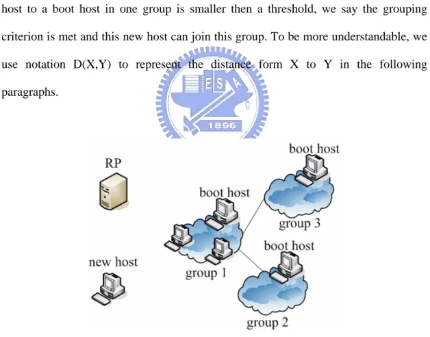
(13) Chapter 2 Super Node Selection Algorithm 2.1 Basic Concepts The principle of our algorithm is trying to partition all super nodes into many groups. Super nodes in the same group are considered close to each other. Each group has a boot host (the leader). When a user needs a super node, he can first make use of our algorithm to negotiate with the boot host and execute some measurements to find nearby group. Then, this user picks hosts in this group as super nodes. Because this super node is close to the user, thus, it can reduce the probability of inefficient routing mentioned in section 1.2. Before describing the algorithm, we need to introduce some terms used in our algorithm and the system architecture which is shown in Fig 2.1. Rendezvous Point (RP): RP is an entry point of a P2P network. Users which want to join a P2P network need to contact RP first in order to retrieve necessary information. Besides, RP maintains all super nodes data and structure information in our system. Super Node: A host can be a super node only if certain requirement is matched. In our IP communication platform, the function of a super node is used to relay media stream for those hosts behind NAT. So, the basic requirement of our super node is it must have a public IP address. RP will examine this requirement when a host contacts RP. In addition, we also take workload and computer power of a host into account. Boot host: A boot host is a leader in a group. It is responsible for replying the measuring request for searching a nearby super node from a new host. When a new 5.

(14) host attempts to apply our algorithm to search a nearby super node, it just negotiates with the boot host in this group. Group: A group is a set of hosts which are close to the boot host. A group acts as an end host. By utilizing this kind of hierarchical architecture can reduce communicating traffic and negotiation time. Neighbor Group: A neighbor group is a nearby group in the physical network. As shown in Fig 2.1, both group 2 and group 3 are the neighbor group of group 1. Grouping Criterion: Grouping criterion determines which group a new host should belong to. If the distance (the distance can be the round-trip time) from a new host to a boot host in one group is smaller then a threshold, we say the grouping criterion is met and this new host can join this group. To be more understandable, we use notation D(X,Y) to represent the distance form X to Y in the following paragraphs.. Fig 2.1 System architecture. 6.

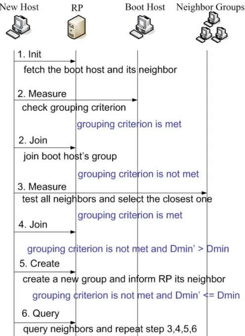
(15) 2.2 Select a Super Node In this section, we describe the detailed super node selection algorithm. We use a recursive algorithm to search the group close to the user. The pseudo code of our algorithm is shown as follows,. (bootHost, bootGroup) = fetchInformation(RP); while (true) { If(grouping criterion is met) { joinGroup(newHost, bootGroup); return; } else { Dmin = distance(newHost, bootHost); (minBootHost, minBootGroup) = measureClosestNeighbor(bootGroup); Dmin’ = distance(newHost, minBootHost); If(Dmin <= Dmin’) { newGroup = createGroup(newHost); addNeighborGroup(newGroup bootGroup); return; } Else { bootHost = minBootHost; bootGroup = minBootGroup; } } }. 7.

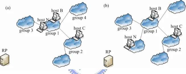
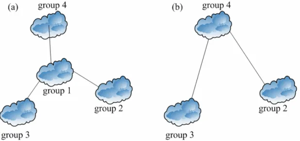
(16) When a new host wants to find nearby super nodes, it must contact RP to acquire necessary information. After RP receives the request of this new host, RP will randomly select a boot host for him. As illustrated in Fig 2.2-1, host N communicates to RP, than RP informs host N that the boot host is host B and host B is in group 1. Besides, RP also tells host N the neighbors of group 1 (group 2, group 3 and group 4) and each boot host in these neighbors.. Fig.2.2-1 Illustrate super node selection algorithm. After host N receives these information from RP, host N measures the distance from itself to the boot host. As illustrated in Fig 2.2-1, host N measures D(N, B). If the grouping criterion is met, it means host N is close to host B and host N can join group 1. Host N will notify RP it belongs to group 1 and our algorithm is finished. Finally, our system structure is shown in Fig 2.2-2 (a). If the grouping criterion is not met, host N will record D(N, B) and denote as Dmin. Dmin is the minimum distance and group 1 is the closest group up to now. Than, host N will sequentially measure the distance from itself to each boot host in host B’s neighbor groups. After completing these measurements, host N can determines the smallest distance and denotes as Dmin’. In this example, we assume 8.

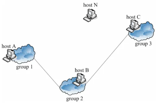
(17) D(N, C) is the smallest. If Dmin’ is greater than Dmin, it means Dmin is the best distance which our algorithm can find and our algorithm is finished. Host N will notify RP to create a new group for him and the group which holds Dmin will be chosen as its neighbor group. The new system structure is shown in Fig 2.2-2 (b). If Dmin’ is smaller then Dmin, host N will recursively repeat above paragraph to search the closest group.. Fig 2.2-2 Illustrate system architecture Those peers which don’t satisfy super node requirements can also follow the above procedure to find their super nodes. The difference is they only tell RP which group their preferred super nodes are located; they don’t need to join our system.. 2.3 Improvements Our algorithm would fail to find the closest group in the scenario shown in Fig 2.3-1. A new user, host N, attempts to find the closest super node. In this example, we assume D(N, A) is smaller than D(N, B) and group 3 is the closest group for host N. If RP choose host A in group 1 as the boot host and inform host N. By following our 9.

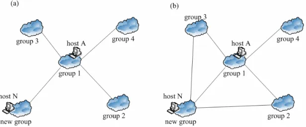
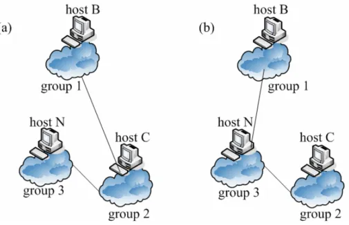
(18) algorithm, host N measures D(N, A) and it finds D(N,A) do not satisfy the grouping criterion. Next, host N will search the neighbor group of group 1. Then, host N finds the closest neighbor group is group2 but D(N, B) is greater than D(N, A). So, it will inform RP to create a new group and notify RP that group 1 is the neighbor group of this new group. In this scenario, host N do not have chance to measure the distance from itself to the boot host in group 3. Thus, host N can not find the super nodes in group 3.. Fig 2.3-1 Exception scenario. In order to have better performance, we present two methods to improve the drawback. First, RP gives the new host more boot hosts and the new host executes our algorithm from more boot hosts at the same time. By searching more hosts, it can increase the probability to search the closest super node. We evaluate the performance by giving the new host three boot hosts and five boot hosts. Second, a new group connects to more than one neighbor. Our structure will change from tree structure to graph structure. The effect of connecting more 10.

(19) neighbors is the same as above improvement. A new host will search more hosts and increase the probability to find the closest super node. Fig 2.3-2 illustrates the method to find more neighbors. As illustrated in Fig 2.3-2 (a), host N completes our algorithm and find group 1 is the closest group. We assume D(N, A) is not met the grouping criterion. Thus, host N will form a new group and select group 1 as its neighbor. Because of the locality characteristic, the neighbor groups of group 1 may be close to the new group. Therefore, host N can select more nearby neighbor groups from group 1’s neighbor groups. In Fig 2.3.2 (b), host N also connects to group 2 and group 3.. Fig 2.3-2 Change from tree structure to graph structure. The third improvement method is to select a boot host close to the new host. This can be done by checking IP address. We can select the boot host which has the same IP class as the new host. If we can give the new host a nearby boot host in the beginning, it can reduce many unnecessary measurements. In simulation, we first select the boot host with the distance from this boot host to the new host is smaller than a range. This range is greater than the threshold of the grouping criterion. If we can not find such boot hosts, we will randomly select a boot host from all boot hosts.. 11.

(20) 2.4 Fault Tolerant Model In order to prevent a communication being suspended due to the departure or failure of a super node, we present a scheme to relieve this problem. In addition to the super node for relaying media stream, a user can acquire a set of backup super nodes, hence a user can switch to another super node as it is aware of the serving super node is leaved. A super node may leave our system for any reason at any time. To detect the unpredictable departure of a super node, a super node is asked to periodically send out “keep alive” messages to the user it served. If a super node failed, the user can detect this phenomenon after a period of time as it didn’t receive “keep alive” message. Those super nodes which don’t serve anyone need another mechanism to detect the unpredictable departure. All hosts needs to maintain the same host list which includes all hosts in this group. When a new host decides to join a certain group, it would notify RP and the boot host in that group. After the boot host knows a new host joins this group, it will notify other hosts to update their host list. The boot host needs to periodically send out “keep alive” messages to other hosts in this group. When other hosts receive “keep alive” message, they will ack “keep alive” message in order to indicate their existence. If the second host in the host list didn’t receive “keep alive” message after a period of time, it will automatically become the boot host and notify RP the departure of the original boot host. Besides, the boot host also sends out “keep alive” messages to boot hosts in its neighbor groups. If there is only one host in a group, the departure of the boot host, the only one host, can be detected by the boot host in its neighbor groups. The reason for two kinds of mechanism is the previous mechanism requires more real-time reaction to the departure of a super node.. 12.

(21) Component. Information. RP. all super nodes information, system structure information. Super nodes. the information of hosts in the same group, the neighbor groups information, the neighbor boot hosts information. Normal users. which group he belongs to Table 2.4 The information stored in each component. 2.5 Restructure Architecture If all hosts in a group have leaved, that will result in an isolation of our structure. As can be seen from Fig 2.5 (a), if there is no host in group 1, our structure will separate into disconnected parts. Obviously the isolation will affect the functionality of our algorithm. To solve this problem, RP must notify the boot hosts in group 2 and group 3 of re-executing our algorithm and inform them the boot host is in group 4. After the boot hosts in group 2 and group 3 finished the algorithm in section 2.2, the final system structure is illustrated in Fig 2.5 (b).. Fig 2.5 Restructure architecture. 13.

(22) 2.6 Path Optimization Considering a situation in Fig. 2.6.1 (a), a new super node, host N, intends to join our system. The boot host of group1 is host B and the boot host of group 2 is host C. In this topology, we assume D(N, B) is greater than D(N, C) and both D(N, B) and D(N, C) are smaller then D(B, C). Both D(N, B) and D(N, C) do not meet grouping criterion. RP informs host N that the boot host is host B. By following our algorithm in section 2.2, host N will create a new group and choose group 2 as its neighbor group. If a boot host is far from the boot hosts in its neighbor group, it will increase the cost of fault tolerant model. Because both D(N, B) and D(N, C) are smaller then D(B, C), the time for sending KAM to its neighbor boot hosts in topology of Fig 2.6.1 (a) is greater than that in topology of Fig 2.6.1 (b). In order to achieve better performance, we should adjust the topology of Fig 2.6.1 (a) to the topology of Fig 2.6.1 (b). D(B, C) has been measured when host B or host C joined our system. D(N, B) and D(N, C) are measured when host N intends to join our system. Therefore, by comparing these data, we can know the relation between group 1, group 2 and group 3 and modify our structure to Fig 2.6.1 (b).. 14.

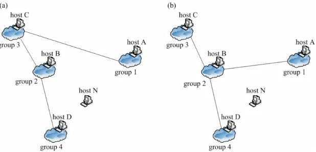
(23) Fig 2.6.1 Path optimization. The effect of path optimization is either good or bad to our super node selection algorithm. As shown in Fig 2.6.2, path optimization will help the new host to find the closest group. Assuming the distance relationship in Fig 2.6.2 is D(N, C)>D(N, A)>D(N, B)>D(N, D) and D(N, C), D(N, A), D(N, B) and D(N, D) do not satisfy the grouping criterion. After the new host N contacts RP to retrieve the information of the boot host. RP informs the new host N that the boot host is host A and host A is in group 1. In Fig 2.6.2 (a), we do not perform path optimization for host B. By following our algorithm, host N measures D(N, A) and knows D(N, A) do not meet the grouping criterion. Then host N searches the neighbor group of group 1. He also finds D(N, C) do not meet the group criterion and D(N, C) is greater than D(N, A). Host N will create a new group and choose group 1 as its neighbor group. In Fig 2.6.2 (b), we perform path optimization for host B. By following our algorithm, host N has the chance to measure host B and host D. Thus, host N can find the closest group is group 4.. 15.

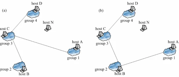
(24) Fig 2.6.2 Path optimization may increases performance. As shown in Fig 2.6.3, the effect path optimization will make the new host hard to find the closest group. Assuming the distance relationship in Fig 2.6.3 is D(N, B)>D(N, A)>D(N, C)>D(N, D) and D(N, B), D(N, A), D(N, C) and D(N, D) do not satisfy the grouping criterion. After the new host N contacts RP to retrieve the information of the boot host. RP informs the new host N that the boot host is host A and host A is in group 1. In Fig 2.6.3 (a), we do not perform path optimization for host B. By following our algorithm, host N has the chance to measure host C and host D. Thus, host N can find the closest group is group 4. In Fig 2.6.3 (b), we perform path optimization for host B. By following our algorithm, host N measures D(N, A) and knows D(N, A) do not meet the grouping criterion. Then host N searches the neighbor group of group 1. He also finds D(N, B) do not meet the group criterion and D(N, B) is greater than D(N, A). Host N will create a new group and choose group 1 as its neighbor group.. 16.

(25) Fig 2.6.3 Path optimization may decreases performance. 2.7 Reduce Overhead of Querying Neighbors This problem is a new host need to contact RP to fetch neighbors’ information when it wants to perform next measurement. If this new host is far from RP, this will increase cost of our algorithm. To be more clearly, the negotiation flow can be shown as Fig 2.7. To overcome this disadvantage, the boot host needs to store its neighbors’ information. When a new host creates a new group and notifies RP its neighbor group, RP also informs the boot host in its neighbor group to update neighbor’s information. While a boot host receives a measure request from a new host, the boot host will reply the neighbors’ information to the new host.. 17.

(26) Fig 2.7 Negotiation Flow for completing selecting algorithm. 18.

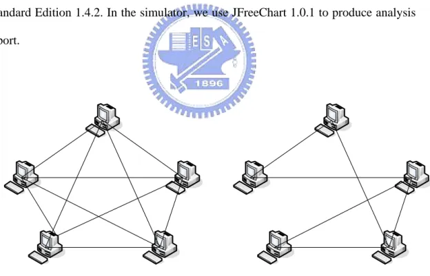
(27) Chapter 3 Simulation and Analysis In the following sections, we carry out a simulation to verify the results and quantify the performance of our algorithm.. 3.1 Implementation of the Simulator We have implemented a simulator on Microsoft Windows Platform and our developing tool is Borland JBuilder 2005. The language version is Java(TM) 2 SDK, Standard Edition 1.4.2. In the simulator, we use JFreeChart 1.0.1 to produce analysis report.. Fig 3.1 (a) Random topology (b) Waxman topology. We use two kind of network topology as our experimental environment. The first network topology is shown in Fig 3.1 (a). We randomly generate hosts on a plane and. 19.

(28) the distance between two hosts is this distance on this plane. In the following paragraphs, we use Random topology to stand for this topology. The second network topology is shown in Fig 3.1 (b) and it is generated by BRITE [13]. BRITE is a widely-used network topology generator and it is used in many famous network simulation tools such as ns and SSF. There are several kinds of topology mode in BRITE and we use Waxman [14] model to generate network topology. Waxman model produces a random graph on a plane, but it includes network specific characteristics and it uses a probability function to connect two nodes. The distance between two hosts which do not have direct connection is calculated by Dijkstra shortest path algorithm. The configuration file we used for setting Waxman model is shown in Table 3.1. The number of nodes (N) and the size of main plane (HS) are assigned for different simulation.. BeginModel Name = 3 #Router Waxman = 1, AS Waxman = 3 N=X #Number of nodes in graph HS = Y #Size of main plane (number of squares) LS = 100 #Size of inner planes (number of squares) NodePlacement = 1 #Random = 1, Heavy Tailed = 2 GrowthType = 1 #Incremental = 1, All = 2 m=2 #Number of neighboring node each new node connects to. alpha = 0.15 #Waxman Parameter beta = 0.2 #Waxman Parameter BWDist = 1 #Constant = 1, Uniform = 2, HeavyTailed = 3, Exponential = 4 BWMin = 10.0 BWMax = 1024.0 EndModel. Table 3.1 Waxman model parameters. 20.

(29) 3.2 Simulation Results and Analysis We first present the topology produced by our simulator. Then, we discuss the analysis reports about randomly selecting a boot host and two improvements.. 3.2.1 Simulation Results. The system structure produced by our algorithm can be seen in Fig 3.2.1. There are 100 hosts in Fig 3.2.1. Each circle stands for a host and only the boot host has edges to connect neighbor groups.. Fig 3.2.1 System structure 21.

(30) 3.2.2 Simulation Analysis. We evaluate our algorithm by the following two terms. Join Cost is used to calculate the number of hosts are measured after a new host completes our algorithm. Performance is used to determine whether the super node selected by our algorithm is the closest one or not. Join Cost =. the number of hosts are measured after a host (A) completes our algorithm x100% the number of hosts in our system when A executes our algorithm. Performance =. the rank of distance from a host (A) to a group selected by our algorithm x100% the number of groups in our system when A executes our algorithm. Fig 3.2-1 is performed in first topology with 100 nodes. Fig 3.2-2 is performed in second topology with 100 nodes. Both analyses show that our algorithm can not find the closest group. Because we do not explore all nodes, we can not ensure that there are no other super nodes are closer than the super node we selected. Table 3.2.2-1 is the distribution of the performance. Only 37% nodes can find the closest group in Random topology and 32% nodes find the closest group in Waxman topology.. Fig 3.2.2-1 100 nodes and 1 boot host in Random topology. 22.

(31) Fig 3.2.2-2 100 nodes and 1 boot host in Waxman topology. Table 3.2.2-1 Performance results with 100 nodes and 1 boot host Num of Nodes Random Topology Performance. Waxman Topology. < 80%. 21. 25. 80%~89%. 10. 21. 90%~99%. 32. 22. 100%. 37. 32. Fig 3.2-3 is performed in first topology with 100 nodes and three boot hosts. Fig 3.2-4 is performed in first topology with 100 nodes and five boot hosts. As can be seen from Fig 3.2-3 and Fig 3.2-4, given three boot hosts can achieve better balance between performance and the cost of selecting a super node. Giving more boot hosts can’t improve the performance significantly but increasing more traffic.. 23.

(32) Fig 3.2.2-3 100 nodes and 3 boot hosts in Random topology. Fig 3.2.2-4 100 nodes and 5 boot hosts in Random topology. Table 3.2.2-2 Performance results with multi boot hosts in Random topology Num of Nodes Performance. 3 boot hosts. 5 boot hosts. < 80%. 2. 1. 80%~89%. 7. 3. 90%~99%. 24. 16. 100%. 67. 80. 24.

(33) Fig 3.2-5 is performed under Waxman topology with 100 nodes and three boot hosts. Fig 3.2-6 is performed under Waxman topology with 100 nodes and five boot hosts. Both analyses show the first improvement method also works in Waxman topology.. Fig 3.2.2-5 100 nodes and 3 boot hosts in Waxman topology. Fig 3.2.2-6 100 nodes and 5 boot hosts in Waxman topology. 25.

(34) Table 3.2.2-3 Performance results with multi boot hosts in Waxman topology Num of Nodes Performance. 3 boot hosts. 5 boot hosts. < 80%. 1. 0. 80%~89%. 3. 1. 90%~99%. 33. 11. 100%. 63. 88. Fig 3.2-7 and Fig 3.2-8 are evaluated under Random topology and Waxman topology with 100 nodes and one boot host. Both simulations adopt the second improvement method. These two analyses show the second improvement can greatly enhance the performance even if there is only one boot host.. Fig 3.2.2-7 100 nodes and 1 boot host in Random topology. 26.

(35) Fig 3.2.2-8 100 nodes and 1 boot host in Waxman topology. Table 3.2.2-4 Performance results with locality selection Num of Nodes Performance. Random Topology. Waxman Topology. < 80%. 0. 3. 80%~89%. 0. 2. 90%~99%. 18. 16. 100%. 82. 79. Following analyses are evaluated with 500 nodes. Fig 3.2-9 is performed in Random topology with 500 nodes and three boot hosts. Fig 3.2-10 adopts the second improvement and is performed in Random topology with 500 nodes and one boot host. These results show that our algorithm works well and do not cost too much network traffic when network topology grows due to the characteristic of the tree structure.. 27.

(36) Fig 3.2.2-9 500 nodes and 3 boot host in Random topology. Fig 3.2.2-10 500 nodes and 1 boot host in Random topology Table 3.2.2-5 Performance results with 500 nodes in Random topology Num of Nodes Performance. 3 boot hosts Random selection. 1 boot host Locality selection. < 80%. 36. 2. 80%~89%. 55. 0. 90%~99%. 273. 152. 100%. 136. 346. 28.

(37) Fig 3.2-11 is performed under Waxman topology with 500 nodes and three boot hosts. Fig 3.2-12 adopts the second improvement and is evaluated under Waxman topology with 500 nodes and two boot hosts. Our algorithm also works well in Waxman topology and do not cost too much network traffic when network topology grows.. Fig 3.2.2-11 500 nodes and 3 boot hosts in Waxman topology. Fig 3.2.2-12 500 nodes and 2 boot hosts in Waxman topology. 29.

(38) Table 3.2.2-6 Performance results with 500 nodes in Waxman topology Num of Nodes Performance. 3 boot hosts Random selection. 1 boot host Locality selection. < 80%. 9. 13. 80%~89%. 23. 33. 90%~99%. 293. 109. 100%. 175. 345. Following tables are the comparison of the effect of path optimization and the effect of the graph structure. The analyses are average results of 100 simulations. As can be seen from Table 3.2.2-7, path optimization can slightly increase the performance of our algorithm. The graph structure would increase a little join cost and slightly enhance the performance. Table 3.3.3-8 is evaluated in Waxman topology. The effect of path optimization and graph structure is the same as Table 3.2.2-7.. Table 3.2.2-7 Comparison of path optimization and graph structure in Random topology Num of Nodes. Path Optimization. Without Path Optimization. Path Optimization Graph. < 80%. 21.46. 25.23. 16.39. 80%~89%. 13.28. 13.64. 10.91. 90%~99%. 29.75. 28.61. 30.28. 100%. 35.51. 32.52. 42.42. Average %. 87.19. 84.78. 89.36. Average Join Cost. 5.5. 5.3. 5.8. Performance. 30.

(39) Table 3.2.2-8 Comparison of path optimization and graph structure in Waxman topology Num of Nodes. Path Optimization. Without Path Optimization. Path Optimization Graph. < 80%. 23.97. 25.14. 21.81. 80%~89%. 13.36. 17.51. 11.65. 90%~99%. 30.4. 30.39. 29.87. 100%. 32.27. 26.96. 36.67. Average %. 86.61. 85.3. 87.42. Average Join Cost. 6.1. 5.7. 7.2. Performance. 31.

(40) Chapter 4 Conclusions In this thesis, we present an algorithm to overcome the disadvantages of selecting a super node without taking locality into consideration. In order to prevent selecting a super node that is far from both communicating pairs, we try to find a super node close to one of them. We adopt a greedy algorithm to search such super nodes. Computer simulation has also been conducted to evaluate our algorithm. The simulation results indicate this greedy algorithm can not obtain the closest super node. To improve the performance, we present three approaches and these approaches indeed work in simulation result. First, giving more boot hosts to the new host. By searching more hosts, it can increase the probability to find the closest group. Experimental result reveals that given three boot hosts can achieve acceptable balance between the performance and the cost of selecting a super node. Second, a new group can connect to more than one group. The graph structure also increases the number of searched hosts. Third, RP selects a boot host close to the new host. This can be done by checking IP address. Experimental result shows that the second approach can significantly enhance the performance and reduce the cost of selecting a super node. Because we adopt a P2P-like solution to choose peers with high capacity as super nodes, we have to select super nodes from a large number of hosts and dynamically changing network. In order to prevent exploring all networks and reduce network traffic, we use a hierarchy structure and partition super nodes into groups by measuring the transmission delay. Furthermore, we also present a mechanism relieve the problem due to the unpredictable departure of a super node. The future work is to ensure each node in the same group is close to each other. In order to reduce network traffic, we only measure the distance from a host to a boot. 32.

(41) host. As a result, each node in the same group is only close to the boot host. If the current boot host leaves, nodes in the same group may not be close to the next boot host. In order to achieve this requirement, the new host may measure more hosts in one group.. 33.

(42) Reference [1] Jian Liang, Rakesh Kumar and Keith W. Ross, “The KaZaA Overlay: A Measurement Study”, September 15 2004. [2] Salman A. Baset and Henning Schulzrinne, “An Analysis of the Skype Peer-to-Peer Internel Telephony Protocol”, September 2004. [3] Gnutella Protocol Specification. http://www.the-gdf.org/ [4] Virginia Lo, Dayi Zhou, Yuhong Liu, Chris GauthierDickey, and Jun Li, “Scalable Supernode Selection in Peer-to-Peer Overlay Networks”, IEEE Proceedings of the 2005 Second International Workshop on Hot Topics in Peer-to-Peer Systems, 2005. [5] S. Ratnasamy, P. Francis, M. Handley, R. Karp, and S. Shenker, “A scalable content-addressable network,” presented at the ACM SIGCOMM, San Diego, CA, Aug. 2001. [6] A. Rowstron and P. Druschel, “Pastry: Scalable, distributed object location and routing for large-scale peer-to-peer systems,” presented at the 18th IFIP/ACM Int. Conf. Distributed Systems Platforms (Middleware 2001), Heidelberg, Germany, Nov. 2001. [7] Honghao Wang, Yingwu Zhu and Yiming Hu, “An Efficient and Secure Peer-to-Peer Overlay Network”, IEEE Symposium on Applications and the Internet, 2003. [8] K. Egevang, P. Francis, “The IP Network Address Translator (NAT)”, RFC 1631, May 1994. [9] J. Rosenberg, J. Weinberger, C. Huitema and R. Mahy, ”STUN-Simple Traversal of User Datagram Protocol (UDP) Through Network Address Translators (NATs)”, RFC 3489, March 2003.. 34.

(43) [10] Kazaa Website. http://www.kazaa.com [11] Skype Website. http://www.skype.com/ [12] J. Rosenberg, Henning Schulzrinne, G. Gamarillo, E. Schooler, Mark Handley, A. Johnston, J. Peterson, R. Sparks, M. Handley, “SIP: Session Initiation Protocol”, RFC 3261, IETF, June 2002 [13] BRITE: Boston University Representative Internet Topology Generator. http://www.cs.bu.edu/brite/index.html. [14] B. M. Waxman, “Routing of Multipoint Connections”, IEEE Journal on Selected Areas in Communications. VOL.6. NO.9. Dec. 1988.. 35.

(44)