針對掃描式蠕蟲做準確偵測之適應性接續假設測試

國 立 交 通 大 學

電 信 工 程 學 系 碩 士 班

碩 士 論 文

針對掃描式蠕蟲做準確偵測之

適應性接續假設測試

Adaptive Sequential Hypothesis Testing for Accurate

Detection of Scanning Worms

研究生：李松晏

指導教授：李程輝 教授

針對掃描式蠕蟲做準確偵測之適應性接續假設測試

Adaptive Sequential Hypothesis Testing for Accurate Detection of

Scanning Worms

 

研究生：李松晏 Student: Sung-Yen Lee

指導教授：李程輝 教授 Advisor: Prof. Tsern-Huei Lee

       

國 立 交 通 大 學

電 信 工 程 學 系 碩 士 班

碩 士 論 文

        A Thesis

Submitted to Institute of Communication Engineering Collage of Electrical Engineering and Computer Science

National Chiao Tung University in Partial Fulfillment of Requirements

for the Degree of Master of Science

in

Communication Engineering June 2009

Hsinchu, Taiwan, Republic of China  

針對掃描式蠕蟲做準確偵測之

適應性接續假設測試

學生：李松晏 指導教授：李程輝 教授 國立交通大學 電信工程學系碩士班 中文摘要 早期偵測掃描式蠕蟲的技術，是建立在惡意行為的主機具有較高掃描率的基 礎上。此種方法對於秘密的掃描並不適用，且一旦發出警告的掃描率門檻被攻擊 者所知悉，便能輕易躲過這種偵測。為了克服這樣的問題，「接續假設測試」便 成為一種替代方案。這種方法所需要觀測連線嘗試結果的次數較少，從這個角度 看來，它比起基於掃描率的方法，可以更快偵測出掃描式蠕蟲。然而，接續假設 測試的方法，對於正常主機與惡意行為主機的第一次連線嘗試的成功機率相當敏 感。如果事前不知道此機率，誤判率可能會比理想值高出許多。在這篇論文中， 我們提出一個簡單的適應性演算法，可以準確地估計出這些機率。實驗結果顯 示，我們提出的適應性估計演算法，對於原本的接續假設性測試法有很大的改 善，因為它使原本對於偵測掃描式蠕蟲的方法更加健全完善。

Adaptive Sequential Hypothesis Testing for Accurate

Detection of Scanning Worms

Student: Sung-Yen Lee Advisor: Prof. Tsern-Huei Lee

Institute of Communication Engineering National Chiao Tung University

Abstract

Early detction techniques of scaning worms are based on simple observations of high port/address scanning rates of malicious hosts. Such apporaches are not able to detect stealthy scanners and can be easily evaded once the threshold of scanning rate for generating alerts is known to the attackers. To overcome this problem, sequential hypothesis testing was developed as an alternative detection technique. It was found that the technique based on sequential hypothesis testing can detect scanning worms faster than those based on scanning rates in the sense that it needs fewer observations for the outcomes of connection attempts. However, the performance of the detection technique based on sequential hypothesis testing is sensitve to the probabilities of success for the first-contact connection attempts sent by benign and malicious hosts. The false positive and false negative probabilities could be much larger than the desired values if these probabilities are not known. In this paper, we presnt a simple adpative algorithm which provides accurate estimates of these probabilities. Numerical results show that the proposed adaptive estimation algorithm is an important enhancement of sequential hypothesis testing because it makes the technique robust for detection of scanning worms.

誌謝

感謝我的指導教授─李程輝老師，在研究所的求學過程中悉心地指導我。您無比的 研究熱忱和適時給予我的鼓勵，讓我對研究產生了興趣和信心。在您的教誨下，我學習 到了做研究應有的態度與嚴謹的思維，在做研究和撰寫論文的過程，我得到了許多保貴 的經驗，實在是獲益匪淺。平時您的親和力和幽默感，更拉近了師生間的距離，讓實驗 室的氣氛既溫暖又歡樂。 感謝 NTL 實驗室整個大家庭的成員。景融學長和迺倫學姐，很幸運能坐在你們旁 邊，你們不只給予我研究和課業的指導，更時常關心照顧我、陪我聊天，還有文生哥、 瑋哥、阿成哥、庚哥、鑫哥、YY、西西搭、北極、世弘和凱文，眾位學長對我的照顧， 我都感念在心；感謝同窗的大頭、丹奇、鈞傑、佑信、逼恩、堯堯和小汪，這些日子除 了和你們一起修課、做研究，還常常一起打球、聚餐、打嘴砲，讓我過得很快樂；謝謝 呷菜、韋儒、小机、小薇、熊仔、阿倫這群可愛的學弟妹，你們讓實驗室變得更活潑熱 鬧有朝氣。這兩年來跟大家朝夕相處，讓我的碩士生涯過得很充實愉快，充滿了各種美 好的回憶。 最後，更要特別感謝我的父親李森乾先生與母親王美純女士，謝謝您們對我從小無 微不至的養育照顧與支持，讓我無後顧之憂地完成學業。感謝我的兄長李京螢先生，謝 謝您平時對我的關心和勉勵。因為您們，才能讓我求學之路走得如此堅定踏實！ 謹將此論文獻給所有愛我與我愛的人 2009 年 6 月 於風城交大

Contents

中文摘要 ... i Abstract ... ii 誌謝 ... iii Chapter 1. Introduction ... 1 Chapter 2. Background ... 6 2.1 Scanning worms ... 6

2.2 Type I and type II errors ... 8

Chapter 3. Related Works ... 11

Chapter 4. Adaptive Sequential Hypothesis Testing ... 17

Chapter 5. Experimental Results ... 21

Chapter 6. Conclusion ... 27

List of Tables

Table 1: Definition of false positive and false negative ... 9

Table 2: Example of false positive and false negative ... 9

Table 3: Data structure of the adaptive sequential hypothesis testing algorithm. ... 18

Table 4: Data structure for updating θ and ˆ_{0 θ . ... 19} ˆ₁

Table 5: Estimates of θ₀ and θ_{1 for the proposed adaptive algorithm. ... 24}

Table 6: The average number of FCC requests to detect a remote host as benign. ... 25

List of Figures

Figure 1: Comparison of false positive probabilities. ... 23 

Chapter 1.

Introduction

The rapid advances of computer and network technologies allow modern

computer worms to spread at a speed much faster than human-mediated responses.

The Code Red [6], Nimda [7], and Slammer [8] that were detected in recent years

infected hundreds of thousands of computers on the Internet in a very short period

of time and caused huge economic loss to our society. Fast and accurate

detection of worms as they are spreading is, therefore, very important to prevent

the majority of vulnerable systems from being infected and minimize the damage.

Current computer worm detection technologies can be classified into three

categories, namely, protocol analysis, pattern matching, and behavior anomaly.

Protocol analysis is a technique which examines the header of a packet to ensure

there is no misuse of protocol fields. For example, the OID field of an SNMP

packet should be a certain number of bytes. There is something wrong (say, an

overflow attack) if the next expected field does not appear after this number of

payload of a packet or across packets. A specific unique pattern or string of

malicious codes can be extracted as the signature of a worm and be used in the

detection process. Although pattern matching is accurate, it is limited to known

worms with identified signatures. The majority of vulnerable systems could be

infected if the signature of a new worm is not created quickly. Finally, behavior

anomaly can be used to detect and prevent the outbreak of an attack because an

infected host is likely to behave differently from a normal host. As an example, a

host infected by some scanning worm may try to infect other vulnerable hosts on

the Internet with port/address scanning. Therefore, one can detect an infected

host with the observation of high new connection attempt rate or high failure ratio

of first-contact connection attempts [1]. Worm detection based on behavior

anomaly is receiving more and more attention because it can detect the so-called

“zero-day” attacks and polymorphous worms without signatures.

Early behavior anomaly based scanning worm detection techniques were

designed according to simple observations of high scanning rate by an infected

host. For example, the criterion used in the Network Security Monitor (NSM) [5]

is to detect any source IP address which connects to more than M distinct

rules. It detects a source IP address which sends connection attempts to more

than U number of ports or V number of IP addresses within S seconds. An

obvious drawback of such approaches is that an attacker can easily evade

detection once the parameter values are known.

The authors of [1] observed from real traces that the failure probability of a

connection attempt sent by an infected or malicious host is much higher than that

of a connection attempt sent by a benign host. As a result, the technique of

sequential hypothesis testing was developed for scanning worm detection. Their

algorithm is called Threshold Random Walk (TRW). A failed (or successful)

connection attempt causes the random walk to move upward (respectively,

downward). A host is declared as malicious if the position of its corresponding

random walk is greater than the upper threshold or as benign if it is smaller than

the lower threshold. The step size of moving upward could be different from the

step size of moving downward. Compared with previous detection techniques,

the TRW algorithm is able to detect stealthy scanning and the detection process is

fast in the sense that it need only observe a few connection attempts. A

simplified algorithm which is suitable for both software and hardware

moving upward and downward are identical. The reversed sequential hypothesis

testing presented in [2] can detect malicious scanners faster than the TRW

algorithm. However, it slightly increases the false positive probability. The

TRW algorithm, its simplified version, and the reverse sequential hypothesis

testing will be reviewed in Chapter 3.

A fundamental assumption of the TRW algorithm is that the success

probabilities of connection attempts sent by malicious and benign hosts are

known. These probabilities are used to compute the step sizes of moving upward

and downward. Unfortunately, this assumption may not be valid in a real system.

In this paper, we investigate the effect of using estimated probabilities to the false

positive and the false negative probabilities. Results show that the performance

of the TRW algorithm is sensitive to the estimated probabilities. The false

positive and false negative probabilities could be significantly larger than the

desired values if inaccurate estimates are used. In order to make TRW works

properly, we develop an adaptive algorithm which estimates the success

probabilities of connection attempts based on their outcomes. According to

simulation results, our proposed adaptive algorithm provides estimates of success

negative probabilities are also close to the desired values.

The rest of this paper is organized as follows. In Chapter 2, we introduce

some background about scanning worms and type I and type II errors. In

Chapter 3, we review the TRW algorithm, its simplified version, and the reversed

sequential hypothesis testing. In Chapter 4, we present our proposed adaptive

algorithm for estimation of success probabilities of connection attempts.

Experimental results are provided in Chapter 5. Finally, we draw conclusion in

Chapter 2.

Background

2.1 Scanning worms

Computer worms are malicious software applications designed to spread via

computer networks without human intervention. Scanning worms locate

vulnerable hosts by generating a list of addresses to probe and then contact them.

They can self-propagate among the hosts exploiting security or policy flaws in

widely-used services [11]. An infected host initiates scans and infects the other

benign hosts. Subsequently, the benign hosts may be infected and then join the

army of scanning. Finally, more and more hosts on the Internet will be infected.

The list of addresses can be generated sequentially or pseudo-randomly.

Local addresses are often preferentially selected because the communication

between neighboring hosts will likely encounter fewer defenses [12]. Scans

may take the form of TCP connection requests (SYN packets) or UDP packets.

packet to also contain the body of the worm, such as the Slammer worms [8].

Scanning worms probe attempts to determine if a service is operating at a

target IP address and then discover new victims. They have two basic scanning

types – horizontal scans and vertical scans. The former look for an identical

service on a large number of hosts, and the latter examine an individual host to

discover all running services.

There are many kinds of techniques to generate a list of addresses for

scanning worms, such as linear scanning of an IP address space (Blaster), fully

random (Code Red), a bias toward local address (Code Red II and Nimda), or

even more enhanced techniques (Permutation Scanning). While more and more

scanning worms change their style of scanning to avoid being detected, all of

them still have two common properties as follows. Most of the scanning

attempts may result in failure, and the infected hosts will send many connection attempts [3]. As long as we look for a class of behavior rather than specific

2.2 Type I and type II errors

In statistics, the terms Type I error (α error, or false positive) and type II error

(β error, or a false negative) are used to describe possible errors made in a

statistical decision process.

Type I error: the error of rejecting a null hypothesis when it is actually true. Plainly speaking, it occurs when we are observing a difference when in truth there

is none.

Type II error: the error of failing to reject a null hypothesis when it is in fact not true. In other words, this is the error of failing to observe a difference when in

truth there is one.

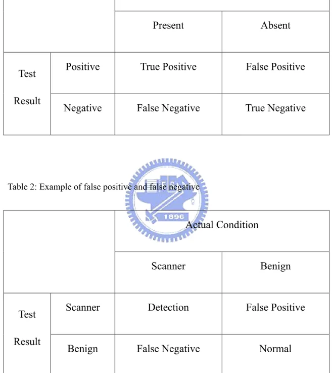
Table 1 illustrates the ambiguity, which is one of the dangers of this wider use:

They assume the speaker is testing for guilt; they could also be used in reverse, as

testing for innocence; or two tests could be involved, one for guilt, the other for

Table 1: Definition of false positive and false negative

Actual Condition

Present Absent

Test

Result

Positive True Positive False Positive

Negative False Negative True Negative

Table 2: Example of false positive and false negative

Actual Condition

Scanner Benign

Test

Result

Scanner Detection False Positive

When a host is determined to be malicious or benign, it’s possible to make an

error, such as regarding a benign host as malicious one or regarding a malicious

host as benign one. We hope that the scan detection mechanism can distinguish

between malicious and benign hosts as precisely as possible. In other words, we

hope the probability of false positive and false negative is as less as possible.

In this paper, we use the false positive probability and false negative probability

Chapter 3.

Related Works

In the TRW algorithm, an event is generated and monitored when a remote

source r makes a first-contact connection (FCC) request to a local destination l.

An FCC request is a connection request which is addressed to a host the sender

has not previously communicated. For simplicity, only TCP connections are

considered and thus a TCP SYN packet indicates a connection request. The

outcome of an FCC request is classified as either a “success” or a “failure”. It is

a success if host l replies a SYN-ACK packet or a failure if host l replies a RST

packet or does not reply at all. When extended to UDP connections, the first

UDP packet from r to l can be used to indicate a connection request and any UDP

packet from l to r before timeout can be considered as successful establishment of

For a given remote host r, let X_i be a random variable that represents the

outcome of the FCC request from r to the

_i

th _{distinct local host}

i

l , where

0 if the FCC request is a success =

1 if the FCC request is a failure

i

X ⎧⎪_⎨

⎪⎩

The outcomes of X₁, X₂, …, are observed so that host r can be determined

to be either malicious or benign. There are two hypotheses: H₀ and H₁, where

0

H is the null hypothesis that the remote host r is benign and H₁ is the

hypothesis that r is malicious. To simplify the analysis, it is assumed that, conditioning on hypothesis H_j, the random variables X H₁| _j, X₂|H_j, … are

independent and identically distributed (i.i.d.) with probability mass function

0 0 1 1 P 0 | P 0 | i i X H X H θ θ ⎡ ⎤ ⎣ ⎦ ⎡ ⎤ ⎣ ⎦ = = = = 0 0 1 1 P 1| 1 P 1| 1 i i X H X H θ θ ⎡ ⎤ ⎣ ⎦ ⎡ ⎤ ⎣ ⎦ = = − = = −

for some

θ

₀ and

θ

₁ which satisfy

θ θ

₀ > . ₁

Given the two hypotheses, there are four possible decisions. The decision is

called a detection if the algorithm selects H₁ when H₁ is true. On the other

hand, it is called a false negative if the algorithm chooses H₀ when H₁ is true.

selecting H₀ is called a normal. These four possible outcomes are represented as： 1 1 0 1 1 0 0 0 : P choose H | H is true : P choose H | H is true 1 : P choose H | H is true : P choose H | H is true 1 DT FN DT FP NM FP Detection P False Negative P P False Positive P Normal P P ⎡ ⎤ ⎣ ⎦ ⎡ ⎤ ⎣ ⎦ ⎡ ⎤ ⎣ ⎦ ⎡ ⎤ ⎣ ⎦ = = = − = = = −

The desired performance of the TRW algorithm can be specified with the detection probability P_DT and the false positive probability P_FP. Let

α

represent the upper bound of false positive probability and

β

denote the lower

bound of detection probability. In other words, we desire

and

FP DT

P ≤

α

P ≥

β

where typical values might be

α

=

0.01 and

β

=

0.99

.

As the outcome of X_i is observed, we calculate the likelihood ratio:

( )

n 1 1 n 1 n 0 0 P | H P | H P | H P | H n i i i X X = ⎡ ⎤ ⎡ ⎤ ⎣ ⎦ ⎣ ⎦ ⎡ ⎤ ⎡ ⎤ ⎣ ⎦ ⎣ ⎦ Λ X ≡ X =

∏

X

Note that (Λ Xn) can be updated incrementally. Let φ

( )

Xi represent the likelihood ratio of the

_i

th _{observation. It holds that}

( )

( )

(

n-1

)

( )

1 n n i i X X

φ

φ

= Λ X_n =

∏

=Λ X , Λ

( )

X₀ =1

The updated likelihood ratio (Λ Xn) is compared with an upper threshold

η

1

and a lower threshold

η

₀. If Λ

( )

X_n ≥η₁, then hypothesis H₁ is accepted. If

( )

η0

Λ X_n ≤ , then hypothesis H is accepted. More observations are needed if ₀

( )

0 1

η < Λ X_n <η .

It can be shown that

η

₁≤P_DT /P_FP and η₀ ≥ −

(

1 P_DT

)(

1−P_FP

)

[9]. In real

implementations, one can use the approximations P_FP = ,

α

P_DT = and set

β

1

η β α

= and η₀ = −

(

1 β

) (

1−α

)

. Moreover, the log-likelihood ratio can be used to simplify computation.

The huge complexity of monitoring FCC requests of all remote hosts makes the TRW algorithm infeasible. In [3], a simplified version which uses one bit to indicate whether or not host r has sent any packet to host l and another bit for the opposite direction for a given connection that is determined by the remote IP address, local IP address, source port, destination port, and protocol ID. A hash

negative probability is slightly increased. The step sizes of moving upward and downward are both set to one in the simplified version.

It is possible that a remote host is infected when its likelihood ratio is close to

but larger than

η

₀. In this case, it needs more observations for the TRW

algorithm to declare the host to be malicious than doing so for a host who is infected when its likelihood ratio is equal to 1. The reversed sequential

hypothesis testing proposed in [2] computes the likelihood ratio for the reversed vector of outcomes X_n =

(

X , , _n " X₁

)

observed so far. For this algorithm, the

likelihood ratio can be easily updated according to

( )

max

(

1, X

(

−1

)

φ

( )

n

)

Λ X_n = Λ X_n with Λ

( )

X₀ ≡1. It can detect malicious hosts

slightly faster than the TRW algorithm. However, it increases the false negative probability and does not detect benign hosts.

As mentioned before, the TRW algorithm assumes that

θ

₀ and

θ

₁ are

known, which may not be true in a real network. According to the numerical results to be presented in Chapter 5, the false positive and false negative

probabilities of the TRW algorithm could be much larger than the desired values if the adopted

θ

₀ and

θ

₁ are different from their true values. To overcome this problem, we propose in the next chapter an adaptive algorithm to estimate the

Chapter 4.

Adaptive Sequential Hypothesis Testing

Our proposed adaptive sequential hypothesis testing provides estimates of

0

θ

and

θ

₁ adaptively based on observations of the outcomes of FCC requests.

We will consider only the estimation procedure of

θ

₀. The estimation procedure

for

θ

₁ is similar.

The basic idea of our proposed estimation procedure is as follows. An

estimate of

θ

₀, denoted by θ , is generated when the total number of remote ˆ₀

hosts that are detected as benign is greater than or equal to K, where K is a design

parameter. Let S_i and F_i represent, respectively, the numbers of successful

and failed FCC requests sent by r_i when it is detected as benign. Furthermore,

let N_i = + . The estimate of S_i F_i

θ

₀ is given by ˆ₀

i i i i S N

θ

=

∑

∑

, for all i such that ri

is detected as benign.

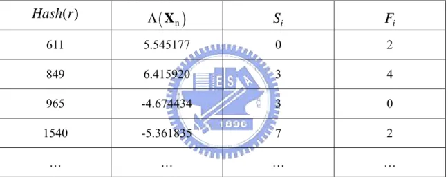
In the beginning, we need a data structure as shown in Table 3. When a

updated according to the outcome, i.e., success or fail, of the FCC. If the FCC request is classified as success, _{S of i} Hash r( ) is increased by one, where

( )

Hash r represents the hash result of IP address r. On the contrary, if the FCC

request is classified as fail, F_{i of ( )}Hash r is increased by one.

Table 3: Data structure of the adaptive sequential hypothesis testing algorithm. ( ) Hash r

( )

n Λ X S_i F_i 611 5.545177 0 2 849 6.415920 3 4 965 -4.674434 3 0 1540 -5.361835 7 2 … … … …

The remote host r is detected as benign if its likelihood ratio is lower than threshold

η

₀. On the other hand, if its likelihood ratio is higher than threshold

1

η

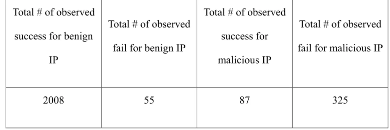
, the remote host r is declared as malicious. Once remote host r is decided as benign or malicious, the corresponding S_{i and} F_i values are added to the data

Table 4: Data structure for updating θ and ˆ_{0 θ .} ˆ₁

Total # of observed success for benign

IP

Total # of observed fail for benign IP

Total # of observed success for malicious IP

Total # of observed fail for malicious IP

2008 55 87 325

The estimates of

θ

₀ and

θ

₁ are obtained from Table 2. Initially, we set

0

ˆ _0.55

θ = and θˆ₁ =0.45. Note that choosing a small value for θˆ₀ and a large

value for θˆ₁ (as we did here) require more time to classify a remote host as

benign or malicious. However, it achieves better accuracy and thus is

worthwhile to sacrifice the decision time. In our design, θˆ₀ and θˆ₁ are updated

for the first time when a total of K remote hosts are decided as benign or malicious,

respectively. Based on ordered statistics [10], for a group of benign remote hosts

which issue FCC requests randomly to local hosts, the first few hosts that are

detected as benign tend to have zero or very few failed FCC requests. Similarly,

the first few malicious remote hosts that are detected as malicious tend to have

zero or very few successful FCC requests. Consequently, the estimates may

K provides better accuracy but longer detection time. We select K =10 in our

Chapter 5.

Experimental Results

In this chapter, we present simulation results for the TRW algorithm (with

known

θ

and unknown

θ

) and our proposed adaptive sequential hypothesis testing algorithm. The desired false positive and false negative probabilities are

both set to 0.01. In other words, we choose

α

=0.01 and

β

=

0.99

in our experiments. Simulations are performed for 900 benign hosts and 100 malicious

hosts. The probabilities of success for an FCC request generated by a benign host or a malicious host are equal to

θ

₀ and

θ

₁, respectively. We performed simulations for different values of

θ

₀ and

θ

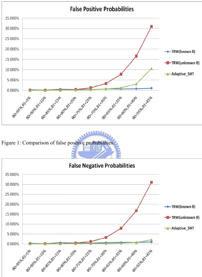
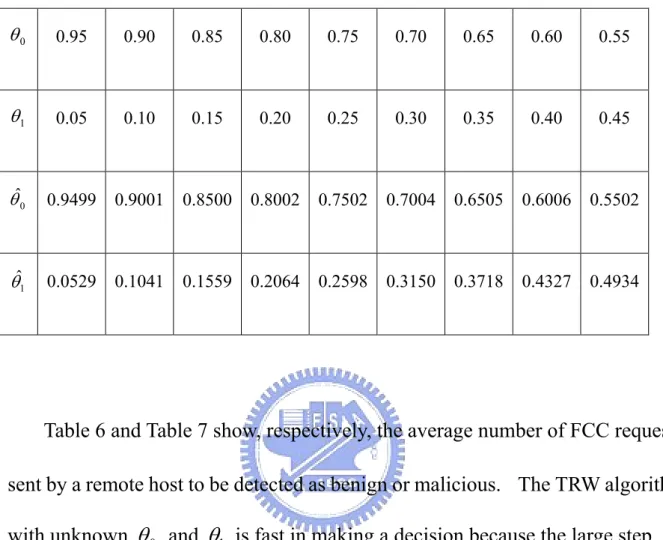
₁.

Figure 1 and Figure 2 compare, respectively, the false positive and false negative probabilities of the TRW algorithm with or without knowing

θ

₀ and

θ

₁ and our proposed adaptive algorithm, for various values of

θ

₀ and

θ

₁. We assume that

θ

₀ =0.8 and

θ

₁=0.2 are used for the TRW algorithm without knowing

θ

₀ and

θ

₁. As one can see, the false positive and false negative probabilities are very low for the TRW algorithm with perfect knowledge of

θ

₀

and

θ

₁. However, without knowing the real values of

θ

₀ and

θ

₁, its false positive and false negative probabilities of TRW could be much greater than the desired values when

θ

₀ is small and

θ

₁ is large (say,

θ

₀ =0.6 and

θ

₁=0.4). The reason is that the step size of moving upward using θˆ₀ =0.8 and θˆ₁=0.2 is significantly larger than the step size of moving upward using

θ

₀ =0.6 and

1 0.4

θ

= . Using our proposed scheme (i.e., Adaptive SHT), the false positive and false negative probabilities are almost lower than 5% for all cases (except for

0 0.55

θ

= and

θ

₁=0.45). The results are close to the desired values because the estimates of

θ

₀ and

θ

₁ in our proposed scheme are quite accurate (as Table 5 shows). Note that in our proposed scheme, the false positive probabilities are larger than false negative probabilities when

θ

₀ is large and

θ

₁ is small. This is because the number of benign hosts is much larger than the number of malicious

hosts. As a result, θˆ₀ is updated much earlier than θˆ₁. As mentioned before, the earlier detected benign hosts tend to have many more successful FCC requests

than failed ones. This implies θˆ₀ tends to be larger than the real value which

Figure 1: Comparison of false positive probabilities.

Table 5: Estimates of θ₀ and θ_{1 for the proposed adaptive algorithm.} 0 θ 0.95 0.90 0.85 0.80 0.75 0.70 0.65 0.60 0.55 1 θ 0.05 0.10 0.15 0.20 0.25 0.30 0.35 0.40 0.45 0 ˆ θ 0.9499 0.9001 0.8500 0.8002 0.7502 0.7004 0.6505 0.6006 0.5502 1 ˆ θ 0.0529 0.1041 0.1559 0.2064 0.2598 0.3150 0.3718 0.4327 0.4934

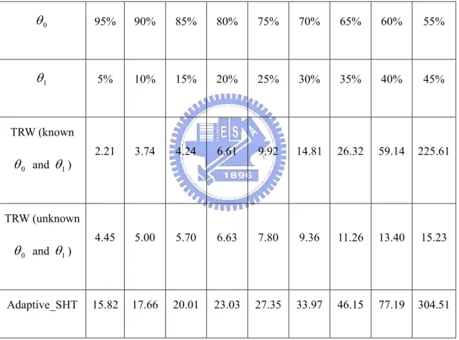
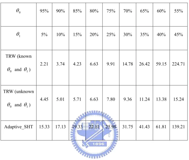
Table 6 and Table 7 show, respectively, the average number of FCC requests

sent by a remote host to be detected as benign or malicious. The TRW algorithm with unknown

θ

₀ and

θ

₁ is fast in making a decision because the large step sizes. Unfortunately, as illustrated in Figures 1 and 2, its false positive and false

negative probabilities are not satisfactory. The average number of FCC requests

for our proposed adaptive algorithm are comparable to those for the TRW algorithm with known

θ

₀ and. Let ˆθ _{and ˆ '}θ be two successive estimates of

θ

. One can stop updating ˆθ if ˆθ θ'− ˆ < for a given ε

ε

to speed up the detection time. In other words, the time spent to obtain a stable estimate of

θ

can be regarded as the period of training. Of course, to adapt to a changing

environment, the training procedure should be reactivated once in a while.

Table 6: The average number of FCC requests to detect a remote host as benign.

0 θ 95% 90% 85% 80% 75% 70% 65% 60% 55% 1 θ 5% 10% 15% 20% 25% 30% 35% 40% 45% TRW (known 0 θ and θ₁) 2.21 3.74 4.24 6.61 9.92 14.81 26.32 59.14 225.61 TRW (unknown 0 θ and θ₁) 4.45 5.00 5.70 6.63 7.80 9.36 11.26 13.40 15.23 Adaptive_SHT 15.82 17.66 20.01 23.03 27.35 33.97 46.15 77.19 304.51

Table 7: The average number of FCC requests to detect a remote host as malicious. 0 θ 95% 90% 85% 80% 75% 70% 65% 60% 55% 1 θ 5% 10% 15% 20% 25% 30% 35% 40% 45% TRW (known 0 θ and θ₁) 2.21 3.74 4.23 6.63 9.91 14.78 26.42 59.15 224.71 TRW (unknown 0 θ and θ₁) 4.45 5.01 5.71 6.63 7.80 9.36 11.24 13.38 15.24 Adaptive_SHT 15.33 17.13 19.33 22.11 25.98 31.75 41.43 61.81 139.21

Chapter 6.

Conclusion

We have presented in this paper an adaptive sequential hypothesis testing

algorithm for accurate detection of scanning worms. Numerical results show that our proposed adaptive algorithm provides accurate estimates of

θ

₀ and

θ

₁ and thus achieves false positive and false negative probabilities close to the desired values. The proposed adaptive estimation procedure for

θ

₀ and

θ

₁ is an important enhancement of the sequential hypothesis testing algorithm because it makes the algorithm much more robust to variation of

θ

₀ and

θ

₁. The

proposed adaptive detection algorithm is only suitable for scanning worms.

Bibliography

[1] J. Jung, V. Paxson, A. W. Berger, and H. Balakrishnan, “Fast Portscan Detection Using Sequential Hypothesis Testing,” In Proceedings of the IEEE Symposium on Security and

Privacy, May 9-12 2004.

[2] S. E. Schechter, J. Jung, and A. W. Berger, “Fast Detection of Scanning Worms Infections,” In Proceedings of the 7th International Symposium on Recent Advances in

Intrusion Detection (RAID 2004), September 15-17 2004.

[3] N. Weaver, S. E. Schechter, V. Paxson, “Very Fast Containment of Scanning Worms,” In

Proceedings of the 13th USENIX Security Symposium, August 9-13 2004.

[4] M. Roesch, “Snort: Lightweight Intrusion Detection for Networks,” In Proceedings of the

13th Conference on Systems Administration (LISA-99), pages 229–238, Berkeley, CA, Nov.

7–12 1999. USENIX Association.

[5] L. T. Heberlein, G. V. Dias, K. N. Levitt, B. Mukherjee, J. Wood, and D. Wolber, “A Network Security Monitor,” In Proceedings of IEEE Symposium on Research in Security

and Privacy, pages 296–304, 1990.

[6] D. Moore, C. Shannon, and J. Brown, “Code-Red: a case study on the spread and victims of an Internet worm,” in Proc. ACM/USENIX Internet Measurement Workshop, France, Nov. 2002.

http://www.caida.org/dynamic/analysis/security/nimda.

[8] D. Moore, V. Paxson, S. Savage, C. Shannon, S. Staniford, and N. Weaver, “Inside the Slammer Worm,” IEEE Magazine of Security and Privacy, 1(4): 33-39, July 2003.

[9] A. Wald, Sequential Analysis, J. Wiley & Sons, New York, 1947.

[10] R. Hogg and A. Craig, Introduction to Mathematical Statistics, The Macmillan Company, 1970.

[11] C. C. Zou, D. Towsley, W. Gong, and S. Cai. “Routing Worms: A Fast, Selective Attack Worm based on IP Address Information.” In Proceedings of the 19th Workshop on Principles of Advanced and Distributed Simulation (PADS’05), June 2005.

[12] N. Weaver, V. Paxson, S. Staniford ,and R. Cunningham. “A Taxonomy of computer worms.” In Proceedings of the 2003 ACM Workshop on Rapid Malcode, pages 11–18. ACM Press, October 27, 2003.

[13] Type I and Type II errors. From Wikipedia, the free encyclopedia, http://en.wikipedia.org/wiki/Type_I_and_type_II_errors