一設計者友善之材質設計系統

國

立

交

通

大

學

多媒體工程研究所

碩

士

論

文

一 設 計 者 友 善 之 材 質 設 計 系 統

An Artist Friendly Material Design System

研 究 生：廖仁豪

指導教授：莊榮宏 教授

林文杰 教授

一設計者友善之材質設計系統

An Artist Friendly Material Design System

研 究 生：廖仁豪 Student：Jen-Hao Liao

指導教授：莊榮宏 Advisor：Jung-Hong Chuang

林文杰 Wen-Chieh Lin

國 立 交 通 大 學

多 媒 體 工 程 研 究 所

碩 士 論 文

Submitted to Institute of MultimediaEngineering College of Computer Science

National Chiao Tung University in partial Fulfillment of the Requirements

for the Degree of Master

in

Computer Science

October 2011

Hsinchu, Taiwan, Republic of China

i

一設計者友善之材質設計系統

研究生 : 廖仁豪 指導教授 : 莊榮宏 博士

林文杰 博士

國立交通大學

資訊學院多媒體工程研究所

摘 要

An Artist Friendly Material Design System

Student: Jen-Hao Liao

Advisor: Dr. Jung-Hong Chuang

Dr. Wen-Chieh Lin

Institute of Multimedia Engineering

College of Computer Science

National Chiao Tung University

ABSTRACT

Material design is an important issue in game and animation industry. Creating an elaborate material often takes a lot of effort and time. Artists and technical artists are often involved in a material design process. Despite that there are already many successful material editors in presence, it is hard for artists to design a material on their own since current systems lack for an intuitive and sufficiently complicated material representation and an artist friendly editing system. We proposed a simple material creation flow and a material design system which are based on an intuitive material representation. Artists can bring their creativity into free play to create materials that are similar to materials in reality or even do not exist.

Acknowledgments

I would like to thank my advisors, Professor Jung-Hong Chuang and Wen-Chieh Lin, for their guidance, inspirations and encouragements. Also, I would like to thank all my colleagues in CGGM lab: Tan-Chi Ho, Tsung-Shian Huang, Jen-Chieh Liao, Bo-Yin Yao, Cheng-Guo Huang, Yi-Shan Li, Shao-Ti Lee and Mu-Shiue Li who helped me through these years. Espe-cially Cheng-Guo Huang and Tsung-Shian Huang for their advices and helped me understand the rendering knowledge. Also, I would like to thank my brother - Jen-Chieh Liao who strug-gled beside me and supported me all the way long, being as a competitor and a helpful assistant. I really appreciate all the artists and technical-artists in International Games System CO., LTD for their precious knowledge and opinions, especially Wei Lo and Yen-Tzu Chen. Lastly, I would like to thank my parents who take care of me and support me all the way long.

Contents

1 Introduction 1

1.1 Contributions . . . 3

1.2 Organization of The Thesis . . . 3

2 Related Work 4 2.1 Material Design . . . 4

2.2 BTF Compression and Rendering . . . 6

2.3 BTF Editing . . . 7

3 Approach 11 3.1 Overview . . . 11

3.2 Material Representation . . . 13

3.3 Material Creation Flow . . . 16

3.3.1 Geometry Part . . . 16 3.3.2 Diffuse Part . . . 18 3.3.3 Specular Part . . . 19 3.4 User Interface . . . 28 3.4.1 Object Preview . . . 29 3.4.2 Specular Design . . . 31

3.4.3 Parameter Control Part . . . 32

4 Results 34

4.1 Rendering . . . 34

4.2 Comparison and Editing Effects . . . 36

4.2.1 BTF Comparison . . . 36 4.2.2 Material Editing . . . 40 4.3 Editing Samples . . . 53 5 Conclusion 68 5.1 Summary . . . 68 5.2 Limitations . . . 69 5.3 Future Works . . . 69 Bibliography 71 iv

List of Figures

2.1 The material editor in Unreal Engine . . . 5

2.2 Material modeling pipeline . . . 6

2.3 Edit propagation pipeline . . . 8

2.4 SPMM edit pipeline . . . 9

3.1 Material creation flow of our work . . . 12

3.2 BTF decomposition workflow . . . 13

3.3 The specular color is stored in a parabolic map and accessed by the half vector . 15 3.4 The material representation . . . 15

3.5 The creations of normal map and height map . . . 16

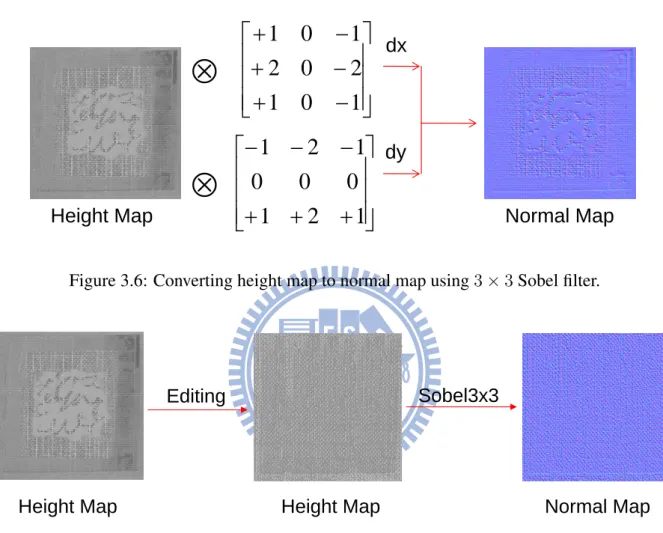
3.6 Converting height map to normal map using 3 × 3 Sobel filter . . . 18

3.7 Using “clone tool” to edit the height map . . . 18

3.8 The process for generating the diffuse color map . . . 19

3.9 Design interface for specular maps . . . 20

3.10 The indications of theta and phi angle . . . 21

3.11 The process to get the specular mask map and Fresnel map . . . 21

3.12 The graph of the Fresnel term to the angle degree between L and H (with r0 = 0.5) 22 3.13 Two cases that make a material appear brighter . . . 23

3.14 The shape of (L · N + V · N − (L · N )(·N )) . . . 23

3.15 The meaning of tilted reflection map . . . 24 v

3.16 Using “Adjust Color Curves” tool to change the reflection at grazing angle . . . 25

3.17 The anisotropic reflection of a watch . . . 26

3.18 The meaning of the rotation map . . . 26

3.19 Filtering process of different rotation map representations . . . 27

3.20 The color selection interface of GIMP . . . 28

3.21 Drawing a 360 rotation via “Draw 360” button. . . 28

3.22 User interface . . . 29

3.23 The menu bar icons . . . 29

3.24 The control panel of the lighting and viewing directions . . . 30

3.25 Changing the type of light source . . . 30

3.26 “Expand window” button demonstration . . . 31

3.27 Specular design window indication . . . 32

4.1 The comparison of different rendering methods for wallpaper . . . 37

4.2 The comparison of different rendering methods for WL cool . . . 39

4.3 The material creation flow of WL cool . . . 40

4.4 Changing the height map of wood . . . 41

4.5 Using “Blur/Sharpen” brush tool to smooth the higher region of the material . . 41

4.6 Using “Interactive Warp” to warp the height map counterclockwisely . . . 42

4.7 Changing the color of the material . . . 43

4.8 Comparison between the effect of specular mask map and Fresnel map . . . 44

4.9 Changing tilted reflection map . . . 45

4.10 Enhancement of the tilted reflection appears in a certain range . . . 46

4.11 Specially designed specular color maps . . . 47

4.12 Using specular color maps to produce rim light effects . . . 48

4.13 Using another specular color map to produce the lacquer appearance . . . 49

4.14 Using rotation map to create brushed metal effect . . . 50

4.15 Using rotation map to make special effect . . . 51

4.16 Using rotation map to reduce the number of specular color maps . . . 52

4.17 Minor translucent material . . . 55

4.18 Disk . . . 56 4.19 Corduroy . . . 57 4.20 Wallpaper . . . 58 4.21 Wool . . . 59 4.22 Glossy hemp . . . 60 4.23 Hemp . . . 61

4.24 Beige glossy leather . . . 62

4.25 Rusty iron . . . 63

4.26 Lava liked material . . . 64

4.27 Artificial porcelain vase . . . 65

4.28 Wood . . . 66

4.29 Wood with lather . . . 67

C H A P T E R

1

Introduction

Materials such as brick, wood or cloth are everywhere in game and animation. It is an important feature to enrich our digital world and makes objects look alive. Thus, creating an appealing rendering result of a material is crucial. Note that an appealing rendering result is not necessarily photo-realistic, since the world in game and animation is often full of imagination.

Material design is not an easy task. It often involves two main roles: artist and technical artist. Artist designs the base textures and the technical artist designs the lighting phenomena of the material using the base textures as the input. Some parameters are then tuned by the artists for the fine rendering result. Although several successful material editors have been developed, it is still hard for the artists to really manage the tools since the control of the appearance of a material is restricted to the parameters which are provided by the technical artist. Since there are no intuitive material representations and artist friendly editing tools to design the appearance of a material, several passes back and forth between artist and technical artist should be done to design an appealing material.

When considering the rendering of a material in reality, bidirectional texture function (BTF) proposed by Dana et al. [DVGNK99] would be a good choice. BTF is a six-dimensional

2 function, involving lighting, viewing direction, and position. Due to the fact that all the data are captured from a real material, BTF can produce photo-realistic appearance. Many methods have been proposed to compress the BTF data. Some of the methods also come with some editing capabilities which are, however, usually limited. Such editing tools usually lack the editing abilities of a drawing system which is much more friendly for an artist.

Menzel and Guthe [MG09] proposed a novel representation, called geometric BRDF (g-BRDF), that decomposes the BTF data into meso- and micro-scale properties represented by textures. User can use any image manipulation tool to edit the texture to affect the appearance of the material. Although g-BRDF allows user to design a material by updating the associated textures, which are in our experience quite time consuming. Also, some of the parameters of the g-BRDF are not quite intuitive for artists to manipulate. On the other hand, BTF data can not be obtained easily for general people. For some cases, for example, materials that do not exist in reality, it is even impossible to acquire. These observations motivate us to study the feasibility of designing general materials via a single or a few images and involving less effort of the technical artists.

In this thesis, we proposed a simple material creation flow and a material design system based on an intuitive material representation. The representation consists of the geometry part, diffuse part and specular part of the material. Such intuitive representation allows artists to design a material without much difficulty. Given a single or a few images, an artist can first generate the textures that represent the materials by using some image processing tools. Then manipulate and refine each texture using the proposed design system. The design system is implemented as a plugin of an image manipulation program, thus all the manipulations can be viewed in real-time and the editing tools are much friendly to the artist. The capabilities of the editing tools are not restricted to what are currently provided; any other plugins can be merged to strengthen the design process. With the proposed system, artists can bring their creativity into free play to design complex materials intuitively with flexible controls over the surface appearance.

1.1 Contributions 3

1.1

Contributions

We proposed an artist friendly material design system that allows artists to design complex materials based on a single or a few images. By extending g-BRDF material representation, the system provides a framwork on which artists can design mimic appearance of a complex material without the BTF data or even materials that are not existent in reality. More flexible controls over the specular effect of the material are also provided. For example, Users can control the reflection phenomena at a grazing angle, or produce minor translucent effect or perturbation effect on the material. Complex speucular phenomena which rotate around the surface (e.g., watch and disk) can also be produced easily.

1.2

Organization of The Thesis

The following chapters are organized as follows: Chapter 2 gives a literature review and related background knowledge. Chapter 3 introduces our framework and the details of the system. Chapter 4 shows the results of our method. Finally, we summarize our work and discuss future works in Chapter 5.

C H A P T E R

2

Related Work

2.1

Material Design

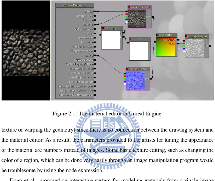
In recent years, computer graphics have been vigorously developed. It has been seen widely in games, movies and animations. The research on material designing is of great worth. Cur-rently, in game and animation industry, some successful software and application programming interfaces (e.g., Unreal Engine, Frostbite Engine and RenderMan) provide a node based shader synthesis tool to edit the appearance of a material (Figure 2.1). User can design the appearance of a material via linking some operators (e.g., multiply, add...) and operands (e.g., texture, tex-ture coordinates, constant...) in a way visual programming does. Such connectivity is called a node expression. A shader code will be automatically generated from the node expression for rendering the material, thus user can design and render a material without knowing how to write a shader code. User can create a node expression which is well tailored to a specific material. However, knowing how to manipulate all the operators and operands to create a material needs a lot of experiences and the knowledge of computer graphics. It is difficult for an artist to design such expression. Also, the manipulation of the operands itself is not provided (e.g., painting the

2.1 Material Design 5

Figure 2.1: The material editor in Unreal Engine.

texture or warping the geometry) since there is no connection between the drawing system and the material editor. As a result, the parameters provided to the artists for tuning the appearance of the material are numbers instead of images. Some basic texture editing, such as changing the color of a region, which can be done very easily through an image manipulation program would be troublesome by using the node expression.

Dong et al. proposed an interactive system for modeling materials from a single image (Figure 2.2) [DTPG11]. Given a single image lit by a directional light source with known direction, the method first interactively separates the image into an albedo map and a shading map, then reconstructs the normal from the shading map to recover the geometric features. Specular parameters are finally assigned to each pixel guided by user strokes and the diffuse albedo to reproduce the appearance of a material. Although user can reproduce the appearance of a variety of materials, such scheme can not handle complex specular phenomena which rotate around the surface (e.g., watch). Also, the system does not provide more sophisticated editing abilities which are crucial for material design.

2.2 BTF Compression and Rendering 6

Figure 2.2: Material modeling pipeline. Adopted from [DTPG11].

2.2

BTF Compression and Rendering

To represent a material in reality, Dana et al. [DVGNK99] introduced the BTFs. It is obtained by taking lots of photos under different lighting and viewing directions. The storage for a single material may cost several gigabytes. Such enormous data size is not suitable for current graphics hardware for rendering a BTF. Thus several methods have been proposed to compress the BTF data.

The compression methods can be roughly divided into three categories: linear factoriza-tion based [MMK03b, SBLD03, KMBK03, MCT+05, VT04, WWS+05], probabilistic model based [HF03, HF04, HFA04, HF07, HH10] and pixel-wised BRDF based [McA02, MMK03a, MMK04, MCC+04, FH04, FH05, CCCC08, MG09, WDR11]. Linear based methods use prin-cipal component analysis (PCA), singular value decomposition (SVD) or other matrix factor-ization methods to approximate the original data. They reduce the high-dimensional input data to low-dimensional subspaces containing most of the information. The resulting eigenvectors can be stored into texture maps. Thus BTF can be rendered in real time while preserving good visual quality. Probabilistic model based methods provide large compression ratio and allow for seamless spatial enlargement. However, linear factorization based and probabilistic model based methods do not offer meaningful parameters to control the appearance of the material. On the other hand, pixel-wised BRDF based methods try to fit the BTF data to physically

meaning-2.3 BTF Editing 7 ful BRDF model which are useful for editing purpose. McAllister [McA02] approximated the BTF data by fitting a Lafortune BRDF model [LFTG97] for each texel. However, this method assumed the surface is nearly flat that excludes the self-occlusion, self-shadowing and inter-reflection effects. Without the knowledge of the meso-geometry of the material, these kinds of effects would all be considered as general reflection results. Thus BTF is much equivalent to spatially varying BRDF (SVBRDF). For bump surfaces, this method would not be suitable as the effects caused by the meso-geometry can not be correctly modeled by any BRDF model which assumes reciprocity and energy conservation. Nonetheless, Lafortune model has been modified and extended in other pixel-wised BRDF compression methods to approximate the BTF for those materials that have greater depth variation. Meseth et al. used a non-linear function similar to the Lafortune model [MMK03a, MMK04], Filip and Haindl developed a polynomial extension of one lobe Lafortune model to approximate the reflectance fields of BTF [FH04, FH05]. Besides the Lafortune model, Ma et al. used Phong model to get an average surface BRDF [MCC+_{04]. The difference between the original data and the fitting results of the}

Phong model (a spatial-varying residual function) is approximated by a specific delta function. Based on the observation that self-shadowing is view independent and self-occlusion is lighting direction independent, Chen et al. approximates the BTF by an SVBRDF incorporating shad-owing and occlusion information [CCCC08]. For detailed survey on BTF compression, please refer to [FH09] and [MMS+05].

2.3

BTF Editing

BTF acquisition is not an easy task, thus BTF editing would have its own practical demands. Currently, BTF editing can be roughly divided into two approaches: Direct editing approach [KBD07, XWT+09] and fitting approach [MG09, WDR11]. In [KBD07] an out-of-core data management for editing raw BTF data is proposed. They provided sophisticated operators to edit the BTF appearance such as shadows, specularity and meso-structure. However, the main drawback of this approach is that if the meso-geometry of the material is changed, the

corre-2.3 BTF Editing 8 sponding feature (e.g., shadows) does not change accordingly. Xu et al. proposed a BTF editing method using an edit propagation scheme [XWT+_{09], in which the user first edits a small region}

on a certain slice of BTF and then the editing will be propagated to the positions that have sim-ilar feature. View independent features such as normals and reflectance features reconstructed from each view are used to guide the propagation process; see Figure 2.3. Since the method does not rely on explicit geometry, it allows user to edit BTF with non-height field geometry. However, without the geometry information, the control over the meso-geometry of the BTF is not allowed. Although direct editing approaches provide interactive editing of raw BTF data, they can not directly edit the compressed data.

Figure 2.3: Edit propagation pipeline. Adopted from [XWT+09].

2.3 BTF Editing 9 advantageous since BRDF models provide physically meaningful parameters for user to con-trol. However, previous works either fit the BTF data using a single BRDF model or do not consider the underlying meso-geometry of the surface. Therefore, they usually lose a great of accuracy. Recently, Wu et al. [WDR11] proposed a Sparse Parametric Mixture Model (SPMM) to represent general BTFs. They adopted the stagewise Lasso algorithm to fit multiple, rotated analytical BRDFs of different types to the BTF data (Figure 2.4). This representation preserves

Figure 2.4: SPMM edit pipeline. Adopted from [WDR11].

the BTF appearance while the storage size remains compact. The editing task is accomplished via changing the parameters of all the analytical models. However, without the height field to store the meso-geometry information, the control over the meso-geometry of the material is not provided.

2.3 BTF Editing 10 Most current BTF editing approaches need a specific user interface tailored for a specific algorithm to accomplish the editing task. Although such a user interface can provide simple editing such as color change, specular intensity or rougher the surface, edits are often affected globally. There are no artist friendly tools to edit a certain region. Also, since the user interface does not a drawing system, editing would not be intuitive and friendly for artists. On the other hand, Menzel et al. [MG09] proposed a novel way called g-BRDF to represent a BTF. The BTF data is decomposed into a height map which describes the surfaces’ meso-geometry and some other maps that store the BRDF parameters. By carefully estimating the BRDF parameters and height field, this method provides high compression rate and good rendering quality. Since all the parameters are stored in texture maps, this approach provides a more flexible editing capability than other approaches. The editing process is not restricted to specific editing tools; user can choose any image manipulation program to edit the textures of the g-BRDF. However, without combining to an appropriate drawing system, editing a material would require a lot of efforts. Every time when a texture is edited, manually reload the texture would be required to see the changes. Also, the meaning of the normal distribution function is not clear for the artists to deal with. It would be hard for an artist to create a material directly from the scheme of the g-BRDF. This motivates us to develop a design system that allows artists to create general materials (real or unreal) intuitively and easily.

C H A P T E R

3

Approach

In this chapter, we first give an overview, then introduce the material representation, and finally the proposed artist friendly material design system.

3.1

Overview

To let an artist intuitively create a material and edit its lighting phenomena, it is necessary to have the following features:

1. Artist friendly material representation. 2. Artist friendly editing tools.

3. Real-time feedback.

4. An easy to use intuitive user interface.

Considering all the above features, we implement our system as a GIMP (GNU Image Manip-ulation Program) plugin. GIMP is a free raster graphics editor. It is primarily employed as

3.1 Overview 12 an image retouching and editing tool. In addition to detailed image retouching and free-form drawing, GIMP can accomplish some essential editing tasks such as resizing, editing, cropping photos, and conversion between different formats. Thus we can utilize GIMP to manipulate the images without writing our own drawing system.

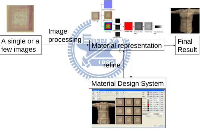
The proposed material creation flow can be depicted in Figure 3.1. Given a single or a few images, we first generate the textures that represent the material’s meso-geometry, diffuse part, and specular part. Then we manipulate and refine each part using the proposed system to design the desired material.

A single or a

few images

Material representation

Material Design System

refine

Image

processing

_Final

Result

3.2 Material Representation 13

3.2

Material Representation

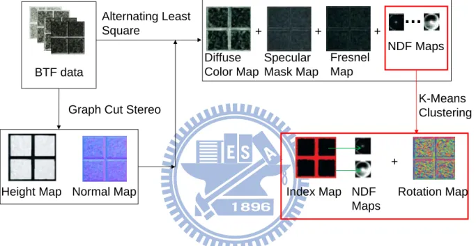
We use the g-BRDF proposed by Menzel and Guthe [MG09] with slightly modification to represent a material due to its photo-realistic BTF rendering result and intuitive data represen-tations. The decomposition of a BTF is shown in Figure 3.2. For a given BTF data, they first

Alternating Least Square + NDF Maps + K-Means Clustering NDF Maps BTF data

Height Map Normal Map Graph Cut Stereo

Index Map Rotation Map + Diffuse Color Map Specular Mask Map Fresnel Map +

…

Figure 3.2: BTF decomposition workflow.

extract the meso-geometry (height map and normal map) of the material by using graph cut stereo [RC98] and then fit the BTF data to a BRDF model with the meso-geometry information considered. The BRDF model that g-BRDF employed is the Ashikhmin’s distribution-based BRDF [Ash06]. It provides a good approximation of many real world materials with quite intuitive meaning. The BRDF is defined as follows:

ρ(L, V ) = Cd π +

Cs maskp(H)F (L · H)

L · N + V · N − (L · N )(V · N ), (3.1) where L is the lighting direction, V is the viewing direction, H is the half vector, Cdis the

3.2 Material Representation 14 F (L · H) is the Schlick’s Fresnel term:

F (L · H) ≈ r0 + (1 − r0) × (1 − L · H), (3.2)

where r0is the reflectance at normal incidence. All the parameters are stored into texture maps:

Cd is stored into a diffuse color map, Cs mask is stored into a specular mask map, p(H) is

stored into a NDF map and r0 is stored into a Fresnel map. After the fitting, we can get the

diffuse color map, specular mask map, Fresnel map and lots of NDF maps. Each NDF map corresponds to each pixel of the image (for a 2562 × 812 _{BTF, the number of the NDF maps}

would be 256 × 256). To reduce such enormous data size, k-means clustering is applied. It reduces all the NDF maps to be approximated by some NDF maps with different rotations around the center. The index map indicates which NDF Maps is used for that pixel and the rotation map stores the rotation that needs to be applied. Thus, to reproduce the NDF map of a pixel, we first get the corresponding NDF map by using the index map, then rotate the NDF map around the center with the degree stores in the rotation map.

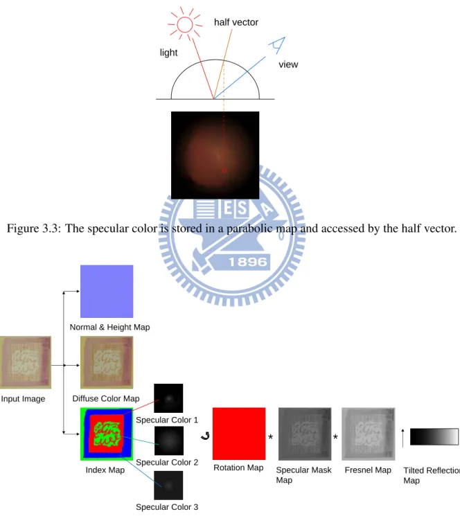
The normal distribution function of the Ashikhmin’s distribution-based BRDF describes how much percentage of the micro-facet normal equals to the given half vector. It is stored in a parabolic map and accessed by the half vector. Thus the higher the value is, the more the energy reflected directly toward the viewing direction. To obey the energy conservation, the sum of all probabilities (the integral over hemisphere) cannot exceed one. However, this information is quite obscure for artists to manipulate. We have found that the normal distribution function in g-BRDF contained color information for better fitting results. Thus if we relax the constraint (the integral over hemisphere can exceed one) and multiply the distribution by a smaller Cs mask

to approximate the condition (the integral over hemisphere cannot exceed one), the normal distribution function can be interpreted as the specular color which depends only on the half vector ((L + V )/2). Thus p(H) is replaced by Cs(H) in our representation, where Csindicates

specular color. We store the specular color in the parabolic map (Figure 3.3), leading to a more uniform texel sampling on the upper hemisphere compared to the sphere map, and even to the cubical map. In addition to that, we also introduce another map called “Tilted Reflection Map”

3.2 Material Representation 15 to control the reflection of the material at grazing angle. We will give more details about the tilted reflection map in the following section. Finally, our material representation can be shown in Figure 3.4.

light

view half vector

Figure 3.3: The specular color is stored in a parabolic map and accessed by the half vector.

* *

Input Image

Normal & Height Map

Diffuse Color Map

Index Map Specular Color 1 Specular Color 2 Specular Mask Map Fresnel Map Specular Color 3

Rotation Map _{Tilted Reflection} Map

3.3 Material Creation Flow 16

3.3

Material Creation Flow

In this section, we describe how we obtain all the texture maps we need for our representation and how we use the textures and design system to enhance the design of a material. The material creation flow can be separated into three main parts: Geometry Part, Diffuse Part and Specular Part.

3.3.1

Geometry Part

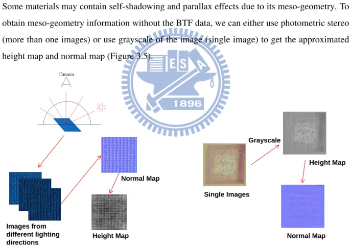
Some materials may contain self-shadowing and parallax effects due to its meso-geometry. To obtain meso-geometry information without the BTF data, we can either use photometric stereo (more than one images) or use grayscale of the image (single image) to get the approximated height map and normal map (Figure 3.5).

Images from different lighting directions Normal Map Height Map Single Images Height Map Normal Map Grayscale

Figure 3.5: The creations of normal map and height map. Left: Photometric Stereo. Right: grayscale approximation.

3.3 Material Creation Flow 17 For the photometric stereo, the method assumes the material as a Lambertian surface and illuminated from a distant small source. The normal can be solved by inverting the linear equation:

I = N · L, (3.3) where I is a vector of the intensities for a pixel in m images, N is the surface normal, and L is a 3 by m matrix of normalized lighting directions. The normal integration method proposed by Frankot and Chellappa is then applied to recover the height map [FC88].

For materials with less specular and similar colors, using grayscale of the image can produce approximated meso-geometry quite well. To use the grayscale of an image as the height map, it is important that the material is lit evenly from any direction to avoid the shadowing effect and specular effect. Thus the intensity of a texture would be highly corresponding to the ambient occlusion rate (the darker the deeper) and hence can be used to approximate the height map. GIMP already has a plugin that can be utilized to generate the normal map from a height map. However, the approximated geometry may not be accurate. Artists may also wish to make the material smoother or rougher. For these purposes, the ability to edit the geometry is necessary. To keep the consistency between the normal and height field, users have to manually rebuild the normal map via GIMP plugin every time when the height map is changed. To solve this problem, we actually store the height map only and calculate the normal map using 3 × 3 Sobel filters at runtime (Figure 3.6). By convoluting the height map with the Sobel filters, we can get the derivative of the x direction (dx) and the derivative of the y direction (dy). The derivative of the z direction (dz) can be calculate via 1 −p(dx2_{+ dy}2_{). Thus the normal at a pixel would be}

(dx, dy, dz). However, artists may wish to strengthen the geometry feature, so we actually get our normal by normalizing the vector (dx, dy, 1.0/N ormalStrength) with N ormalStrength ranges between 1.0 to 8.0. Since we calculate the normal map at runtime, user can see the changes on the fly without manually rebuilding the normal map.

For the wallpaper sample, the height map using grayscale of the image is not quite accurate. From the observation of the wallpaper BTF data, we know that the meso-geometries are all the same over the surface. The white area and the golden part in the middle should have the same

3.3 Material Creation Flow 18 meso-geometry as the periphery. Thus we use “clone tool” of GIMP to clone the height field of the periphery to the middle part as shown in Figure 3.7.

Height Map

Normal Map



































1

0

1

2

0

2

1

0

1

































1

2

1

0

0

0

1

2

1



dx

dy

Figure 3.6: Converting height map to normal map using 3 × 3 Sobel filter.

Editing

Sobel3x3

Height Map

Height Map

Normal Map

Figure 3.7: Using “clone tool” to edit the height map. The contrast of the height map is en-hanced for better observation.

3.3.2

Diffuse Part

For the diffuse part, we assume the surface is perfectly diffuse that scatters incident light uni-formly in all directions. Thus we use the same image which we take for the geometry part as our diffuse color map. Usually we will decrease the intensity of the diffuse color map to exclude the specular intensity. Editing may be applied to further modify the results (Figure 3.8).

3.3 Material Creation Flow 19

Decrease

Intensity Editing

Original Image Initial Diffuse Color Map Final Diffuse Color Map

Figure 3.8: The process for generating the diffuse color map.

3.3.3

Specular Part

Index Map The specular part of our representation consists of an index map, a specular mask map, a Fresnel map, a tilted reflection map and a few specular color maps. From the observa-tions of the index maps for different materials in [MG09], we found that the regions which have similar diffuse colors share the same index. Thus we can use color selection tool, edge detec-tion, color mapping/remapping tools or any other image processing tools of GIMP to separate the image into similar parts easily. The segmented parts are then indexed by an index map. Each channel of the index map represents the weight for each specular color map (Equation 3.4). For example, in the index map of the wallpaper, as shown in Figure 3.4, the pure red region corresponds to specular color 1 and pure green region corresponds to specular color 2,..., and so on.

Cs= IndexM ap.r × Cs 1+ IndexM ap.g × Cs 2+ IndexM ap.b × Cs 3 (3.4)

Specular Maps After the segmentation, the next step would be the design of the specuar color map for each region. As stated in Section 3.2, we store the specular color in a parabolic map that is accessed by using the half vector. Although using half vector for deciding the specular color is much easier, it would still be too difficult for artists to design the parabolic map. It is not clear for artists to be aware which texel of the parabolic map is accessed for a given lighting and viewing directions. To tackle this problem, our system provides a special design window which has nine viewports showing the results of different lighting and viewing direction over the upper

3.3 Material Creation Flow 20 hemisphere (Figure 3.9). Each viewport corresponds to a different phi angle (Figure 3.10) of the lighting and viewing directions, allowing artists to change the theta of lighting and viewing directions. To let the artist acknowledge which pixel of the specular color map corresponds to the current lighting and viewing directions, we mark it as red points at the “Specular Position” block at the bottom right. Artist can draw the parabolic map and get the feedback right away in real-time with the corresponding pixels of the specular color map under different lighting and viewing direction indicated.

3.3 Material Creation Flow 21

x

y

z

ψ

θ

Figure 3.10: The indications of theta and phi angle.

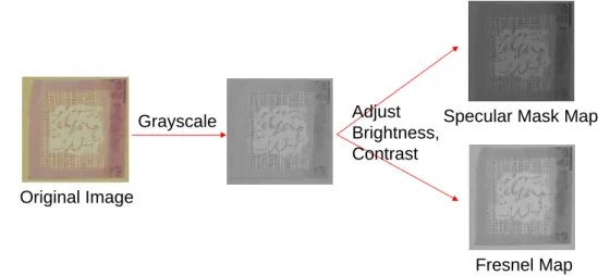
Specular Mask Map The obtained specular color map would be multiplied with the specular mask map to control its intensity. Generally, for a material that is lit evenly from any direction, a position that has a higher intensity value tends to have a lower ambient occlusion rate or a higher reflection rate. Thus we use the intensity of the diffuse color map as the initial specular mask map and change the brightness and contrast via our design system for better results (Figure 3.11).

Grayscale Specular Mask Map

Fresnel Map Adjust

Brightness, Contrast Original Image

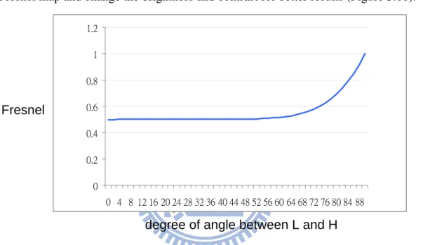
3.3 Material Creation Flow 22 Fresnel Map The Fresnel term expresses the reflection of light on material, which Schlick’s Frensel is used. The Fresnel term increases from r0to 1 as the angle between L and H increases

from 0 to 90 degree (Figure 3.12). Hence the material will become brighter when it is illumi-nated at the grazing angle and viewed from the opposite side (Figure 3.13 left). Similar to the creation of the specular mask map, we also use the intensity of the diffuse color map as the initial Fresnel map and change the brightness and contrast for better results (Figure 3.11).

Fresnel

degree of angle between L and H 0 0.2 0.4 0.6 0.8 1 1.2 0 4 8 12 16 20 24 28 32 36 40 44 48 52 56 60 64 68 72 76 80 84 88

Figure 3.12: The graph of the Fresnel term to the angle degree between L and H (with r0 = 0.5).

Tilted Reflection Map Besides the tilted reflection case as shown in Figure 3.13 left, the material should also appear brighter when it is illuminated at the grazing angle and viewed from the same side (Figure 3.13 right). However, this effect is not described in the Fresnel term. No matter how tilted the lighting and viewing directions are, as long as they are the same, the Fresnel term would be all the same since it only depends on the degree between L and H. To enhance these kinds of lighting effects, Ashikhmin’s distribution-based BRDF [Ash06] divides the specular part by (L · N + V · N − (L · N )(V · N )). The shape of the divisor is shown in Figure 3.14. The divisor ranges between 0 and 1, thus the specular will be amplified when either the angle between lighting direction and the normal or the angle between viewing direction and the normal becomes larger. Considering the design purpose for unreal materials for gaming and

3.3 Material Creation Flow 23

L

V

L

V

Figure 3.13: Two cases that make a material appear brighter. Usually the case at the left is brighter than the case at the right.

L dot N

V dot N

3.3 Material Creation Flow 24 animation industry, artists may wish to further control this amplified phenomenon. Thus we store the value of cos(θ), given θ from 0 to 90, as a 91 × 1 texture. Given L · N or V · N , we first calculate the angle using arccos then use it as the texture coordinate to access the value of the dot product which stores in the texture (Figure 3.15). Linear filter is applied to the texture to linearly interpolate the value between each texel. For more intuition (the whiter the brighter), we store 1 − cos(θ) in the texture instead of cos(θ). Artists can use the default button to set the value of 1 − cos(θ) to the texture and use the “Adjust Color Curves” tool to easily edit the slope (Figure 3.16).

‧‧‧

θ = 0 1 2 3 4 5

‧‧‧

85

86

87

88

89

90

N

L or V

θ

1-cos(θ) =

Figure 3.15: The meaning of tilted reflection map. We store the value of the dot product in the texture, allowing user to control the phenomenon of tilted reflection (we store 1 − cos(θ) instead of cos(θ)).

3.3 Material Creation Flow 25

Tilted Reflection Map Tilted Reflection Map

Figure 3.16: Using “Adjust Color Curves” tool to change the reflection at grazing angle. Left: default settings. Right: specify the tilted reflection starting at the lower angle).

Rotation Map Up to now, we can handle general anisotropic materials and isotropic materi-als. But when dealing with some special materials whose specular changes continuously over the phi angle (e.g., watch (Figure 3.17)), it would be hard to use some discrete specular colors for approximation. To solve this problem, rotation map is introduced. Each texel of the Rotation map stores the rotation of the corresponding specular color map (Figure 3.18). The rotation is encoded as hue in HSV color space. Some may consider why not use a gray scale image which maps 0-255 to 0-359 degree to encode the rotation angle. The reason is that, when considering the mipmap filtering, the rotation degree would be wrong in some cases. For example, given 4 pixels in which all the top pixels are 0 degree and all the bottom pixels are 359 degree (Figure 3.19). The filtered color between 0 degree and 359 degree would be 180 degree which is far

3.3 Material Creation Flow 26

Figure 3.17: The anisotropic reflection of a watch.

Index Map Specular Color Map Rotation Map

45°

HSV color space Rotated Specular Color Map

3.3 Material Creation Flow 27 0 degree 359 degree 0 degree 359 degree RGB(0,0,0) RGB(255,255,255) RGB(255,0,0) RGB(255,0,4) Filter Filter 180 degree 0 degree RGB(128,128,128) RGB(255,0,2) Gray scale HSV color space

Figure 3.19: Filtering process of different rotation map representations.

from either 0 or 359 degree. However, if we store the degree as hue in HSV color space, the color of 0 degree and the color of 359 degree are almost identical, thus we have the correct degree after filtering. On the other hand, the color selection interface of GIMP provides the information of HSV and the corresponding RGB color at the same time (Figure 3.20). This really breaks the gap for user to understand which color corresponding to which degree and vice versa. However, drawing a rotation map that rotates around the center is really difficult. To solve this problem, we provide a button which can draw a 360 rotation around the center of a region specified by the users (Figure 3.21).

3.4 User Interface 28

degree

RGB

Figure 3.20: The color selection interface of GIMP.

Figure 3.21: Drawing a 360 rotation via “Draw 360” button. When the button is pressed, a 360 rotation around the center of the selected region will be drawn automatically.

3.4

User Interface

Our user interface is shown in Figure 3.22. From left to right, we can roughly divide the inter-face into three parts: object preview, specular design and parameter control.

3.4 User Interface 29

Figure 3.22: User interface.

3.4.1

Object Preview

In order to allow artists to clearly observe the outcome of their design, we provide an object preview window on which several basic models; Quad, Cube, Sphere, Torus and Teapot can be selected. User can select the model from the menu bar or load the desired model using “Load model” button (Figure 3.23). Changing lighting and viewing directions are allowed via

Wheel type switch

Reset button Expand window

Object selection

Load model

Point light toggle

Figure 3.23: The menu bar icons.

3.4 User Interface 30 (Figure 3.24).

Figure 3.24: The control panel of the lighting and viewing directions.

The “Wheel type switch” at the menu bar is used to switch the control between viewing radius and lighting radius when controlled by the mouse wheel. User can use the “Reset but-ton” to reset the viewing and lighting directions to the default values. To cover any viewing and lighting degrees, theta can be set in the range of −180 and 180 degree and phi can be set in the range of 0 and 360 degree. When “auto” check box of a specific parameter is checked, the corresponding degree will automatically increase to the maximum and back to the minimum. Artists can see the dynamic change of the lighting and viewing direction while editing at the same time. Note that the control of the parameters is synchronized; user can observe the cor-responding degree no matter which control method is used. By default, the type of the light source is set to directional light. However, user can change the light source to point light source via the “Point light toggle” button (Figure 3.25).

Directional Light Point Light

3.4 User Interface 31 The “Expand window” button at the menu bar is designed for users who use small monitors or less efficient graphic cards. When it is clicked, the specular design window will be hidden and the object preview window expanded. User can then resize it to a smaller window (Figure 3.26). Clicked it again will bring back the specualr design window (Figure 3.22).

Figure 3.26: “Expand window” button demonstration.

3.4.2

Specular Design

The part for specular design is mainly used for specular color design. The nine viewports correspond to different lighting and viewing directions over the upper hemisphere (Figure 3.27). Phi angle is fixed while theta can be set in the range of 0 and 90 degree. When “auto” of a specific parameter is checked, different from the object preview window, the degree will increase to the maximum then decrease to the minimum to avoid the unlighted angle.

3.4 User Interface 32

Phi = 0

Phi = 45

Phi = 90

Phi = 135

Phi = 180

Phi = 225

Phi = 270

Phi = 315

theta = 0

Figure 3.27: Specular design window indication.

3.4.3

Parameter Control Part

The upper right block of the user interface is the map selection block. This block is used for map selection and continuous texture updating. When “Update” of a specific texture is checked, any editing to the texture will directly affect the result. All the maps selected will be memorized. Thus if we accidently close the plugin, there is no need to reselect textures again when we re-execute the plugin. To speed up the map selection process, we filtered the map by its filename such that only those maps containing the key words (e.g., Height) in their filenames are displayed for selection. We only display all the opened maps for selection if none of the maps match the key word.

The “Parallax Occlusion Mapping” block provides the parameters required for parallax oc-clusion mapping, such as height map scale and texture repeat times. Height map scale is the ratio of height to width, which is used to map the height from the range {0.0, 1.0} to a range better represents the physical properties of the surface being simulated. For instance, a brick wall texture might cover a 2 × 2 meter area and the surface of the bricks give the surface a

3.4 User Interface 33 thickness of 0.02 meter. The height map scale for this material would be 0.02/2 = 0.01.

“Tilted Reflection” block provides a button that can be used to set the tilted reflection map to the default values. Artist can design the tilted reflection map via editing the default values (Figure 3.15 and 3.16).

“Rotation Map” block provides a button that can help user to create a 360 rotation around the center of the selected region (Figure 3.21).

“Normal Map Strength” block provides a spin button which is used to set the N ormalStrength for normal map calculation (Subsection 3.3.1). The higher the value is, the stronger the geom-etry features are.

“Specular Position” block will appear when any of the specular color maps is set to be updated continually. This block indicates the specular color positions corresponding to the viewports of the specular design window (Figure 3.9)

C H A P T E R

4

Results

In this chapter, we first describe some details about rendering, then we compare our results to the BTF and show the effects of editing operations. Finally, we show some of the results which are created via our material design system.

4.1

Rendering

We implement the proposed design system by using OpenGL with glsl shading language and put it on top of the GIMP as a plugin. Considering the real-time feedback, which is crucial for an artist friendly design system, we carefully manage the resources. As a result, we share the same texture objects and shader context for the object preview window and specular design window. Also, to reduce texture accesses times, all the specular color maps are combined into a 2D texture array. When changes are applied to a specific specular map, we only update the corresponding layer of the 2D texture array rather than regenerate the whole texture array.

For realism, we apply Parallax occlusion mapping [Tat06] to simulate the self-shadowing effect of the material. This algorithm needs tangent and binormal vectors to transform the light

4.1 Rendering 35 and view vectors to the tangent space for ray tracing. Since our focus is on the appearance of static objects, there is no need to calculate them every time for each frame. When a model is loaded, we first calculate the tangent for each vertex and then obtain the binormal via the cross product of the normal and tangent. However, direct calculation of the tangent for each face may not generate appealing results since the tangents for those faces that share the same vertex are not equal. As a result, the seams between surfaces are quite obvious, especially for round objects (e.g., ball). To solve this problem, the smoothness over the tangent is needed. Note that if we directly sum up all the tangents sharing the same vertex, it would also produce incorrect result for objects that have sharp edges (e.g., cube). Thus we only sum the tangents that share the same attributes (normal, texture coordinate and vertex position) for smoothing.

For efficiency, in rendering, we use display list for all the models to avoid re-evaluating and re-transmitting data over and over again for each frame. It is one of the fastest methods to draw static data. On a Intel Core 2 Dual E8400 3.0GHz with Nvidia GTX 260 desktop, a speed of 380 fps can be obtained when we render 10 viewports (a 512 × 512 object preview viewport and nine 170 × 170 specular design viewports) at the same time while a 256 × 256 texture is continuously updated. The main bottleneck resides in the continuous texture data transfer from CPU to GPU for real-time feedback. Also, our program is not fully optimized due to the design purpose. For real-time applications, the normal map can be pre-calculated from the height map and be combined with the height map as a RGBA texture. Also, the specular mask map and Fresnel map can be combined into the G and B channels of the rotation map, since we only use the R channel (Hue) of the rotation map. Further, all the specular color maps can be merged into a 3D texture to reduce the number of textures. In our experiments, three specular color maps along with the index map, specular mask map and rotation map are quite sufficient to represent most materials. However, if the material is enormously complex that requires more specular color maps, another index map is needed for indication. In that case, all the index maps can be combined into a 3D texture to reduce the number of textures. After the optimization mentioned above is done, the rendering speed for a 512 × 512 window can achieve 1450 fps.

4.2 Comparison and Editing Effects 36

4.2

Comparison and Editing Effects

4.2.1

BTF Comparison

Given an image, for comparison we show images of the material designed by our editing result, texture mapping and the original BTF data (rendered with Local PCA [MMK03a]) in Figure 4.1 and Figure 4.2. Note that, since the BTF data did not capture the appearance of the material when theta angle is higher than certain degrees (75 degree for the wallpaper data in Figure 4.1 and 80 degree for the WL cool data in Figure 4.2), the region that is not lighted is bounded by white dotted lines. For the material design shown in Figure 4.1, we use a single image of the wallpaper that contains less specular and shadowing effects as the input texture. Through a series of editing processes as described in Chapter 3, we obtain the final result. Without the meso-geometry information, the result of the texture mapping seems flat. Also, since the texture mapping method does not separate the material into different regions, the specular phenomena are all the same over the surface. Consequently, the rendering result is quite different from the ideal one. Comparing the edited result to the rendered BTF image (using local PCA), we reproduce the similar appearance of the BTF. The main difference lies in the dark brown region, because the image we chose for the diffuse color map may contain specular effect that should be excluded. However, our editing result captures the main features of the lighting phenomena of the material. Since the human visual system generally is not very sensitive to the detail of the material when the main features (such as overall color and the width of specular highlight) are reasonably reproduced, our result looks quite realistic.

4.2 Comparison and Editing Effects 37

Figure 4.1: The comparison of different rendering methods for wallpaper. Top Left: texture mapping. Top Right: BTF rendered using local PCA. Bottom: our editing result.

4.2 Comparison and Editing Effects 38 In Figure 4.2, we compare another BTF data which has a great variation in height. The creation flow of the result is shown in Figure 4.3. Since the lower part of the material has a brighter color, the height map using grayscale is not correct. To solve the problem, as Figure 4.3 shows, we inverse the color texture and use the “Bucket Fill Tool” to fill the holes that should appear higher when rendering. But still the lower region should have a wider width, so we applied the “Erode Filter” to extend the lower region. Finally, some simple drawing is applied to remove the noise. For the diffuse color map, the editing processes is quite simple, except that we blur the diffuse color map in the end to make the rendering result better approximate the ideal one (The resolution of the WL cool BTF data is 64 × 64 that cause the blurry effect when rendering using local PCA). Although texture mapping result is quite different from the ideal one, the lighting phenomena is quite similar. The main difference lies in the highlights near the bottom right and the middle top of the model which are well produced in our editing result. Our editing result is much similar to the ideal one. However, the shadow is not reproduced quite well by the parallax occlusion mapping. Although it would be hard to create a material that has exactly the same appearance of the material in reality, our material design system has a great strength in material editing. In the following paragraphs we show how the material’s appearance changes when the edit is applied.

4.2 Comparison and Editing Effects 39

Figure 4.2: The comparison of different rendering methods for WL cool. Top Left: texture mapping. Top Right: BTF rendered using local PCA. Bottom: our editing result.

4.2 Comparison and Editing Effects 40 Height Map Cs Mask Map Fresnel Map Rotation Map

Diffuse Color Map

Brighten the dark region

Inverse Drawing Erode Adjust contrast Grayscale Adjust HSV Color exchange Drawing Adjust Intensity Drawing Specular

Color 1 Specular Color 2 Specular Color 3

Adjust Brightness, Contrast

Index Map

Blur

Figure 4.3: The material creation flow of WL cool.

4.2.2

Material Editing

In Figure 4.4, we change the brightness and contrast of the height map to make the mate-rial smoother globally. If artists wish to have smoother or rougher shape in a certain region, “Blur/Sharpen” brush can be used to change the desired region very easily (Figure 4.5). Also, artist can use warping tools to create artistic effect (Figure 4.6).

4.2 Comparison and Editing Effects 41

Figure 4.4: Changing the height map of wood.

4.2 Comparison and Editing Effects 42

4.2 Comparison and Editing Effects 43 Since all the data are stored in the texture maps and our design system is based on a drawing system, changing the color of the material would be really a piece of cake. In Fiugre 4.7, we use “Adjust Hue/Lightness/Saturation” to change the materials’ color.

4.2 Comparison and Editing Effects 44 The difference between the effects of the specular mask map and the Fresnel map can be seen in Figure 4.8. We exclude the specular mask term by setting it to 1.0 when editing the Fresnel map and vice versa. As described in Chapter 3, the editing result of the Fresnel map is brighter than the editing result of the specular mask map when it is illuminated at the grazing angle and viewed from the opposite side. Thus for a glossy material, we usually give a brighter Fresnel map.

Figure 4.8: Comparison between the effect of specular mask map and Fresnel map. The dark regions of the specular mask map and the Fresnel map are all set to 0.25; the brighter regions are all set to 1.0. Top Right: Fresnel map is set to 0.25; specular mask map is set to 1.0. Bottom Right: Fresnel map is set to 1.0; specular mask map is set to 0.25.

4.2 Comparison and Editing Effects 45 The tilted reflection map is used to enhance the tilted reflection. For a real material, the default value is usually used (via the “default button”) as it acts the same as the original BRDF. But still, artists would wish to control this tilted reflection enhancement to match their expec-tation. As shown in 4.9, we can let the enhancement of the tilted reflection start at a higher angle or a lower angle as compared to the default setting. We can even let the enhancement of tilted reflection appear in a certain range. In Figure 4.10, the enhancement is increased to the maximum till the 60 degree and decrease to zero at 90 degree. In this case, we observe that the specular intensity is decreased near the silhouette of the ball.

Figure 4.9: Changing tilted reflection map. Left: the tilted reflection starts at a higher angle. Middle: default setting. Right: the tilted reflection starts at a lower angle.

4.2 Comparison and Editing Effects 46

Figure 4.10: Enhancement of the tilted reflection appears in a certain range. Left: the tilted reflection starts at a lower angle. Right: the restricted tilted reflection.

Specular color map stores the specular color under different lighting and viewing directions. It can be specially designed to hide some marks in the material which can only be observed in some specific directions (Figure 4.11). This kind of appearance mostly appears on sports coat or aluminum paper with embossed patterns. In addition to that, we can also give the rim light effect to an object easily by drawing the periphery of the specular color map (Figure 4.12). Also, we can combine another specular color map with the original one to mimic translucent effect on some objects (e.g., the lacquer of a vase) as shown in Figure 4.13.

4.2 Comparison and Editing Effects 47

Figure 4.11: Specially designed specular color maps. Top Left: the appearances of the material under different lighting and viewing directions. Bottom Left: the corresponding index map and the specular color maps. Right: rendered image.

4.2 Comparison and Editing Effects 48

Figure 4.12: Using specular color maps to produce rim light effects. Top: the original material. Bottom: the material with blue rim light effect.

4.2 Comparison and Editing Effects 49

4.2 Comparison and Editing Effects 50 Rotation map can be utilized to produce the specular effect which changes continuously over the phi angle (Figure 4.14 and Figure 4.18). Such continuously changing effect can not be produced by using a few specular color maps.

4.2 Comparison and Editing Effects 51 We can also change the rotation angle of a region to produce special effect. In Figure 4.15, we inverse the rotation angle of the “CGGM” text, thus the text would have the opposite specular phenomena of the other region which makes the text darker when the other region is brighter and vice versa.

4.2 Comparison and Editing Effects 52 Rotation map can also be utilized to reduce the number of specular color maps. If the specular color maps are almost identical with only a difference over the rotation (In Figure 4.16, the specular color 2 is the specular color 1 with 180 degree of rotation). We can encode the rotation information into the rotation map, and changed the corresponding index to the index of the referenced specular color map to reduce the number of the specular color maps (Figure 4.16).

Figure 4.16: Using rotation map to reduce the number of specular color maps. Left: the appear-ance of the original material and its corresponding texture maps. Right: the appearappear-ance of the material and its corresponding texture maps after the reduction.

4.3 Editing Samples 53

4.3

Editing Samples

From Figure 4.17 to Figure 4.29, we demonstrate some of our results and show all the corre-sponding texture maps created via our material design system. All the materials are created from a single photo or edit from an image.

Figure 4.17 shows all the maps we used to produce the translucent effect that shown in Figure 4.13. Since we add specular color 2 to create such an effect, the index map has a color of yellow (pure red plus pure green).

In Figure 4.18, we use rotation map to produce the specular effect which changes contin-uously over the phi angle. Thus we can observe two-way highlight rotates when lighting or viewing direction changes.

The specular color maps shown in Figure 4.19 have a stronger color distribution near the periphery region. Such distribution creates the glowing effect of the corduroy which can be observed on the chest of the model.

Figure 4.20 shows all the maps corresponding to the comparison result in Figure 4.1. We can observe that specular color 1 has a brighter intensity at the center to produce glossy effect. Since for a glossy material, we can observe the highlight effect when the viewing direction is almost equal to the reflecting direction. The half vector in such cases would be almost equal to (0, 0, 1) which corresponds to the center of the specular color map. Thus we can draw a bright white dot at the center of the specular color map and use “Blur/Sharpen” paint tool to soften the highlight to make a material glossy. Such effect can also be observed in Figure 4.22 and 4.24.

For the wool sample shown in Figure 4.21, the specular color 2 is the specular color 1 with a 180 degree of rotation. And for the index map, each index region covers half of the neighbor fibers. Such design makes the fibers which looks closer to each other would look far from each other when lighting and viewing direction changes.

Figure 4.23 and Figure 4.25 show two materials that do not have strong highlights. A more uniform color distribution and darker specular mask is used.

4.3 Editing Samples 54 shown in Figure 4.26, we blur the height map to smooth the height field in order to let the material have a melted appearance. For the sample shown in Figure 4.27, we specially design the specular color map to let the light blue dots of the material have some blinking effects. Both of the rendering results are quite satisfactory.

The samples shown in Figure 4.28 and Figure 4.29 are created from the same image that is the diffuse color map in Figure 4.28 with a higher intensity. In Figure 4.29, we try to add some lather on the wood. To avoid drawing the lather pattern on different maps at the same location, we add a transparent layer on the diffuse color map and draw the lather pattern on this layer. Then we copy the lather pattern and paste to all the other maps with some changes; for the specular mask map and the Fresnel map, since the lather does not have strong specular effect, we adjust its intensity to make it darker. For the height map, the lather region has a higher intensity since it is higher than the wood region. For the index map, we give it the blue color which corresponds to the specular color map 3. Since the specular of the lather may have some perturbation, we add HSV noise to the specular color map to produce such an effect.

4.3 Editing Samples 55

4.3 Editing Samples 56

4.3 Editing Samples 57

4.3 Editing Samples 58

4.3 Editing Samples 59

4.3 Editing Samples 60

4.3 Editing Samples 61

4.3 Editing Samples 62

4.3 Editing Samples 63

4.3 Editing Samples 64

4.3 Editing Samples 65

4.3 Editing Samples 66

4.3 Editing Samples 67

C H A P T E R

5

Conclusion

In this chapter, we first give a brief summary of our method, then discuss the limitations of our system. Finally, several future works are proposed.

5.1

Summary

To overcome the difficulties of material design for an artist, we proposed a simple material creation flow and an artist friendly material design system. Artists can create appealing results from a single or a few images intuitively. Learning how to use the system is comparably easier than learning how to use a node based shader synthesis tool to design the appearance of a material. The method first generates the data for a material representation that consists of the material’s meso-geometry, diffuse part, and specular part. Then with our design system, editing is performed to refine the data. Since all the data of the representation are stored into texture maps and our design system is implemented as a plugin of a drawing system, the editing can be done easily. Artists can bring their creativity into free play to change the geometry or lighting phenomena of the material. By carefully managing the resources, the editing effects can be

5.2 Limitations 69 observed in real-time which is crucial for an artist friendly design system. Also, the potential of the editing is not restricted to the editing tools what are currently provided. Artists can combine with any other useful plugins or editing tools to help them do the editing. As a result, our system has a great strength in material editing. It can well produce the appearance of general isotropic and anisotropic phenomena for real or unreal materials. Complex specular phenomena which rotate around the surface (e.g., watch and disk) can also be produced easily. Although it would be hard to create a material that has exactly the same appearance as a material in reality, our results captured the main features of the tested materials and thus produced quite similar results.

5.2

Limitations

Although we can create many general materials by using the proposed material design system, it is hard to design translucent materials because the opaque BRDF model that we used does not describe the subsurface-scattering and inter-reflection phenomena. To extend our material de-sign system for more versatile materials, a node based shader synthesis tool can be incorporated. Another limitation about our material creation flow would be the geometry part. Although the meso-geometry we derived using photometric stereo or grayscale of the image can produce quite good visual effects, it is not accurate compared to the material in reality. For accurate meso-geometry information, a reconstruction approach in [DTPG11] or other depth acquisition hardware can be applied.

5.3

Future Works

The material representation of our system stores all the lighting phenomena of a material in texture maps. Thus given two to three materials, maybe we can find a reasonable way to create a new material in between using the idea in texture synthesis as [MZD05]. Also, it would be even amazing to have a clone tool for drawing materials. On the other hand, since our material representation is an extension of the g-BRDF, we can also use it to refine the fitting results of

5.3 Future Works 70 the g-BRDF. Given a BTF data set, we can firstly use the method proposed in [MG09] to obtain all the g-BRDF maps and then render it and edit the maps via our design system. In this case, a window showing the difference may be helpful to guide the editing for the user.