VIBRATION OF SURFACE FOUNDATIONS OF ARBITRARY SHAPES

VIBRATION OF SURFACE FOUNDATIONS

OF

ARBITRARY

SHAPES

GIN-SHOW LIOU*

Department of Civil Engineering, National Chiao- Tung University, Hsin-Chu. Taiwan 30049

SUMMARY

Presented is a systematic procedure for generating impedance (or compliance) matrices for foundations with arbitrary shapes, resting on an elastic half-space medium. A technique to decompose prescribed harmonic tractions on the half- space medium is employed to solve analytically the differential wave equations in cylindrical coordinates. However, the interaction stresses due to the vibration of a foundation with arbitrary shape are described in rectangular coordinates, and assumed to be piecewise constant in the region of the arbitrary shape. A coordinate transformation matrix is introduced for the piecewise constant tractions in order to use the solution of the differential wave equations in cylindrical coordinates. Finite element modelling is assumed in rectangular coordinates for the foundation itself. The impedance matrix is then obtained for the finite element model, using a variational principle and the reciprocal theorem. A simple example of a rigid square plate resting on a half-space medium and subjected to vertical excitation is used to demonstrate the efficiency and effectiveness of the procedure. Some numerical aspects are investigated and some possible extensions of the procedure are also discussed.

INTRODUCTION

Soil-structure interaction is of importance in the seismic analysis of heavy and stiff structures, and in the dynamic analysis of machinery foundations. To deal with the soil-structure interaction problems, there are numerous methods; for example, hybrid modelling and boundary element method.1J In the hybrid modelling method, the far-field of a semi-infinite soil domain is represented by an impedance matrix at the interface of the far-field and the near-field. The impedance matrix is then combined with the finite element modelling of the near-field. In the boundary element method, Green’s function is used as a fundamental solution to generate the impedance matrix at the assumed boundary of the structure.

Several analytical procedures are available for generating impedance functions for a foundation resting on half-space or layered half-space media. For the vertical vibration of rigid circular plates, for example, Robertson has developed a standard technique to reduce the dual integral equations of mixed boundary value problems to a Fredholm integral e q ~ a t i o n . ~ Luco and Westman calculated the compliance functions for torsional, vertical, rocking and horizontal vibrations of rigid circular plates by reducing the Fredholm integral equation to a set of algebraic equations using the finite difference m e t h ~ d . ~ Lysmer solved for the compliance function for the vertical vibration of a rigid circular plate by assuming that the interaction stress between the plate and the half-space medium was piecewise constant in the r-direction of the cylindrical coordinates.’ Veletsos and Tang used the same technique to generate the compliance function for the vertical vibration of a rigid ring foundation.6 For the case of a foundation with arbitrary shape, Wong and Luco divided the contact area of the foundation and the subsoil medium into several subregions and assumed a constant distribution for the contact stresses in each subregion. Green’s functions are then used to calculate the influence functions for the subregions. The impedance matrix is then generated using these influence functions.’.’

*Associate Professor.

009&8847/91/121115-11$05.50

0

1991 by John Wiky & Sons, Ltd.

Received 13 September 1990

1116 G.-S. LIOU

This paper is concerned with the generation of an impedance matrix for a foundation with an arbitrary shape. In the process of generating the impedance matrix, analytically solving the wave equations is considered first. The contact region of the foundation and the half-space medium is divided into several subregions. In each subregion, the contact stresses are described in rectangular coordinates and assumed to be constant. The piecewise constant tractions on the half-space medium are then transformed into cylindrical coordinates and can be written in terms of an infinite series of Fourier components with respect to azimuth. A technique reported in Reference 9 is used to decompose each Fourier component into series of Bessel functions in the radial direction of the cylindrical coordinates, which can fit easily in the general solution of the wave equations. For the foundation structure, finite element modelling is employed, and the displacement shape function for each individual element is also described in rectangular coordinates. Then, a sub- structuring concept, the principle of virtual work and the reciprocal theorem are employed to obtain the impedance matrix for the finite element model of the foundation structure. In order to demonstrate the effectiveness and efficiency of the procedure presented, a simple example of a rigid square foundation

subjected to vertical excitation is studied. Some features of the procedure presented are also elaborated. FORMULATION OF IMPEDANCE MATRIX

In the analysis of soil-structure interaction problems, a substructure technique is often employed. This combines a finite element model of the foundation structure with an impedance matrix due to the surrounding soil medium. To generate the impedance matrix, an analytical solution of the general differential equations of wave propagation in cylindrical coordinates will be employed. However, for the cases of foundations with arbitrary shapes, the prescribed tractions (or contact stresses) are better described in rectangular coordinates in order to be compatible with finite element modelling of the foundation structure. Therefore, a coordinate transformation matrix is introduced.

,-

subregion j

/

Material Properties A, G , P

Half-Space Medium

A half-space medium with prescribed tractions having a harmonic time history at the surface z = 0 is shown in Figure 1. The shadow area, which is the contact area of the medium and foundation, is the region where tractions are imposed. The shadow area can be divided into several subregions. In each subregion, the prescribed tractions are assumed to be constant.

where

1, if point ( x , y ) in subregion j

0, otherwise

hj(x, Y ) =

m is the total number of subregions, 3 x 3m matrix H = diag (hT, hT, hT), vector PT = (qT, pT, sT), and q j , p j and

s j are the stress intensities in the subregion j for ,,Z, CZz and f y z respectively. (Since the time harmonic variation ei"" appears on both sides of the equations, it will be omitted hereafter.)

Since it is easier to solve the general wave equations in cylindrical coordinates, the prescribed tractions in equation (1) are transformed into cylindrical coordinates and then expressed in terms of Fourier components with respect to 0 as follows:

where T is the coordinate transformation matrix and can be expressed as cos0 0 sin0

- sin0 0 cos9

T = [ 0 1 0

]

a, is the distance from the origin to the farthest point on the shadow area, matrix T; = diag (cos no, cos no, - sin no), matrix T: = diag (sin n6, sin n0, cos n9), and superscripts s and a denote the symmetric and anti- symmetric components with respect to the 0 = 0 axis respectively. Applying the orthogonal property of Fourier series to equation (2) gives

an and

where

27r, if n = 0

1118 G . 4 . LIOU

The general differential equations of wave propagation, presuming harmonic excitation, can be expressed in cylindrical coordinates as follows:

a A 2 ~ a w , aw8 - w2pur =

(A

+

2G)- - - ~

+

2G- dr r 86

aZ

a A 2G ~ ( T - W , ) 2~

awr

+--

a z r d r r d 0 - O'PU, = ( A

+

2G) - ₍₄₎

where 1. and G are the Lam6 constants, p is the mass density, o is the frequency, 1 a(rur) 1 au, du,

A = - -

+--+-

r a r r a 6 az

is the dilatation. and

and 2w, = du,/az - du,/ar are the rotations.

The solution of the governing equations [equations

(4)]

must satisfy the prescribed boundary conditions [equation (2)] and the radiation condition in the far-field. From superposition, it is sufficient to describe the procedure by solving the general equations of wave propagation just satisfying the boundary condition of the nth Fourier component in equation (2). (For convenience, the subscript n for the nth component, is sometimes

dropped in the formulation that follows.)

To solve equations (4), Sezawa has developed a technique to separate the dilatational and rotational waves in the general equations of wave propagation, and used the technique of separation of variables to obtain the general solution for the nth Fourier component (either a symmetric or an anti-symmetric component) with respect to azimuth." The general solution can be expressed in matrix form as follows:

or where 0

(z-::)

0

( -

T,u, = T,J,K,eA Jn 0 0 sin n 8 cos n6 J,(kr) 0 :Jn(kr) :Jn(kr) 0 J,(kr) J, =

[

0 kJ,(kr) 0 k - v ' 0 - V k 0 0 0 1

vector A = (Al, B , , C,)= are unknown coefficients determined from the boundary conditions at z = 0, matrix

e = diag(e-", e-"', e-""), v = J [ k Z - ( m 2 / c i ) ] , v' = J [ k z - (mz/c,2)], cp and c, are the compressional

and the shear wave velocities, k is the wave number in the radial direction, matrix T, represents either Tf, or TE, J,(kr) is a Bessel function

of

the

first

kind

of

order n, and Jb(kv) = d J (kr)

The stress field is obtained by differentiating the displacement fieId of equation (5) with respect to the corresponding variables I, z and 0, and multiplying these by the constitutive matrix of elasticity. The stress components on the horizontal plane can then be expressed with matrix T, in equation (5) factored out as

- 2 k G v G(2k2-k,2) 0 G(2k2 - k j ) - 2kGv' 0

0 0 - Gv'

t, = J,K,eA

eA (7)

Substituting z = 0 into equations ( 5 ) and (7), there is obtained the stress and displacement components on

the surface of the half-space medium. Combining these two equations, the unknown coefficient vector A can be eliminated, and the displacement vector can be expressed in terms of the stress vector on the surface. This leads to equation (8):

or

U, = JQJ-'t,, where Q = K,K;l

This derivation has shown that the displacement and stress fields in the half-space medium can be expressed in terms of the unknown tractions at the surface. To satisfy the boundary condition of the nth component in equation (2), one can decompose the nth component in the way of fitting in equation (8). A technique for doing this is reported in Reference 9.

Let f, be the nth Fourier component (either

i:

or

i:)

of the prescribed tractions in equation (2). The tractions can then be decomposed as follows:

1120 and

G.-S. LIOU

The integrals on the right hand sides of equations (9) and (9aH9c) are Hankel transform pairs.

Since the vectors (1,0, - l)', (0, 1, O)T and (1,0, l)T are the orthogonal eigenvectors corresponding to the

eigenvalues - k J , + , ( k r ) , kJ,(kr) and k J , - , ( k r ) of matrix J, defined in equation (6), equation (9) can be

rewritten as

1

f,, =

j;

- J,

1

O I j

C,+,(k)dk

+

1:

J,

I!]

C,(k)dk

+

1:

J,

I!]

C,-,(k)dk (10) Since the outward normal vector to the surface of the half-space medium is in the negative z-direction, one can conclude that

in

= - t,. Therefore, equation (10) can be substituted into equation (8) to obtain the

displacement vector on the surface of the half-space medium.

0 C,-,(k)dk 1

'I

or f x u,=

J

J,QC,dk 0

In equation ( l l ) , matrix Q defined in equation (8) is symmetric and can be written in explicit form as

follows: where

L

o

0 - 1 Gv'

-

( 1 l a ) A = G(4k2vv' - (2k2 - k ; ) * )

Also, after some mathematical manipulations, making use of equations (9aH9c), the identities of dJ,(x)/dx = [J,-

,(x)

- J,+ ,(x)]/2 and (n/x)J,(x) = [J.+ ,(x)

+

J,_ , ( x ) ] / 2 and equations (3), the vector

C,

can be written as

1 1

0 a, a,

ao 2n

c,=

s,

- -

;

J,f,dr = Jo -

f

J,

1

T,THdBdrP ~ = D,P (12)

This concludes the analytical solution for the half-space medium with the prescribed tractions of the nth Fourier component in equation (2). Also, it should be noticed that superscripts s and a are omitted in the

The complete solution for the prescribed tractions of equation (2) can be deduced by superposing all the solutions for n = 0, 1,

. . . ,

co of both symmetric and anti-symmetric components:

4,

U = n = O

C

(T~uT, +Titi;)= n = O

((

TT,

jrn

0 J,QDidk

+

T i

1:

J,,QD;dk)F'

t)

(13)

In this equation, uT, and

u i

are the corresponding solutions for f; and

1;

respectively. Although equations (1 1) and (13) show only the displacements at the surface of the half-space, the same procedure can be applied to obtain the displacements and stresses in the half-space.

To form the impedance matrix using equation (13), a substructuring concept is employed. Consider the half-space medium with the prescribed tractions of equation (2); the variational principle gives the virtual work of the system:

where u is given by equation (13) and a more explicit form off, can be obtained by substituting equations (3) into equation (2):

m

f, = n = O

2

((Ti

1:

T;THdO

+

T i

1:

T;THdO) p i )

Substituting equations (15) and (13) into equation (14), and making use of the orthogonal property of Fourier components and the definition of D, in equation (12), equation (14) becomes

+Jo Jo

HTTTT;dOJnrdrQD:)dkP " 0 0 1

o n = O a ,

= - 6PT

1

1

- (Di'QD:

+

D:' QD;)kdkP

= SP'KP (16)

Matrix Q of equation ( l l a ) is symmetric, as is the matrix K in equation (16).

the elements, the displacement field of the foundation can be written in the following form:

For the foundation itself, a finite element method in rectangular coordinates is used. After assembling all

w,

Y) =

w,

Y)V (17)

where matrix

N

is the assembly of the shape functions assumed in the finite element method, and v is the nodal displacement vector of the foundation finite element model. Applying the variational principle and making use of equations (1) and (17), the virtual work done is

6 W =

1

SITudA =

SP'

I

H'NdAv = GP'Bv

where A denotes the area of the arbitrary shape of the foundation, and traction vector f and matrix H are defined in equation (1).

By observing

f

of equation (1) and f , of equation (2), one concludes that f and

f,

are the same tractions, except that they are described in different coordinate systems. Equating equation (18) to equation (16) and cancelling out 6PT, the following equation is obtained

or K P = BV (19)

1122 G.-S. LIOU

where vector V is the generalized displacement at the subregions of the assumed piecewise constant traction

model. Equation (19a) gives the relationship between the generalized displacement of the traction model of equation (1) and the nodal displacement of the finite element model of the foundation. The reciprocal theorem can be employed to obtain the corresponding force-stress relationship for both models: i.e.

F = BTP (20)

where vector F is the generalized nodal force of the foundation finite element model. Substituting P = K-'Bv

from equation (19) into equation (20) yields

F = BTK-'Bv = IV ₍₂₁₎

The matrix I is the impedance matrix for the finite element model of the foundation. This impedance matrix can be incorporated into the total stiffness matrix of the finite element model of the structure for the analysis of soil-structure interaction. Matrix K of equation (16) is symmetric, as is the impedance matrix I.

NUMERICAL EXAMPLE

A simple example is used to investigate some numerical aspects of the proposed method: a rigid massless square plate resting on a half-space medium is subjected to vertically harmonic excitation. A relaxed boundary condition, which neglects the contact shear stress between the plate and half-space medium, is assumed in order to compare the results with that in Reference 7. Complex shear modulus G = G,(1

+

2ri) is assigned to the half-space medium in order to avoid the singularity situation in calculating matrix Q in equation (16) at the Rayleigh wave number. The hysteretic damping ratios

(c)

in the example are chosen to be 0-02, 0.05 and 0.10, and Poisson's ratio is assumed to be 0.33.

Gaussian quadrature is used in computing the matrices Di, D; and K in equation (16). To compute the matrices D; and D:, it is noticed that the integrations with respect to 8 can be obtained by closed-form

formulae. To compute the matrix K, one encounters semi-infinite integration, with the integrand having an

infinite series. However, after an extensive numerical study, it is concluded that the infinite integration limit can be replaced by a finite number without losing accuracy, and the infinite series of the integrand can be truncated by neglecting the high order components. In general, the replaced finite number of the integration limit should be increased with the number of components left in the integrand. For example, k = 300/h

should be used to replace the infinite integration limit for the truncated integrand having all the components of n

<

24. The compliances and frequencies presented in Figures 2-4 have been non-dimensionalized and are defined as C,,Gb and whlc, respectively, in which C,, and b are the vertical compliance and the half width of

the square plate respectively, and c, is the shear wave velocity in the half-space medium.

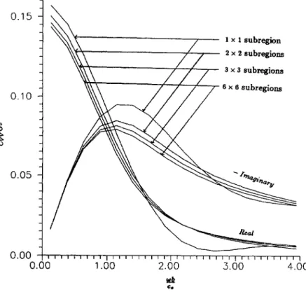
Only a quarter of the plate is used in modelling the system, since the square plate is symmetric with respect to the x- and y-axes. The accuracy of the results is dependent upon how many components are used for the truncated integrand in equation (16) and how fine the meshed contact region in equation (1) is. To address these problems, a numerical scheme is devised for the example. In the scheme, the contact region is always divided into subregions with equal size. Figures 2 and 3 show some of the results. Figure 2 compares the

results by changing the number of subregions for the square contact area. Examining this figure, one can see that the model with 3 x 3 subregions has given fair results for the example. Figure 3 compares results by changing the number of components left in the integrand. It is concluded that all the components of n Q 8 are

needed in order to obtain good results for the example.

Therefore, the 3 x 3 subregion mesh of the square contact region and the truncated integrand of all the components n

<

8 are assigned to the scheme of verification. Figure 4 shows the comparison of the results of the proposed method and that in Reference 7. In the figure, the present results are in fair agreement with the results in Reference 7, except for some 10 per cent disagreement for the imaginary part over the frequency range 07-2-7. However, one can see that the disagreement is becoming smaller as the hysteretic damping ratio

t -,

0. This zero damping condition is presumed in Reference 7. Also, to generate one compliance using the proposed method with a 3 x 3 mesh and n

<

8, the C P U time on a SUN IV work station is less than 2 min.

0.10

?

0"

0.05 0.00 0.00 1

.oo

2.00 3.00 4.00 rrp C .

Figure 2. Vertical compliances of different meshes

(t

= 0.05, n

<

8 )

!d

a.

1124 G.-S. LIOU 0.10

?

6

0.05

0.00

0.00 1

.oo

2.00 3.00 4.00 0.1 5 Reference 7

e

= .02 = .05 € = .10 !& C.

Figure 4. Comparison of vertical compliances (n

<

8, 3 x 3 subregions)

CONCLUDING REMARKS

Based on the procedure developed and the numerical example carried out, the following suggestions can be made.

The shapes of subregions for the piecewise constant traction model in equation (1) can be arbitrary, e.g. rectangular, triangular,

. . .

etc. This will make the contact stress model easier to fit in the arbitrary shapes of foundations.

Although the distribution of the contact stresses is assumed to be piecewise constant, higher order distributions can be used in the proposed method without difficulty. These higher order distributions may reduce the number of subregions needed to attain the precision, and perhaps save some computational cost.

The procedure can be extended easily to the cases of a layered medium. To do this, one just has to replace the matrix Q in equation (16) with the equivalent matrix

of

the layered medium. The equivalent matrix can be obtained using the transfer matrix between layers, as shown in Reference 9.

Examining equation (16), one can observe that most of the computational effort is expended in generating the matrices DS, and D; which are the results of surface integrals. However, these matrices, in

contrast to the counterpart in the boundary element methods of using Green functions or fundamental solutions, are independent of the complexity of the subsoil and the excitation frequency, since the changes of soil properties and excitation frequency are reflected only in the matrix Q of equation (16). This Q matrix is easy to calculate, even for a medium with multiple layers. Therefore, the method

presented should have an advantage over the boundary element methods in calculating the impedance matrix for a surface foundation, if the subsoil consists of many different layers.

5. Furthermore, one also can calculate simultaneously several K matrices of equation (16) with respect to different excitation frequencies, if enough storage space in the computer is reserved for these K matrices. This means that one can generate several impedance matrices with respect to several different excitation frequencies at one time. This is because those matrices DS, and Di in equation (16) and matrix B in

equation (2 1) are independent of the excitation frequency. Actually, the method presented, when compared to the boundary element methods, needs a smaller storage space in a computer. This feature of the method presented would further slash the computational cost of generating a foundation impedance matrix for soil-structure interaction.

ACKNOWLEDGEMENTS

This work is sponsored by National Science Council of Taiwan under Contract No. NSC79-0410-E009-16. The numerical computations are performed in the SUN IV work station at the Department of Civil Engineering, National Chiao-Tung University. These supports are greatly appreciated.

REFERENCES

1. T.-J. Tzong and J. Penzien, ‘Hybrid-modelling of soil-structure interaction in layered media, Report No. UBC/EERC-83/22,

2. F. Chapel, ‘Boundary element method applied to linear soil-structure interaction on a heterogeneous soil’, Earthquake eng. struct.

3. I. A. Robertson, ‘Forced vertical vibration of a rigid circular disk on a semi-infinite elastic solid, Proc. Camb. phil. SOC. 62, 547-553

4. J. E. Luco and R. A. Westman, ‘Dynamic response of circular footings’, J. eng. mech. div. ASCE 97, 1381-1395 (1971).

5. J. Lysmer, ‘Vertical motion of rigid footings’ Contract Report No. 3-115, Department of Civil Engineering University of Michigan, 6. A. S. Veletsos and Y. Tang, ‘Vertical vibration of ring foundations’, Earthquake eng. struct. dyn. 15, 1-21 (1987).

7. H. L. Wong and J. E. Luco, ‘Dynamic response of rigid foundations of arbitrary shape’, Earthquake eng. struct. dyn. 4, 579-587

8. H. L. Wong and J. E. Luco, ‘Tables of impedance functions for square foundations on layered media’, Soil dyn. earthquake eng. 4, 9. G.-S. Liou, ‘Analytical solution for soil-structure interaction in layered media’, Earthquake eng. struct. dyn. 18, 667486 (1989).

10. K. Sezawa, ‘Further studies on Rayleigh waves having some azimuthal distribution’, Bull. earthquake res. inst. Tokyo Llniu. 6, 1-18 Earthquake Engineering Research Center, University of California, Berkeley, CA, 1983.

dyn. 15, 815-829 (1987). (1966).

-

1965. (1976). 6 4 8 1 (1985). (1929).