國 立 交 通 大 學
應用數學系
數學建模與科學計算碩士班
碩
士
論
文
一個對於變動曲面的網格重構之研究
A remeshing study for evolving surfaces
研 究 生:關湘源
指導教授:賴明治 教授
一個對於變動曲面的網格重構之研究
A remeshing study for evolving surfaces
研 究 生:關湘源 Student:Hsiang-Yuan Kuan
指導教授:賴明治 教授 Advisor:Ming-Chih Lai
國 立 交 通 大 學
應用數學系數學建模與科學計算碩士班
碩 士 論 文
A ThesisSubmitted to Department of Applied Mathematics College of Science
Institute of Mathematical Modeling and Scientific Computing National Chiao Tung University
in Partial Fulfillment of the Requirements for the Degree of
Master in
Applied Mathematics September 2013
Hsinchu, Taiwan, Republic of China
一個對於變動曲面的網格重構的研究
學生:關湘源 指導教授:賴明治 教授
國立交通大學應用數學系數學建模與科學計算碩士班
摘 要
我們提出了一個以提高網格質量的理念為基礎的重新網格化方
法,利用一連串區域的運算來改進網格的幾何性質。其核心技術為
Area-based smoothing ,此方法能建造一個非均勻網格,並且能有效
地降低鈍角三角形的數目。
A remehsing study for evolving surfaces
Student : Hsiang-Yuan Kuan Advisor : Ming-Chih Lai
Institute of Mathematical Modeling and Scientific Computing
Department of Applied Mathematics
National Chiao Tung University
ABSTRACT
We present a remeshing scheme based on the idea of improving mesh
quality by a series of local modifications of the mesh geometry and
connectivity. The central local modification technique is an area-based
smoothing technique. Area-based smoothing allows the control of both
triangle quality and vertex sampling over the mesh, as a function of some
criteria, e.g. the mesh curvature. The algorithm is able to create an
unstructured mesh, and reduce irregular vertices efficiently.
誌 謝
首先誠摯的感謝指導教授賴明治教授,老師悉心的教導使我得以
了解應用數學與計算數學的應用,不時的討論並指點我正確的方向,
使我在這些年中獲益匪淺。
兩年多的日子裡,研究室裡共同的生活點滴,學術上的討論、趕
作業的革命情感、一起出遊的回憶…,感謝眾位學長姐、同學、學弟
妹的共同砥礪,你們的陪伴讓兩年的研究生活變得絢麗多彩。
特別感謝陳冠羽、胡偉帆學長們不厭其煩的指出我研究中的缺
失,且總能在我迷惘時為我解惑,也感謝張毓倫同學與我共同討論並
給予意見。
女朋友在背後的默默支持更是我前進的動力,沒有的體諒、包容,
相信這兩年的生活將是很不一樣的光景。
最後,謹以此文獻給我摯愛的雙親,沒有你們就沒有今天的我。
關湘源 謹致於
交通大學數學建模與科學計算所
目 錄
中文提要 ……… i
英文提要 ……… ii
誌謝
……… iii
目錄
……… iv
一、 Introduction
……… 1
二、 Contribution and Overview ……… 2
三、 Surface Reconstruction
……… 2
四、 Remeshing ……… 6
五、 Connectivity Regularization ……… 11
六、 Numerical Results ……… 13
七、 Conclusion……… 20
Reference ……… 21
1
Introduction
Triangular meshes are used to approximate surfaces or flow fields for rendering and simulation. Triangles with large angles are also found to hamper the efficiency of some iterative algebraic solvers. This implies that obtuse triangles should be avoided as much as possible. The control of the maximum angle is difficult, however. Especially for the triangular mesh under flow, it always produce meshes that contain a large number of obtuse triangles. There are a number of methods for generating triangular meshes [3, 10, 11]. However, none of these methods consider avoiding obtuse triangles.
In this paper, we present an effective method for reducing obtuse triangles effi-ciently.
1.1
Related Works
Recent remeshing algorithms, e.g. [2, 6, 9] are based on global parameterization of the original mesh, and then a resampling of the parameter domain. Following this, the new triangulation is projected back into 3D space, resulting in an improved version of the original model. The main drawback of the global parameterization methods is the sensitivity of the result to the specific parameterization used, and to the cut used to force models that are not isomorphic to a disk to be so. Embedding a non-trivial 3D structure in the parameter plane severely distorts this structure, and important information, which is not specified explicitly, may be lost on the way. Even if the parameterization minimizes the metric distortion of the 3D origi-nal in some reasonable sense, it is impossible to eliminate it completely. Moreover, methods finding a global parameterization are slow, usually involving the solution of a large set of (sometimes nonlinear) equations. Recent progress may accelerate the process to almost linear time even for large meshes, using multi-resolutional approaches, e.g. [15], inspired by multi-grid methods together with good precondi-tioning. Unfortunately, when dealing with extremely large meshes, or meshes with severe isoperimetric distortion (like sock-shaped regions) numerical precision issues may arise. In such cases, a global parameterization is almost impossible to perform without using multi-scale or precise arithmetic representation of the parametric do-main.
The main alternative to global parameterization is to work directly on the surface and perform a series of local modifications on the mesh. This approach is also known as the mesh adaptation process and is the one we use in this work. Remeshing algorithms using this approach [1, 5, 7, 8, 14, 19] usually involve computationally expensive optimizations in 3D or more efficient but less accurate optimization in the tangent plane. In Section 3.2, we use PN triangles as a good tradeoff between accuracy and efficiency.
2
Contribution and Overview
In this paper we present a remeshing method which we call explicit. The word explicit we mean that we operate directly on the mesh surface and apply local modifications to it, instead of working on some indirect representation of the surface, e.g. on a global parametric domain. The components of our remeshing algorithm are natural and straightforward ways to improve a mesh. Our scheme is based on the work that Vitaly Surazhsky and Craig Gostman presented [17]. We use local parameterization to reduce the problem of local mesh optimizations to 2D.
Our remeshing algorithm incorporates a number of novel techniques, each of independent interest. The central technique is the area-based mesh optimization described in Section 4, which manipulates the areas of triangulation in order to achieve a uniform or otherwise specified vertex sampling. Section 5 presents a novel regularization technique that performs local modifications to the mesh connectiv-ity, resulting in a mesh whose connectivity is much regular. When combined, our techniques provide an accurate and robust remeshing algorithm that can be applied to meshs of arbitrary genus. Our remeshing scheme is very efficient and is easy to coding.
3
Surface Reconstruction
We perform an estimate of the smooth surface in the vicinity of a mesh tri-angle. This may be obtained by reconstructing an approximation of the surface using triangular cubic B´ezier patches for every face of the mesh. Vlachos et al. [20] presented a simple and efficient yet robust and accurate method to construct such curved patches called P N triangles.The triangle vertex normals together with vertex coordinates are used to construct a PN triangle. If the normals at the mesh vertices are not given, we use a method similar to [13] to define them, and we will introduce the algorithm later. The normal of any point within a PN triangle is defined as an efficient quadratic interpolation of the normals at the triangle vertices. We use PN triangles as a good tradeoff between accuracy and efficiency.
3.1
Normals
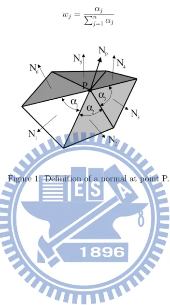
The definition of cubic B´ezier triangle requires normals to be provided or ap-proximated at each vertices. Defining the normal, NP at a point as the weighted
average of the adjacent faces normal, Nj, where the weight, wj is the normalized
angle at the point. Equations (1), (2) and Figure 1 describe this procedure. NP =
n
X
j=1
wj =
αj
Pn
j=1αj
(2)
3.2
PN triangle
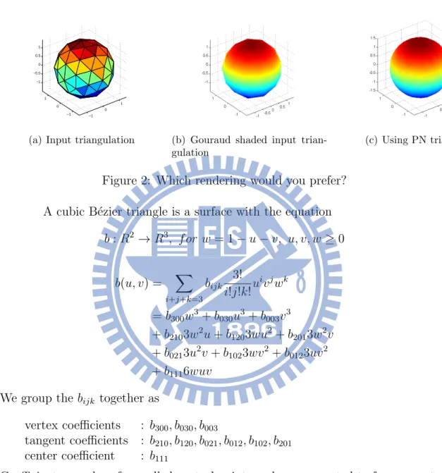
−1 0 1 −1 0 1 −1 −0.5 0 0.5 1(a) Input triangulation (b) Gouraud shaded input trian-gulation
(c) Using PN triangles
Figure 2: Which rendering would you prefer? A cubic B´ezier triangle is a surface with the equation
b : R2 → R3, f or w = 1 − u − v, u, v, w ≥ 0 b(u, v) = X i+j+k=3 bijk 3! i!j!k!u i vjwk = b300w3+ b030u3+ b003v3 + b2103w2u + b1203wu2+ b2013w2v + b0213u2v + b1023wv2+ b0123uv2 + b1116wuv
We group the bijk together as
vertex coefficients : b300, b030, b003
tangent coefficients : b210, b120, b021, b012, b102, b201
center coefficient : b111
Coefficients are also often called control points and are connected to form a control net(see Figure 3(b)).
We are given the positions P1, P2, P3 ∈ R3 and normal N1, N2, N3 ∈ R3 of the
tri-angle corners as shown in Figure 3(a). In formulas for implementation, coefficients of the PN triangle are defined as follows:
b300 = P1,
b030 = P2,
b003 = P3,
b210 = (2P1+ P2− w12N1)/3, b120 = (2P2+ P1− w21N2)/3, b021 = (2P2+ P3− w23N2)/3, b012 = (2P3+ P2− w32N3)/3, b102 = (2P3+ P1− w31N3)/3, b201 = (2P1+ P3− w13N1)/3, E = (b210+ b120+ b021+ b012+ b102+ b201)/6, V = (P1+ P2+ P3)/3, b111 = E + (E − V )/2.
(a) Input date: points Pi and normals Ni
(b) The coefficients or control points of a triangular B´ezier patch arranged to form a control net
4
Remeshing
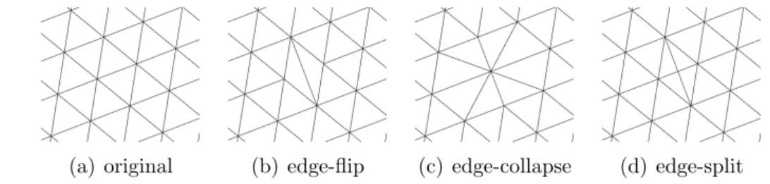
(a) original (b) edge-flip (c) edge-collapse (d) edge-split
Figure 4: Types of edge operation
The focus of our remeshing scheme is on maximizing the angles of all tri-angles of the mesh. Remeshing of the given mesh M is performed by a series of local modifications. The most well-known and commonly used local modifications are edge − f lip, edge − collapse, edge − split and vertex relocation.
The main stages of our remeshing scheme are as follows: • Adjust the number of vertices of M
• Apply the area-based remeshing procedure on M • Regularize M using the algorithm of Section 5 • Apply the angle-based smoothing procedure on M
collapse and edge-split are used to change the number of mesh vertices. Edge-flip and vertex relocation improve the quality of the mesh triangles. The area-based remeshing procedure is the heart of our remeshing scheme and produces a mesh with high quality triangles and the required vertex sampling. Another two stages improve the mesh quality further. The regularization stage improves the regularity of the mesh connectivity. The angle-based smoothing then polishes the mesh to obtain the optimal mesh geometry without changing its connectivity.
The area-based remeshing and the angle-based smoothing involve the most crit-ical and difficult operation − vertex relocation.
4.1
Vertex Relocation
Let v be a vertex having location x(v) and whose neighbors are v1, · · · , vk with
locations x(v1), · · · , x(vk), respectively, and k is the vertex degree. We want to find
a new location xnew(v) satisfying some condition, e.g. improving the angles of the
triangles incident on v. A solution to this problem that directly finds xnew(v) in 3D
usually involves solving a difficult optimization problem, which may have non-linear constraints. We overcome this problem by mapping faces incident on v into the 2D
−3 −2.9 −2.8 −2.7 −2.6 −1.2 −1 −0.8 −0.9 −0.8 −0.7 −0.6 v4 v5 v6 v3 v v2 v1 (a) S(v) −0.5 −0.4 −0.3 −0.2 −0.1 0 0.1 0.2 0.3 0.4 −0.4 −0.3 −0.2 −0.1 0 0.1 0.2 0.3 p p1 p2 p3 p4 p5 p6 pnew (b) SP(v)
Figure 5: Vertex relocation
plane and solving the problem there. The location computed in the plane is then brought back to the original surface.
Let S(v) be a sub-mesh of M containing only v, v1, · · · , vk and faces incident on
v. (See Figure 5(a)) We map S(v) into the plane using a natural and simple method approximating the geodesic polar map [16], as described, for example, by Welch and Witkin [21] and Floater [4]. Let p, p1, · · · , pk be the positions of vertices v, v1, · · · , vk
within the resulting mapping SP(v). p is mapped to the origin. p1, · · · , pk satisfy
the following conditions: the distances between p and its neighbors are the same as the corresponding distances in M , namely, kp − pik = kx(v) − x(vi)k for 1 ≤ i ≤ k.
The angles of all triangles at p are proportional to the corresponding angles in M and sum to 2π.
The next step is to find a new location pnew to satisfies some condition, we will
introduce it later. (See Figure 5(b))
4.2
Back to the Original Surface
After the new vertex location pnew has been found, we need to find its
corre-sponding location on the original surface, namely, to find xnew(v). Existing
remesh-ing methods, e.g. [1, 8, 14] solve this problem by findremesh-ing the vertex projection onto the original surface. Projecting the vertex involves a computationally expensive and not always accurate computation that without special care may even lead to topological errors during the remeshing process.
In our case, xnew(v) is computed by a barycentric coordinate scheme. Given a
point p and that the triangle (q1, q2, q3) contains p, we can compute its barycentric
coordinate b0 = (b1, b2, b3) using (3). Then we apply the method PN triangle in
Section 3.2 to find it.
b1 = A(p, q2, q3) A(q1, q2, q3) , b2 = A(p, q3, q1) A(q1, q2, q3) , b3 = A(p, q1, q2) A(q1, q2, q3) (3)
where A(qi, qj, qk) is the signed area of triangle (i, j, k).
4.3
Area-based Remeshing
The concept of triangle areas has never been used as a central factor in mesh generation. Triangle areas are usually used to assist, analyze or control meshing. The reason for this is that by using triangle areas alone we cannot obtain meshes of reasonable quality. A mesh optimization that equalizes the areas of the mesh triangles or brings triangle areas to specified (absolute or relative) values will, in most cases, result in many long and skinny triangles. Nevertheless, Surazhsky and Gotsman [18] discovered that a 2D triangulation having triangles with equal (or close to equal) areas has globally uniform spatial vertex sampling. They presented the following remeshing scheme that exploits this: Alternate between area equalization and a series of angle-improving (Delaunay) edge-flips. Applying this simple scheme results in a 2D mesh with a very uniform sampling and well-shaped triangles.
It is important to mention that this alternation process does not usually converge. After a uniform sampling rate is obtained, the process begins to oscillate, producing different but similar uniform vertex distributions. However, this oscillation is not a problem for our remeshing algorithm, since subsequent steps of our remeshing algorithm improve quality of the mesh further by regularizing and smoothing it.
4.4
Area-based Vertex Relocation
Area equalization is done iteratively by relocating every vertex such that the areas of the triangles incident on the vertex are as equal as possible. In this work we extend this method to relocating vertices such that the ratios between the areas are as close as possible to some specified values. To define this formally, we return to the definitions of point p and its neighbors p1, · · · , pk from Section 4.1. Let (xi, yi)
be the coordinates of pi. Our goal is to find p = (x, y) such that the ratios of the
triangle areas are as close as possible to µ1, · · · , µk. µi is all positive and sum to
unity. Denote Ai(x, y) be the area of triangle p, pi, pi+1:
Ai(x, y) = 1 2 xi yi 1 xi+1 yi+1 1 x y 1
Let A be the area of polygon (p1, · · · , pk), which may be computed asPki=1Ai(0, 0).
Now the location of p is defined as follows: (x, y) = arg min (x,y) k X i=1 (Ai(x, y) − µiA)2
This reduces to solving a system of two linear equations in x and y, which has a unique solution. Thus, area-based relocation is almost as efficient as Laplacian smoothing.
4.5
Curvature Sensitive Remeshing
We now show how to use area-based vertex relocation to produce a mesh re-flecting the curvature of the original mesh. Intuitively, more curved regions of M will contain small triangles and a dense vertex sampling, while almost flat regions will have large triangles with more sparse vertices. The idea is to specify ratios between triangle areas depending on curvature.
Let Ψ be a density function defined over M . For every vertex v of M , we define Ψ(v) as 1/(α|K(v)| + βH2(v)), where H(v) and K(v) are approximated discrete
Gaussian and mean curvatures, respectively. α and β are user-defined values, which are positive and sum to unity. Usually we use α = β = 0.5. We compute H(v) and K(v) using the method described in [12].
The next step is to define the triangle area ratios that we use in vertex relocation. We return to the notations of Section 4.4. Define µ0i for 1 ≤ i ≤ k as the average between Ψ(vi) and Ψ(vi+1). The value µ0i describes the required density of the
corresponding triangle (v, vi, vi+1). Then µ01, · · · , µ 0
k are normalized to obtain valid
µ1, · · · , µk, namely, µi = µ0i/ Pk j=1µ 0 j
4.6
Weight-angle-based smoothing
Zhou and Shimada [22] presented an effective and easy to implement based mesh smoothing scheme. They show that the quality of the mesh after angle-based smoothing is much better than after Laplacian smoothing. Moreover, the chance that the scheme will produce inverted (invalid) faces is much less than that in Laplacian smoothing. Unfortunately, this is true mostly for meshes whose vertices have degrees close to the average degree, namely, the mesh connectivity is close to regular. When the mesh has more irregular connectivity, the scheme may fail. In applications involving meshes with very distorted (long and skinny) triangles, a more robust smoothing scheme is critical. We propose a very simple improvement to the original angle-smoothing scheme, which significantly reduces the chances of inverted triangles and improves the quality of the resulting mesh. Furthermore, it has almost the same computational cost per iteration and a lower total computational cost due to better convergence in practice.
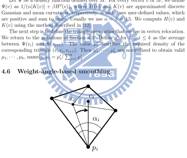
The original scheme attempts to make each pair of adjacent angles equal. Given a vertex c and its neighbours p1, · · · , pk, we want to move c in order to improve
the angles of the triangles incident on c. Let αi be the angle adjacent to pi in the
polygon p1, · · · , pk. We define ci to be the point lying on the bisector of αi such that
kpi− cik = kpi− ck, namely, the edge (pi, c) is rotated around pi to coincide with
the bisector of αi(see Figure 4). The new position of c is defined as the average of
all ci for all the neighbours, namely:
cnew = 1 k k X i=1 ci (4)
We improve this scheme by introducing weights into Eq.4. For a small angle αi
it is difficult to guarantee that the resulting cnew will be placed relatively close to
the bisector of αi. Since αi is itself small, a large deviation of cnew from the bisector
of αi will create angles not only much smaller than αi/2 but even negative (invalid)
ones. Thus, the resulting mesh will have poor quality. To prevent this, we modify Eq.4 in the following way:
cnew= 1 Pk i=11/α2i · k X i=1 1 α2 i · ci
Namely, the ci for small angles αi will carry more weight than for large angles.
4.7
Implementation Notes
Area-based remeshing
The procedure is controlled by two parameters: nstep and narea. We alternate
nsteptimes times between curvature sensitive area equalization and a series of
vertex relocation for every vertex of M . Edge-flips are performed until a Delaunay edge-flip can no longer be applied. nstep and narea are usually small. There is no
need to bring the triangle areas as close as possible to some required ratios to change vertex sampling. A very small number (1 to 3) of narea iterations is enough to move
vertices in the proper direction towards the required vertex sampling. nstep is
usu-ally between 5 and 10 and is sufficient to produce a mesh with vertex sampling very close to the required one.
Angle-based smoothing
The parameter mstep of this procedure defines how many iterations of weighted
angle-based smoothing are performed. Each iteration relocates once every vertex of M . mstep is also small and usually somewhere between 5 and 10.
Adjusting the number of the mesh vertices
To obtain a mesh with the number of vertices specified by the user, we apply local refinement or simplification operations to the mesh. Until the required number of vertices is achieved we perform a series of edge-collapse or edge-split modifications (depending on the required size) such that the edges affected by the modifications are an independent edge set. Edges whose faces have minimal/maximal angle are simplified/refined first. Before every series of modifications we apply the area-based remeshing procedure with nstep=1 to maintain a fair vertex sampling.
5
Connectivity Regularization
Another component of our remeshing scheme is an effective yet simple and efficient algorithm to improve the mesh quality by regularizing its connectivity. The algorithm performs a series of local operations that modify the mesh connectivity, namely, edge-flips, edge-collapses and edge-splits. Formally, improving regularity means minimizing the following function:
R(M ) = X
v∈M
(d(v) − dopt(v))2
where d(v) is the degree of vertex v and dopt(v) its optimal degree, which is equal to
6. We do not define this formally, but during the mesh regularization we allow only a small change in the total number of mesh vertices and vertex sampling along the mesh.
We call an edge-flip basic if it decreases R(M ). In their elegant work, Alliez et al. [2] proposed to randomly apply basic edge-flips to regularize mesh connectivity. This straightforward method results in some improvement. However, it still leaves
too many irregular vertices even when basic edge-flips can no longer be applied. The reason for this is that R has many local minima with respect to basic edge-flips. The intriguing question is how to continue from such a local minimum.
We pose this problem as a puzzle. The player can click an edge to flip, collapse or split it. We call an edge easy if we can apply a basic edge-flip on it. The game starts with a mesh without easy edges, namely, when R(M ) is at a local minimum. The goal of the game is to minimize R(M ) further with a small number of mesh modifications. To visualize, we color vertices according to their degree. A vertex v is black if d(v) < dopt(v) and white when d(v) > dopt(v). The vertex is not colored
when d(v) = dopt(v), namely, the player has solved the puzzle for v. See Figure 7.
When solving the puzzle we discovered that there are three types of edges that are actually interesting, and for every type there is only one specific local modification to apply.
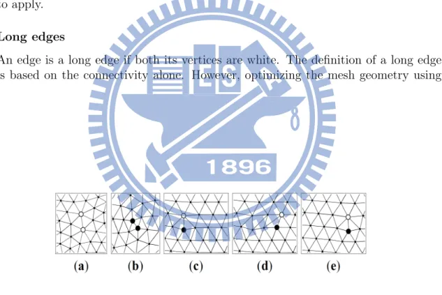
Long edges
An edge is a long edge if both its vertices are white. The definition of a long edge is based on the connectivity alone. However, optimizing the mesh geometry using
Figure 7: Types of edges: (a) A long edge. (b) A short edge. (c) A drifting edge. (d) The drifting edge moved two steps to the right. (e) After angle-based smoothing.
the angle-based smoothing reveals that long edges are actually geometrically longer than their nearby edges. Thus, the natural modification for this edge is to refine it. See Figure 5(a).
Short edges
An edge is a short edge if both of its vertices are black. Short edges are actually shorter than other nearby edges if the mesh has been optimized using the anglebased smoothing procedure. Thus, we collapse short edges. See Figure 5(b).
Drifting edges
An edge is a drifting edge if one of its endpoints is a white vertex and the other is black. Every drifting edge e has the following nice property: If we flip an edge e0 incident on the white vertex that belongs to one of the faces adjacent to e, then e disappears (loses its drifting property) and reappears as the opposite to e within the quad defined by e0. Thus, we say that we have moved a drifting edge. This allows us to move a pair of white and black vertices of a drifting edge across a regular region of the mesh; see Figure 5(c-e).
5.1
Solving the Puzzle
To every edge among long, short or drifting edges, we apply only its correspond-ing operation. The central idea in solvcorrespond-ing the puzzle is to cause a driftcorrespond-ing edge to migrate until it meets irregular vertices, and thus, an easy, long or short edge may appear. We perform operations on these edges, until only drifting edges are left. Then we choose an arbitrary drifting edge as the next edge to move.We proceed this way, until no drifting edge is left. This condition means that there are no easy, long and short edges as well, and the algorithm terminates. Consequently, the algorithm results in a mesh that has all irregular vertices surrounded by regular vertices. The number of such isolated irregular vertices is usually very small.
6
Numerical Results
First, we will show the remeshing method can reduce obtuse triangle and im-prove the angle in the mesh. Second, we compute the mean curvature on the original mesh, mesh after remesh, and after mesh refinement, to show that both of them are more accurate than the original mesh.
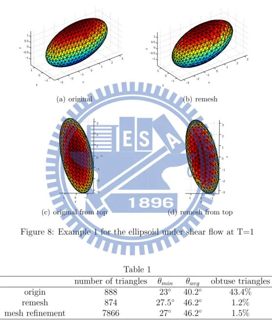
1
Example 1 −3 −2 −1 0 1 2 3 −1 0 1 −1 −0.5 0 0.5 1 x y z (a) original −3 −2 −1 0 1 2 3 −1 0 1 −1 −0.5 0 0.5 1 x y z (b) remesh −3 −2 −1 0 1 2 3 −1 0 1 x y(c) original from top
−3 −2 −1 0 1 2 3 −1 0 1 x y
(d) remesh from top
Figure 8: Example 1 for the ellipsoid under shear flow at T=1
Table 1
number of triangles θmin θavg obtuse triangles
origin 888 23◦ 40.2◦ 43.4% remesh 874 27.5◦ 46.2◦ 1.2% mesh refinement 7866 27◦ 46.2◦ 1.5%
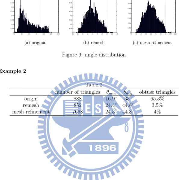
20 40 60 80 100 120 140 0 0.005 0.01 0.015 0.02 0.025 0.03 0.035 0.04 (a) original 20 30 40 50 60 70 80 90 100 110 0 0.005 0.01 0.015 0.02 0.025 0.03 0.035 0.04 (b) remesh 20 30 40 50 60 70 80 90 100 110 0 0.005 0.01 0.015 0.02 0.025 0.03 0.035 (c) mesh refinement
Figure 9: angle distribution Example 2
Table 2
number of triangles θmin θavg obtuse triangles
origin 888 16.9◦ 33◦ 65.3% remesh 852 24.4◦ 44.8◦ 3.5% mesh refinement 7668 24.3◦ 44.8◦ 4%
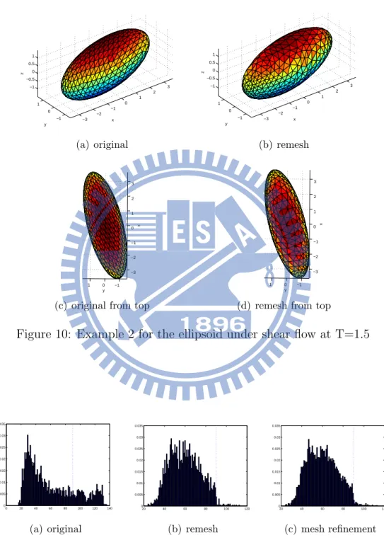
−3 −2 −1 0 1 2 3 −1 0 1 −1 −0.5 0 0.5 1 x y z (a) original −3 −2 −1 0 1 2 3 −1 0 1 −1 −0.5 0 0.5 1 x y z (b) remesh −3 −2 −1 0 1 2 3 −1 0 1 x y
(c) original from top
−3 −2 −1 0 1 2 3 −1 0 1 x y
(d) remesh from top
Figure 10: Example 2 for the ellipsoid under shear flow at T=1.5
0 20 40 60 80 100 120 140 0 0.005 0.01 0.015 0.02 0.025 0.03 0.035 (a) original 20 40 60 80 100 120 0 0.005 0.01 0.015 0.02 0.025 0.03 0.035 (b) remesh 20 40 60 80 100 120 0 0.005 0.01 0.015 0.02 0.025 0.03 0.035 (c) mesh refinement
−2 −1 0 1 2 −1 0 1 −1 −0.5 0 0.5 1 x y z (a) T=0 −2.5 −2 −1.5 −1 −0.5 0 0.5 1 1.5 2 2.5 −1 0 1 x y (b) top −3 −2 −1 0 1 2 3 −1 0 1 −1 −0.5 0 0.5 1 x y z (c) T=0.5 −3 −2 −1 0 1 2 3 −1 0 1 x y (d) top −3 −2 −1 0 1 2 3 −1 0 1 −1 −0.5 0 0.5 1 x y z (e) T=1 −3 −2 −1 0 1 2 3 −1 0 1 x y (f) top −3 −2 −1 0 1 2 3 −1 0 1 −1 −0.5 0 0.5 1 x y z (g) T=1.5 −3 −2 −1 0 1 2 3 −1 0 1 x y (h) top
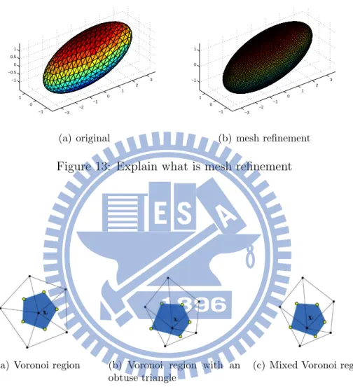
−3 −2 −1 0 1 2 3 −1 0 1 −1 −0.5 0 0.5 1 (a) original −3 −2 −1 0 1 2 3 −1 0 1 −1 0 1 (b) mesh refinement
Figure 13: Explain what is mesh refinement
(a) Voronoi region (b) Voronoi region with an obtuse triangle
(c) Mixed Voronoi region
(d) 1-ring neighbors and an-gles opposite to an edge
2
To compute the mean curvature numerically, we have already known that the equation ∆sX = 2Hn, where H is the mean curvature and n is the outward unit
normal. The mean curvature is defined on the vertex of triangle: ∆sXi = 1 AM(Xi) X j∈N1(Xi) cot αij + cot βij 2 (Xi − Xj)
The N1(Xi) means the 1-ring neighbors of vertex Xi, AM(Xi) is the area of Mixed
Voronoi region (see Figure 14). The angles αij and βij are shown in Figure 14(d).
To measure the error, we compute the maximum error in the notation k · k∞ by
max |H(xi) − Hexact| and the average error byP |H(xi) − Hexact|/N , where N is the
number of vertices. Original mesh x2 32 + y2 1.52 + z2 1.52 = 1
k · k∞ average error number of obtuse triangles
h=0.5 0.4633 0.0100 2/408 h=0.25 0.0232 0.0031 0/2072 h=0.125 0.0153 0.0025 1/8760 h=0.0625 0.0179 0.0023 0/35832 Under flow
Evolving under shear flow u = (y, 0, 0) with h = 0.25
k · k∞ average error number of obtuse triangles
t=0 0.0232 0.0031 0/2072 t=0.5 0.1384 0.0069 112/2072
t=1 0.4807 0.1027 984/2072 t=1.5 0.8136 0.2491 1461/2072 Remesh for t=1
k · k∞ average error number of obtuse triangles
origin 0.4807 0.1027 984/2072 remesh 0.3032 0.0141 70/2024 mesh refinement 0.3856 0.0080 293/8096
(a) original (b) remesh (c) mesh refinement
Figure 15: mean curvature for t=1 Remesh for t=1.5
k · k∞ average error number of obtuse triangles
origin 0.8136 0.2491 1461/2072 remesh 0.3468 0.0163 52/2024 mesh refinement 0.6159 0.0078 297/8048
(a) original (b) remesh (c) mesh refinement
Figure 16: mean curvature for t=1.5
7
Conclusion
Our method can greatly reduce the number of obtuse triangles in the given triangular mesh. However, it still cannot remove obtuse triangles completely. The reason is the regularity. In Section 5, we improve the mesh quality by regularizing its connectivity, but it still exists irregular vertices. The irregular vertices usually generate obtuse triangles. Hence, further research is needed to improve the result of the regularity.
Reference
[1] J. M. Savignat O. Stab. A. Rassineux, P. Villon. Surface remeshing by local hermite diffuse interpolation. International Journal for Numerical Methods in Engineering, 49:31–49, 2000.
[2] Pierre Alliez, Mark Meyer, and Mathieu Desbrun. Interactive geometry remesh-ing. In Proceedings of the 29th annual conference on Computer graphics and interactive techniques, SIGGRAPH ’02, pages 347–354, 2002.
[3] Siu-Wing Cheng, Tamal K. Dey, Edgar A. Ramos, and Rephael Wenger. Anisotropic surface meshing. In Proceedings of the seventeenth annual ACM-SIAM symposium on Discrete algorithm, SODA ’06, pages 202–211, 2006. [4] Michael S. Floater. Parametrization and smooth approximation of surface
tri-angulations. Comput. Aided Geom. Des., 14(3):231–250, 1997.
[5] Pascal J. Frey. About surface remeshing. In IMR, pages 123–136, 2000.
[6] Xianfeng Gu, Steven J. Gortler, and Hugues Hoppe. Geometry images. In Proceedings of the 29th annual conference on Computer graphics and interactive techniques, SIGGRAPH ’02, pages 355–361, 2002.
[7] Hugues Hoppe. Progressive meshes. In Proceedings of the 23rd annual confer-ence on Computer graphics and interactive techniques, SIGGRAPH ’96, pages 99–108, 1996.
[8] Hugues Hoppe, Tony DeRose, Tom Duchamp, John McDonald, and Werner Stuetzle. Mesh optimization. In Proceedings of the 20th annual conference on Computer graphics and interactive techniques, SIGGRAPH ’93, pages 19–26, 1993.
[9] Kai Hormann, Ulf Labsik, and G¨unther Greiner. Remeshing triangulated sur-faces with optimal parameterizations. Computer-Aided Design, 33(11):779–788, 2001.
[10] Francois Labelle and Jonathan Richard Shewchuk. Anisotropic voronoi dia-grams and guaranteed-quality anisotropic mesh generation. In Proceedings of the nineteenth annual symposium on Computational geometry, SCG ’03, pages 191–200, 2003.
[11] Greg Leibon and David Letscher. Delaunay triangulations and voronoi diagrams for riemannian manifolds. In Proceedings of the sixteenth annual symposium on Computational geometry, SCG ’00, pages 341–349, 2000.
[12] Mark Meyer, Mathieu Desbrun, Peter Schr¨oder, and Alan H. Barr. Discrete differential-geometry operators for triangulated 2-manifolds. In Proc. VisMath, pages 35–57. 2002.
[13] Steven J. Owen, David R. White, and Timothy J. Tautges. Facet-based surfaces for 3d mesh generation. In IMR, pages 297–311, 2002.
[14] Houman Borouchaki Pascal J. Frey. Geometric surface mesh optimization. Computing and Visualization in Science, 1:113–121, 1998.
[15] Pedro V. Sander, Steven J. Gortler, John Snyder, and Hugues Hoppe. Signal-specialized parametrization. In Proceedings of the 13th Eurographics workshop on Rendering, EGRW ’02, pages 87–98, 2002.
[16] D.J. Struik. Lectures on Classical Differential Geometry: Second Edition. Addison-Wesley series in mathematics. Addison-Wesley Publishing Company, 1961.
[17] Vitaly Surazhsky and Craig Gotsman. Explicit surface remeshing. In Pro-ceedings of the 2003 Eurographics/ACM SIGGRAPH symposium on Geometry processing, SGP ’03, pages 20–30, 2003.
[18] Vitaly Surazhsky and Craig Gotsman. High quality compatible triangulations. Eng. with Comput., 20(2):147–156, 2004.
[19] Greg Turk. Re-tiling polygonal surfaces. In Proceedings of the 19th annual conference on Computer graphics and interactive techniques, SIGGRAPH ’92, pages 55–64, 1992.
[20] Alex Vlachos, J¨org Peters, Chas Boyd, and Jason L. Mitchell. Curved PN triangles. In Proceedings of the 2001 symposium on Interactive 3D graphics, I3D ’01, pages 159–166, 2001.
[21] William Welch and Andrew Witkin. Free-form shape design using triangulated surfaces. In Proceedings of the 21st annual conference on Computer graphics and interactive techniques, SIGGRAPH ’94, pages 247–256, 1994.
[22] Tian Zhou and Kenji Shimada. An angle-based approach to two-dimensional mesh smoothing. In IMR, pages 373–384, 2000.