考慮整體保單組合之最適自然避險策略 - 政大學術集成

全文

(1)國立政治大學風險管理與保險學研究所碩士論文. 考慮整體保單組合之最適自然避險策略. 政治大. 立 An Optimal Strategy of Natural Hedging for a. ‧ 國. 學. General Portfolio of Insurance Companies. ‧. n. er. io. sit. y. Nat. al. Ch. i n U. v. e n g c h i 博士指導老師：黃泓智研究生: 洪德全撰. 中華民國九十九年六月.

(2) 中文大綱隨著醫療技術進步、環境衛生改善與人類追求健康生活的趨勢，全世界人類的死亡率不斷地下降。在死亡率不斷的改善的情形下，保險公司可能在壽險商品上獲利，但在年金部份卻會因長壽風險而有所虧損。自然避險則是保險公司可行的避險策略之一，即透過公司整體保單的組合，來達到規避死亡率風險和利率風險。此外，不同於之前的相關研究，我們所使用的資料，是由臺灣所有的保險公司提供的經驗死亡率，而不是國民生命表。目前保險公司在定價年金和壽險商品時，使用的死亡率是國民生命表，即假設買年金. 政治大. 商品的被保險人和買壽險商品的被保險人的死亡率是相同的。但是從經驗死亡率. 立. 的資料，我們發現購買年金商品的被保險人，其死亡率會低於買壽險商品的被保. ‧ 國. 學. 險人的死亡率。上述情形，會造成保險商品定價有誤;因此，我們考慮不同性別的年金、壽險的死亡率，並研究這些死亡率之間隨機變動項的相關性，以期在未. ‧. 來死亡率和利率變動下，可以藉由死亡率間的相關性，而抵消總價值變動的變異. sit. y. Nat. 數和定價差異。. n. al. er. io. 根據經驗資料，我們提出一個模型，可透過調整賣出年金和壽險的比例(年. i n U. v. 齡、性別)，使得保險公司能夠針對公司整體保單組合，找到並有效地運用的自. Ch. engchi. 然避險策略。文中最後進行模型敏感度分析，以及提出可能採用的保險商品配置策略，可作為目前保險公司進行死亡率和利率避險的參考。. 關鍵字: 長壽風險、自然避險.

(3) ABSTRACT The mortality rate of human being has decreased year by year due to the improvement of medical and hygienic techniques. With the mortality improvement over time, life insurers may gain a profit and annuity insurers may suffer losses because of longevity risk. However, natural hedging is a feasible strategy to hedge mortality risk and interest risk at the same time. In this paper, we investigate the natural hedging strategy and try to find an optimal collocation of insurance products to deal with longevity risks for. 政治大. the insurance companies. Different from previous literatures, we use the experienced. 立. mortality rates from life insurance companies rather than population mortality rates.. ‧ 國. 學. This experienced mortality data set includes more than 50,000,000 policies which are collected from the incidence data of the whole Taiwan life insurance companies. In. ‧. general, insurance companies use population mortality rates to price life insurance and. y. Nat. sit. annuity products. Nevertheless, the mortality rate of annuity purchasers is averagely. n. al. er. io. lower than that of life insurance purchasers. This situation leads to mispricing. i n U. v. problem of both life insurance and annuity products. So in this paper, we can. Ch. engchi. construct four mortality tables (gender, product) and investigate the correlation of these stochastic variation terms of four mortality rates. According to the correlation relation between these four mortality rates, we can offset the variance of portfolio’s change and difference of mispricing. On the basis of the experienced mortality rates, we demonstrate that the proposed model can lead to an optimal collocation of insurance products and effectively apply the natural hedging strategy to a more general portfolio for life insurance companies.. Keyword: longevity risk, natural hedging.

(4) Table of Contents 1. Introduction and Motivation....................................................... 1 1.1 Agenda ................................................................................. 3 2. Model Setting ............................................................................ 4 2.1 Mortality Rate Model ........................................................... 4 2.2 Interest Rate Model .............................................................. 6. 政治大. 2.3 General Portfolio Model ...................................................... 8. 立. 3. Data .......................................................................................... 11. ‧ 國. 學. 3.1 Mortality Rate Data ........................................................... 11. ‧. Nat. y. 3.2 Interest Rate Data .............................................................. 14. er. io. sit. 4. Numerical Analysis ................................................................... 15 4.1 Scenario 1 : θ =a0 .............................................................. 15. n. iv l C n hengchi U 4.2 Scenario 2 : θ = 1 .............................................................. 21 4.3 Scenario 3 : 0 < θ < 1 ........................................................ 24 4.4 General Portfolio of Insurance Products ............................ 29. 5. Conclusion and Suggestion ....................................................... 33 6. Reference .................................................................................. 35.

(5) Table Catalogue Table 1: Standard deviation of kt in four different products............................ 12 Table 2: Optimal units of life insurances with different  (θ = 0) ................. 15 Table 3: Effective duration and convexity with different  ............................ 16 Table 4: Optimal units of life insurances, given 1 unit of female annuity (θ = 0)16 Table 5: Optimal units of life insurances, given 1 unit of male annuity (θ = 0) 17 Table 6: Effective duration and mortality rate of each product (insured).......... 19. 政治大 Table 8: Comparison of deferred effect of male annuity (θ = 0) ...................... 20 立. Table 7: Comparison of deferred effect of female annuity (θ = 0) ................... 19. ‧ 國. 學. Table 9: Optimal units of annuity, given 1 unit of ml 30 (θ = 0) ...................... 21 Table 10: Optimal units of annuity, given 1 unit of ml 60 (θ = 0) .................... 21. ‧. Table 11: Pricing differences between period and cohort bases ....................... 22. sit. y. Nat. Table 12: Optimal units of life insurances, given 1 unit of annuity (θ = 1)....... 23. io. al. er. Table 13: Comparison of gender effect of annuity (θ = 1) ............................... 23 Table 14: Comparison of age effect of annuity (θ = 1) .................................... 23. n. v i n Cofh female life insurance Table 15: Testing θ: optimal units e n g c h i U .............................24 Table 16: Testing θ: optimal units of male life insurance ................................ 26 Table 17: Optimal units of life insurance, given 1 unit of female annuity........ 27 Table 18: Optimal units of life insurance, given 1 unit of male annuity ........... 27 Table 19: Comparison of age effect of female annuity (θ = 0.001) .................. 28 Table 20: Comparison of age effect of male annuity (θ = 1) ............................ 28 Table 21: Historic allocated amounts in 2007.................................................. 29 Table 22: Small proportional adjustment of historic data ................................ 30 Table 23: Fixed proportions of annuities ......................................................... 32.

(6) Figure Catalogue Figure 1: Parameter Estimates of  x in LC model ........................................ 12 Figure 2: Parameter Estimates of  x in LC model ........................................ 12 Figure 3: Parameter Estimates of kt in LC model ........................................... 12 Figure 4: Forecast of future interest rate of CIR model ................................... 14 Figure 5: Pricing differences between period and cohort bases........................ 23 Figure 6: Testing θ (fa60 vs fl) ........................................................................ 24. 政治大 Figure 8: Optimal pattern of different θ (fa60 vs fl) ........................................ 25 立. Figure 7: Testing θ (ma60 vs fl) ...................................................................... 24. ‧ 國. 學. Figure 9: Optimal pattern of different θ (ma60 vs fl) ....................................... 25 Figure 10: Testing θ (fa60 vs ml) .................................................................... 26. ‧. Figure 11: Testing θ (ma60 vs ml) .................................................................. 26. sit. y. Nat. Figure 12: Optimal pattern of different θ (fa60 vs ml) ..................................... 27. io. al. er. Figure 13: Optimal pattern of different θ (ma60 vs ml) ................................... 27 Figure 14: Optimal units of fl, given 1 unit of different annuities .................... 28. n. v i n Figure 15: Optimal units of ml, C given h e1 unit h i Uannuities ..................28 n gofcdifferent. Figure 16: Optimal pattern under the allowable 15% adjustment level (fa) ..... 31 Figure 17: Optimal pattern under the allowable 15% adjustment level (ma) .... 31 Figure 18: Optimal pattern under the fixed proportions of annuities................ 32.

(7) 1. Introduction and Motivation According to the publication-Sigma of Swiss Re, the life expectancy of human around the world will increase 0.2 year per year. Because the mortality rate has improved rapidly for the past decades, longevity risk has become an important topic. In the past two decades, a wide range of mortality models have been proposed and discussed (Lee-Carter, 1992; Brouhns et al., 2002; Renshaw and Haberman, 2003; Koissi et al., 2006; Melnikov and Romaniuk, 2006; Cairn, Blake and Dowd, 2006, 2007 ). Among them, the Lee-Carter ( LC) (1992) model is probably the most popular. 政治大 Constructing delicate mortality 立 model for the use of pricing is one solution to hedge. choice, because it is easy to implement and provides acceptable prediction errors.. ‧ 國. 學. longevity risk for both life insurance and annuity products. However, this solution is often difficult to apply into practice because of market competition. Even though. ‧. insurance companies have ability to build a delicate mortality model to catch the. sit. y. Nat. actual future mortality improvement, they may not be able to price and sell annuity. n. al. er. io. products using the mortality rate derived from this mortality model since it might be. v. too expensive to sell these annuity products with market competition. In Lee-Carter. Ch. engchi. i n U. model, we call the mortality rate without the improvement effect as period mortality rate and call the mortality rate with improvement effect as cohort mortality rate. The true mortality rate of a person is followed by cohort mortality rate, but insurance companies usually use period mortality rate to price their products. The inaccurate mortality assumption leads to major risk of insurance companies because the annuity products have longer payout period and larger liability cost than our expectation. Another possible solution to hedging longevity risk is to use the mortality derivatives, such as Survival Bonds and Survival Swaps. Blake and Burrows (2001) propose the concept of Survival Bond and insurance companies can hedge longevity 1.

(8) risk based on it. Cairn, Blake and Dowd (2006) propose Survival Swaps, which is a contract to exchange cash flows in the future based on the survivor indices. Although the concept of mortality derivatives are easy and convenient to use but there are still many obstacles in mortality derivative. The special purpose vehicles must pay close attention on their customers and counterparty, and that means insurance companies have to pay big transaction costs on mortality derivatives. Furthermore, we can hardly find the mortality derivatives in the present market. Another solution is natural hedging. Insurance companies can optimize the. 政治大 approach can be done internally 立 in an insurance company. Therefore it is more. collocation of its products, annuities and life insurances, to hedge longevity risk. This. ‧ 國. 學. convenient and practical for insurance company to hedge longevity risk by using this method. Natural hedging is a relatively new topic in actuarial field, so few papers. ‧. have studied this issue. Wang, Yang and Pan (2003) investigate the influence of the. sit. y. Nat. changes of mortality factors and propose an immunization model to hedge mortality. n. al. er. io. risks. Cox and Lin (2007) indicate that natural hedging utilizes the interaction of life. v. insurance and annuities to a change in mortality to stabilize aggregate cash outflows.. Ch. engchi. i n U. And they drew a conclusion that natural hedging is feasible and mortality swaps make it available widely. Wang, Huang, Yang and Tsai (2010) analyze the immunization model mentioned above and use effective duration and convexity to find the optimal product mix for hedging longevity risk. However, their paper uses the same mortality rate (population mortality rate) for the pricing of both life insurance and annuity products due to lack of experience data. This is definitely not true in practice because it will lead to mispricing of both annuity and life insurance products. Different from those previous literatures, we integrate both uncertainties of mortality rate and interest rate in our model. In addition, we use the experienced 2.

(9) mortality rates from life insurance companies rather than population mortality rates. This experienced mortality data set includes more than 50,000,000 policies which are collected from the incidence data of the whole Taiwan life insurance companies. Because we don’t have real annuity mortality data, we regard the experience mortality rate of life insurance policies with heavy principal repayment as annuity mortality rate. Both experience mortality rates between with and without principal repayment are different but imperfectly correlated. Therefore, it is impossible to perfectly hedge longevity risk as Wang, Huang, Yang and Tsai (2010) under our mortality assumption.. 政治大 period-mortality basis and cohort-mortality basis. Our objective is to minimize the 立 Besides, we consider the pricing differences in those insurance products between. variation of the change of total portfolio’s value and the differences between. ‧ 國. 學. period-cohort pricing bases. On the basis of these experienced mortality rates, the. ‧. proposed model in this paper provide an optimal collocation of insurance products. sit. y. Nat. and effectively apply the natural hedging strategy to a more general portfolio for life. io. n. al. er. insurance companies.. 1.1. Agenda. Ch. engchi. i n U. v. The paper proceeds as follows: In Section 2, we review the mortality and interest model settings used in this article and propose our portfolio model. In Section 3, we take a look at our data, parameters of mortality and interest rate model. Section 4 contains the numerical analysis of our model. Section 5 is the conclusion and suggestion.. 3.

(10) 2. Model Setting 2.1. Mortality Rate Model: Lee-Carter Model Lee and Carter proposed this mortality model in 1992 to forecast the future mortality rate of the Americans. They found out the fitting and forecasting ability of this model is good and it is a simple but powerful one-factor model. Their model is as follows:. ln(mx ,t )   x   x  kt   x,t. (1). 政治大  : The average age-specific 立mortality factor. , where mx ,t is the central death rate for a person aged x at time t. x. ‧ 國. 學.  x : The age-specific improving factor kt : The time-varying effect index. ‧. In their study, the time effect index kt can be estimated from ARIMA (0,1,0). y. Nat. sit. process, which can be expressed as dkt  uk dt   k  dZ k .. (2). n. al. er. io. There are lots of papers investigating the fitting of Lee-Carter parameters and two. i n U. v. most popular methods are SVD (Singular Value Decomposition) and Approximation.. Ch. engchi. In their paper, Lee and Carter use SVD to find the parameters. Wilmoth (1993) propose a modified Approximation method, Weighted Least Squares, to avoid the zero-cell problem. However, Approximation can be better applied to mortality data with missing values and the situation of missing values did exist in our data. Hence, we use Approximation to estimate the parameters of Lee-Carter model. The computational steps can be written as follows: (a) The fitted values of  x equal the average of ln(mx ,t ) at age x over time. (b) Employ the standard normalizing constraint on  x , kt , that. 4.

(11) b. x. 1 ,. x. k. t.  0.. t. (c) kt Is the sum of (ln(mx ,t )   x ) over each age. (d) With dependent variable (ln(mx ,t )   x ) and independent variable kt , we can use regression without intercept to find the coefficient,  x . We use the estimated parameters  x ,  x , kt to forecast the future mortality rate. Due to our four different mortality rates, there should be gender and insurance-sort upper indices in the notations above. For simplicity, we just show the general form of Lee-Carter mortality model without distinguishing these four.. 治政大random process of k . We can derive the random process of ln(m ) using the 立 x ,t. t. ‧ 國. 學. dkt  uk dt   k  dZ k d  ln(mx t )    x  t  uk dt   x t   k  dZ k (t ). (3).  ln( m xt ,t )  ln( m xt ,0 )   x  t  uk  t   x  t   k  Z k (t ). ‧. Then, we can transform the random process of force of mortality into the random. y. Nat.   ma l  d ln(m )  12 m n. ln( mxt ,t ). x t ,t. Ch. x  t ,t. er. io. . d  mx  t ,t   d e. sit. process of mortality rate.. x t ,t. iv.  d  ln(mx t ,t ) . n U e n g c h i . 2. 1 = mx t ,t  x  t  uk dt   x t   k dZ dt  mx t ,t  x  t 2   k 2 dt 2 1   =  mx  t ,t   x t  uk  mx t ,t   x  t 2   k 2  dt   mx t ,t   x t   k  dZ kL 2  . . L k. . (4). Finally, we can express our specific mortality random process with different gender and insurance sort as follows. 1   d mxs , g =  mxs , g   xs , g  uks , g  mxs , g   xs , g 2  for s  L or A, g  1 or 2. . . . 2.    . 5. s,g k. 2.  s, g s, g s, g s,g  dt  mx   x   k dZ k . . . (5).

(12) In our model, there are four random variation terms dZ kA,2 , dZ kA,1 , dZ kL,2 and. dZ kL,1 ,different insurance sorts and genders (eg. The upper index A,2 means annuity and female). kt is the time-varying factor related to the improvement of mortality rate, and we can assume that they are not independent Brownian motions and we want to decompose these four dependent Brownian motions into the linear combination of four independent Brownian motions by Cholesky decomposition, where dZk1 , dZ k 2 ,. dZ k 3 and dZk1 are independent. The result of Cholesky decomposition is shown in the formula (6).. 立. 政治大. ‧ 國. 0. a22. 0. a32. a33. a42. a43. 0   dZ k 1  0   dZ k 2    0   dZ k 3     a44   dZ k 4 . (6). Nat. sit. y. ‧. 0. 學.  dZ kA,2   1  A,1    dZ k    a21  dZ kL ,2   a31  L ,1    dZ k   a41. n. al. er. io. 2.2. Interest Rate Model: CIR Model. i n U. v. Cox, Ingersoll and Ross propose this term structure of interest rates and this model. Ch. engchi. revise the flaws of Vasicek interest rate model. The interest rate followed by CIR model will revert to long-term mean of interest rate (b) with the reverting speed a. Besides, the variance of CIR model multiplies the square root of interest so we can avoid the situation of negative interest rate generated from Vasicek model. Therefore, CIR model is also called square root process because the process can be expressed as follows:. dr  a(b  r )dt   r r  dZ r a: the speed of reverting 6. (7).

(13) b: the long term mean of interest rates.  r : the variation factor of the random term dZ r : Standard Brownian motion The variation level of interest rate is proportional to the square root of interest rate and we let 2  a  b   r 2 , so the interest rate estimated by CIR model would never be negative. And CIR model has mean-reverting characteristic, which is a rational thought about interest rates. According to the study of Lo (1995) and Chen (2002),. 治政 we use CIR to forecast the future interest rates in this paper. 大立. they indicated that the empirical interest rates in Taiwan are more fit for CIR model so. ‧ 國. 學. We can transform the continuous random process into discrete random process with one- year time interval, as follows:. ‧. rt  rt 1  a (b  rt 1 )   r  rt 1   t. Nat.  t ~ N (0,1), 1 ,  2 ,iid. n. al. (9). er. io. sit. y. (8). Ch. i n U. v. We can use the equation above to simulate interest rates in the future with the setting. engchi. origin r0 . The long-term interest rate can be estimated by term structure of interest rate. According to CIR model, we can calculate the price of one unit zero-coupon bond at time t with maturity date T.. P(rt , t , T )  A(t , T )  e B (t ,T )rt  2 e[( a    )(T t )]/2 where, A(t , T )    ( T  t )  1)  2  (a     )(e  2(e (T t )  1) B(t , T )    (T t )  1)  2  (a     )(e.   (a   )2  2 r2 7. (10).      . 2 ab /  r2. (11).

(14) 2.3. General Portfolio Model We adopt Lee-Carter mortality model and CIR Interest rate model. The insurance company’s portfolio contains zero-coupon bonds, annuities and life insurances with different ages and genders. The factors affecting the total value of this portfolio are mortality rate and interest rate. The total value of the portfolio is as follows: .   N. V. s, g x. V (mxs , g , r , t )  N BV B (r , t ). (12). s  A, L g 1,2 x  i. where V represent the value of the portfolio. 政治大. V B (r (t ), t ) : the value of one unit zero-coupon bond. 立. s, g x. ‧ 國. 學. V (m (t ), r (t ), t ) : the value of one unit of different insurance product N B : the units longed or shorted in zero-coupon bond. ‧ sit. y. Nat. N xs, g : the units allocated in different insurance products. n. al. er. io. s: insurance product sorts; L: life insurance, A: annuity g: genders; 1: male, 2: female. Ch. i n U. engchi. v. m(t )  mx t ,t : the mortality rate of age x+t and year t; r (t ) : the interest rate in year t We want to investigate the change of total portfolio’s value with respect to the unexpected change of mortality rate and interest rate. So we utilize the Taylor expansion and immunization theory to find the effect of mortality rate and interest rate changes on the total portfolio’s value. s, g. . dV .   N s  L , A g 1,2 x  i. s ,g x. . Vx. s ,g. mx. s, g. dmx . V r. . ( dr ) . 1.  2N. s  L , A g 1,2 x  i. s,g. 2. s, g x. .  Vx. s, g 2. mx. 2. s ,g. 2. ( dmx ) .  (Q0 )  dt  (Q1 )dZ k1  (Q2 ) dZ k 2  (Q3 ) dZ k 3  (Q4 ) dZ k 4  (Q5 )dZ r 8. 1 V 2 r. 2. (dr ). 2. (13).

(15) Where Q1,Q2,Q3,Q4, and Q5 are as follows,     V s , g  2V s, g 1 1 Q0       N xs, g  xs, g  (mxs , g   xs , g  ks , g  mxs , g   xs , g 2   ks , g 2 )  N xs, g  sx, g 2 (mxs , g   xs , g   ks , g ) 2  mx 2 2 mx   s  L, A g 1,2 x i . . 1  2V 2  V a (b  r )  . r r  2 r 2 r .   V A,2 V A,1 Q1    N xA,2  xA,2  mxA,2   xA,2   kA,2  a21  N xA,1  xA,1  mxA,1   xA,1   kA,1 mx  mx x i  x i .  a31  N xL ,2  x i. L ,1   VxL ,2 L ,2 L ,2 L ,2 L ,1 Vx  m      a N   mxL ,1   xL ,1   kL ,1  x x k 41  x L ,2 L ,1  mx mx x i . 政治大.    V A,1 V L ,2 Q2   a22  N xA,1  xA,1  mxA,1   xA,1   kA,1  a32  N xL ,2  xL ,2  mxL ,2   xL ,2   kL ,2  mx  mx x i  xi   V L ,1  a42  N xL ,1  xL ,1  mxL ,1   xL ,1   kL ,1  mx x i . 立. ‧. ‧ 國. 學. io. n. al. er.    V L ,1  V  Q4   a43  N xL ,1  xL ,1  mxL ,1   xL ,1   kL ,1  ; Q5    r r  mx  r   x i . s,g x. Ch. engchi. i n U. V V B s , g V     Nx   NB  ; r s  L , A g 1,2 x i r r . sit. y. Nat.     V L ,2 V L ,1 Q3   a33  N xL ,2  xL ,2  mxL ,2   xL ,2   kL ,2  a43  N xL ,1  xL ,1  mxL ,1   xL ,1   kL ,1  mx mx x i  x i . v. (14). 2 s, g   2V  2V B s , g  Vx N N        x r 2 B r 2 s  L , A g 1,2 xi r 2. We assume the random variation terms of mortality are independent of that of interest rate so there is no dZ ki dZr , i  1, 2,3, 4 term in our model. We utilize the effective durations and effective convexities to estimate the first-order and second-order derivatives in our model, as follows: 9.

(16) m  m  (1   ); m   m  (1   ); m   m   m. 1. x. . . . r  r  (1   ); r  r  (1   ); r   r  r. x. (15). 1. t. t.  : the unexpected change rate of future mortality rate and interest rate( >0). m  represent higher future mortality rate and m  represent lower future mortality rate; the notation is the same with r  , r  .. V V (m  , r )  V (m  , r )  Dm  m 2  V (m, r )  m. (16). V V (m, r  )  V (m, r  )  Dr  r 2  V (m, r )  r.  2V  Cmm m 2. (17). 治政 V (m , r )  V (m , r )  2 V (m, r ) 大  立 , r )  (m ) V (m . . (18). 2. ‧ 國. 學.  2V V (m, r  )  V (m, r  )  2  V (m, r )  Crr  r 2 V (m, r )  (r )2. (20). ‧.  2V V (m  , r  )  V (m  , r  )  V (m  , r  )  V (m  , r  )  Cmr  4 V (m, r )  m  r mr. (19). io. sit. y. Nat. The variance of dV is as follows,. n. al. er. Var (dV )  (Q1 ) 2  (Q2 ) 2  (Q3 ) 2  (Q4 ) 2  (Q5 ) 2. Ch. n U engchi. (21). iv. So we can obtain the change of total portfolio’s value with respect to the effect of mortality rate and interest rate changes in our model. We call it the variance effect of our objective function. Besides, we consider the pricing differences between period-mortality basis and cohort-mortality basis. The mortality rate without the improvement effect is period mortality rate and the mortality rate with improvement effect is cohort mortality rate. So the total difference of this portfolio is as follows:    D      N xs , g  Vperiod (mxs , g , r , t )  Vcohort (mxs , g , r , t )   s  A, L g 1,2 x i . . . Vperiod (mxs , g , r, t ) : the product value pricing under period-mortality basis 10. (22).

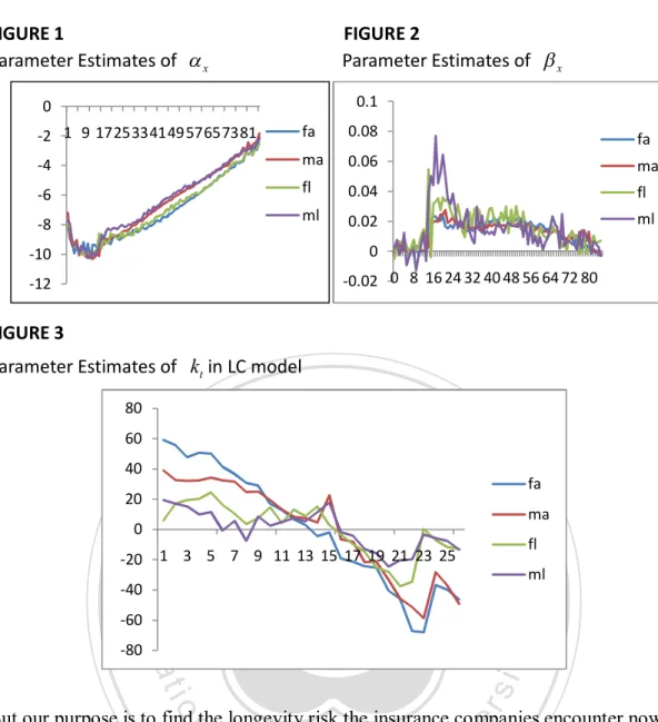
(17) Vcohort ( mxs , g , r , t ) : the product value pricing under cohort-mortality basis. We call the total difference of portfolio as difference effect of our objective function. If the insurance company put more emphasis on the variance effect, that means they tend to control the portfolios change due to the unexpected future changes in mortality rate and interest rate. If they put more emphasis on the difference effect, they lean to minimize the mispricing difference. The purpose of our paper is to find a possible products collocation in an insurance company to minimize the variance effect with a weight (1-θ) and the difference effect with a weight θ. We can adjust the significance. 政治大. of the difference effect by the weight θ. Our objective function can be expressed as. 立. 學. ‧ 國. follows:. (1   ) Var (dV )    D 2 f ( N )  min s ,g N x , NB. (23). ‧. n. al. er. io. sit. y. Nat 3. Data 3.1 Mortality Rate Data. Ch. engchi. i n U. v. The mortality data were collected via Taiwan Insurance Institute (TII) and cover all life insurance companies in Taiwan. The original data are categorized by ages, gender and sorts. We use the original data to construct four Lee-Carter mortality tables, comprising female annuity (fa), male annuity (ma), female life insurance (fl) and male life insurance (ml). The maximal age of the original data is about 85 and the estimated parameters in LC model by approximation method are as follows in Figure1-3.. 11.

(18) FIGURE 1 Parameter Estimates of  x. FIGURE 2 Parameter Estimates of  x 0.1. 0 -2 1 9 172533414957657381. fa. 0.08. fa. -4. ma. 0.06. ma. -6. fl. 0.04. fl. ml. 0.02. ml. -8. 0. -10. -0.02 0 8 16 24 32 40 48 56 64 72 80. -12. FIGURE 3 Parameter Estimates of kt in LC model 80 60. 立. 40. 政治大 fa. ‧ 國. 學. 20. 0. -20. 1 3 5 7 9 11 13 15 17 19 21 23 25. ma fl. ‧. ml. -40 -60. Nat. er. io. sit. y. -80. But our purpose is to find the longevity risk the insurance companies encounter now,. al. n. v i n C h risk if the maximal so we can not show the actual longevity age is only 85. We can engchi U. utilize extrapolation to predict the mortality rate of higher ages and set our maximal age 100. And we use the predicted mortality rate to price insurance products. In addition to the forecast of future mortality rate, we want to calculate the standard deviation (  k ) of each kt . (fa, ma, fl, and ml). TABLE 1 Standard deviation of kt in four different products. Std..  t fa.  tma. tfl.  tml. 9.34057. 10.75928. 9.89995. 8.26466. 12.

(19) Then, we use Cholesky decomposition method to transform the four original dependent random terms into the linear combination of four independent random terms. The result is shown as follows: First, we compute the correlation matrix (M) of these four time series data of kt . The resulting correlation matrix is expressed as follows,. 1 0.774017 -0.09217 0.243753     0.774017 1 -0.1304 0.358255   M  -0.09217 -0.1304 1 0.455803    1  0.243753 0.358255 0.455803 . 立. 政治大. (24). ‧ 國. 學. We use the Cholesky decomposition to find the lower triangular matrix (R), which must satisfy the condition M  R  RT and can be shown as follows:. n. al. (25). er. io. sit. y. ‧. Nat. 0 0 0   1   0.7740 0.6332 0 0   R  0.0922 0.0933 0.9914 0     0.2438 0.2678 0.5076 0.7818 . Ch. engchi. i n U. v. Therefore, we obtain the decomposed relationship of these four random terms.  dZ kA,2   1 0 0 0   dZ k 1   A,1   0 0   dZ k 2   dZ k    0.7740 0.6332   dZ kL ,2   0.0922 0.0933 0.9914 0   dZ k 3   L ,1       dZ k   0.2438 0.2678 0.5076 0.7818  dZ k 4 . (26). We find out the decomposed matrix has some negative coefficients in tfl . This result will lead to an interesting conclusion of our paper. 13.

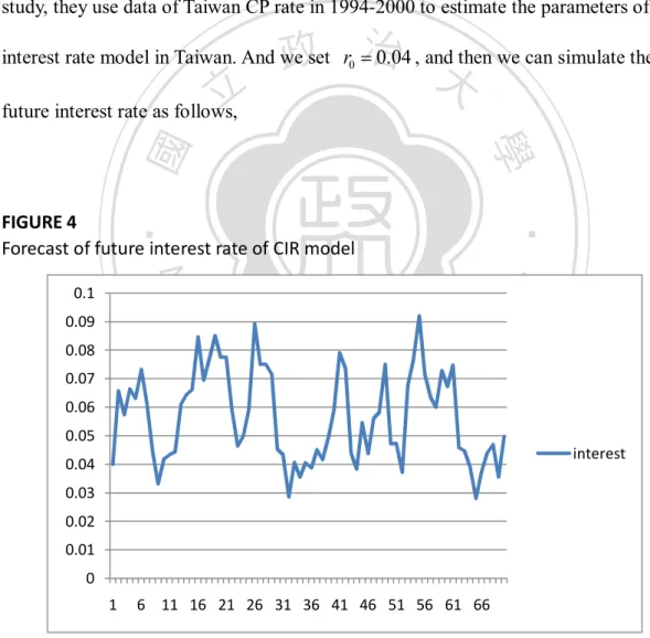
(20) 3.2 Interest Rate Data About Interest rate, we would use the ROI (return on investment) of the insurance company instead of risk-free rate in Taiwan. Because the insurance products are issued by those companies with many risks, it is not rational to use risk-free rate in our model. However, the ROI data of the insurance companies is not sufficient enough for us to find the parameters of CIR model. We use the parameters used in Chen (2002) and Lin(2004), which is (a, b,  r )  (0.16633, 0.06061, 0.04733) . In their study, they use data of Taiwan CP rate in 1994-2000 to estimate the parameters of CIR. 政治大. interest rate model in Taiwan. And we set r0  0.04 , and then we can simulate the. 立. future interest rate as follows,. ‧ 國. 學 ‧. FIGURE 4 Forecast of future interest rate of CIR model. sit. al. n. 0.08. er. io. 0.09. y. Nat. 0.1. 0.07 0.06 0.05. Ch. engchi. i n U. v. interest. 0.04 0.03 0.02 0.01 0 1. 6 11 16 21 26 31 36 41 46 51 56 61 66. 14.

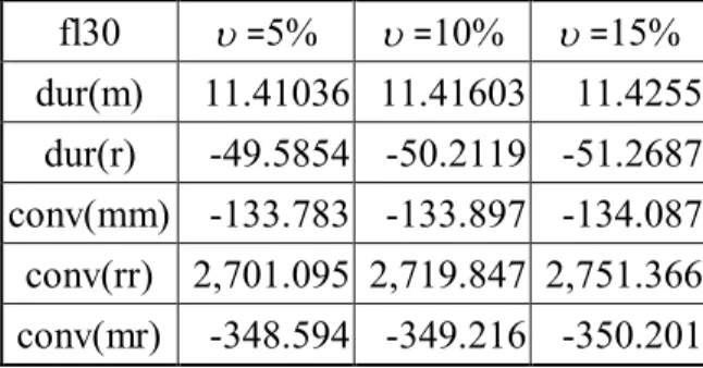
(21) 4. Numerical Analysis 4.1 Scenario 1 : θ = 0 (no period-cohort difference effect) We begin with the simple case, in which we consider the situation of only two product, annuity and life insurance. We can capture the corresponding hedging relation from those simple cases. Given one unit value of annuity due, we can find the optimal value(x) of life insurance. At first we assume the weight θ is zero, and then we can observe the effect caused by the variance term only.. 政治大 Different unexpected change rate: We assume  (the unexpected change rate of 立. future mortality rate and interest rate) can be 5%, 10%, and 15%, and Table 2 is the. ‧ 國. 學. optimal results in different unexpected change rate. f ( x)  Var ( dV ( x )). ‧ er. io. al.  =10%  =15%. 4.51×10. Ch. e n g c h i Uf(N)  =5%. 0.1353. f(N). 1.66×10-7. 1.56×10-7. N. 4.51×10-5. f(N). -7. 0.1353 1.56×10-7. 1.66×10. v nNi 4.51×10 fl30. n. fl30 ml30 -5 N 4.51×10 0.1353  =5% -7 1.56×10-7 f(N) 1.65×10 N. y 1 unit ma60. 1 unit fa60. -5. sit. Nat. TABLE 2-1 TABLE 2-2 Optimal units of life insurances with different  (θ = 0).  =10%  =15%. N f(N). 1.23×10. ml30 -5 -6. 4.51×10-5. 0.5411 1.07×10-6 0.5411. 1.23×10-6 1.07×10-6. N. 4.51×10-5. f(N). -6. 1.23×10. 0.5412 1.07×10-6. From the result above, we observe that the unexpected change rate of mortality and interest rate doesn’t have obvious impact on the optimal amount invested in life insurance. The reason is that the effective durations and convexities of each product are almost the same. We take female life insurance30 for example. 15.

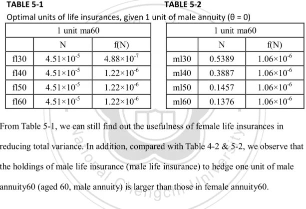
(22) TABLE 3 Effective duration (dur) and convexity (conv) with different  (5%, 10% 15%)  =5%. fl30.  =10%.  =15%. dur(m). 11.41036 11.41603. 11.4255. dur(r). -49.5854 -50.2119 -51.2687. conv(mm). -133.783 -133.897 -134.087. conv(rr). 2,701.095 2,719.847 2,751.366. conv(mr). -348.594 -349.216 -350.201. But the variance increases slightly with larger unexpected change rate because of the. 政治大. slightly larger duration and convexity. Due to this result, we use 10% unexpected. 立. change rate of mortality and interest rate to do the following scenario analyses.. ‧. ‧ 國. 學 sit. y. Nat. Given 1 unit of annuities, find the optimal units of different life insurances.. n. al. er. io. We hold fixedly 1 unit of female annuity due and try to find the corresponding. i n U. v. optimal units of different life insurances. The results are shown in tables below,. Ch. engchi. TABLE 4-1 TABLE 4-2 Optimal units of life insurances, given 1 unit of female annuity (θ = 0) 1 unit fa60 1 unit fa60 N. f(N) -5. N -7. f(N). fl30. 4.51×10. 1.66×10. ml30. 0.1226. 1.56×10-7. fl40. 4.51×10-5. 1.66×10-7. ml40. 0.0863. 1.62×10-7. fl50. 4.51×10-5. 1.66×10-7. ml50. 0.0407. 1.62×10-7. fl60. 4.51×10-5. 1.66×10-7. ml60. 0.0355. 1.62×10-7. 16.

(23) From Table 4-1, we can observe that we can not reduce the total variance by holding female life insurances, but we can make it through male life insurances from Table 4-2. The variance of ( female annuity, male life insurance) portfolios are smaller than the variance of ( female annuity, female life insurance) portfolios. Then, we hold 1 unit value of male annuity, and the following are the optimal amounts of life insurance with different genders and ages.. TABLE 5-1 TABLE 5-2 Optimal units of life insurances, given 1 unit of male annuity (θ = 0) 1 unit ma60 1 unit ma60. 立4.88×10. N -5. -7. N. f(N). ml30. 0.5389. 1.06×10-6. 學. 政治大 f(N). fl40. 4.51×10-5. 1.22×10-6. ml40. 0.3887. 1.06×10-6. fl50. 4.51×10-5. 1.22×10-6. ml50. 0.1457. 1.06×10-6. fl60. 4.51×10-5. 1.22×10-6. ml60. 0.1376. 1.06×10-6. ‧ 國. 4.51×10. ‧. fl30. sit. y. Nat. From Table 5-1, we can still find out the usefulness of female life insurances in. io. er. reducing total variance. In addition, compared with Table 4-2 & 5-2, we observe that. al. v i n C is larger than thoseUin female annuity60. annuity60 (aged 60, male annuity) h engchi n. the holdings of male life insurance (male life insurance) to hedge one unit of male. We anticipate the same result from the Cholesky decomposition and the durations of each product.  dZ kA,2   1 0 0 0   dZ k 1   A,1   0 0   dZ k 2   dZ k    0.7740 0.6332   dZ kL ,2   0.0922 0.0933 0.9914 0   dZ k 3   L ,1       dZ k   0.2438 0.2678 0.5076 0.7818  dZ k 4 . (26). In the portfolio above, all annuities will pay the payment annually after age 60. (For example, female annuity40 is a deferred-20-year annuity with the insured aged 40.) 17.

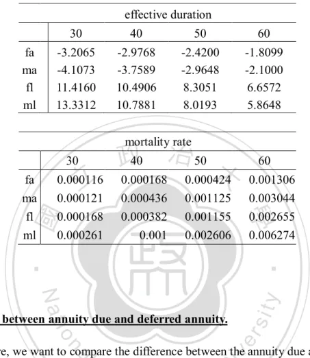
(24) The female life insurance’s variation term can be decomposed into the linear combination of three independent Brownian motions, but the coefficients of dZk1 and. dZ k 2 are negative, so we can not offset the total variance by utilizing female life insurances in order to hedge female or male annuities. Taking one unit female annuity for example, we have to minimize the variance effect of our objective function. We look into one component of the variance effect, say Q1, which is shown in formula (27). Q1 contains effective durations, mortality. 政治大 difference of beta and sigma 立in different specific product is small, so we can basically rate( mxs , g ),beta(  xs , g ),sigma(  ks , g ). In the mortality data section, we can tell that the. ‧ 國. 學. derive our finding from effective duration, mortality rate, and the coefficients in Cholesky decomposition. We will expect to hedge longevity risk of annuity product. ‧. by holding some unit of life insurance because we know the sign of effective duration. sit. y. Nat. of annuity and life insurance are opposite. But the coefficient of Cholesky. n. al. hedging effect from holding life insurance.. Ch. engchi. er. io. decomposition of female life insurance is negative, and then we can not obtain the. i n U. v.   VxA,2 A,2 A,2 A,2 VxL ,2 L ,2 L ,2 L ,2 A,2 Q1  (a11  A,2  mx   x   k )  N x  (a31  L ,2  mx   x   k )  N xL ,2  (27) mx mx   However, the coefficient of male life insurance is positive, so it is possible to minimize the variance effect by holding some male life insurance. The reason why we must hold more male life insurance to hedge male annuity60 than female annuity60 is that the magnitude of male annuity’s duration and mortality rate are larger than that of female, as shown in Table 6, so we must hold more male life insurance to hedge 1 unit of male annuity60. According to the mortality pattern of male and female, the mortality rate of males is higher than the that of female, so it is reasonable that the 18.

(25) males’ duration is larger than that of female.. TABLE 6 Effective duration and mortality rate of each product (insured) effective duration fa ma fl ml. 30. 40. 50. 60. -3.2065 -4.1073 11.4160 13.3312. -2.9768 -3.7589 10.4906 10.7881. -2.4200 -2.9648 8.3051 8.0193. -1.8099 -2.1000 6.6572 5.8648. mortality rate. 30. 立. 0.000436 0.000382 0.001. 0.001125 0.001155 0.002606. 0.001306 0.003044 0.002655 0.006274. ‧. ‧ 國. 0.000116 0.000121 0.000168 0.000261. 60. 學. fa ma fl ml. 政40 治 50 大 0.000168 0.000424. sit. y. Nat. io. n. al. er. Difference between annuity due and deferred annuity.. i n U. v. Furthermore, we want to compare the difference between the annuity due and deferred. Ch. engchi. annuity. The comparison is as follows,. TABLE 7-1 female annuity due TABLE 7-2 female deferred annuity Comparison of deferred effect of female annuity (θ = 0) 1 unit fa60 N. f(N). 1 unit fa30 N. f(N). ml30. 0.1226. 1.56×10-7. ml30. 0.0140. 2.04×10-9. ml40. 0.0863. 1.62×10-7. ml40. 0.0097. 2.04×10-9. ml50. 0.0407. 1.62×10-7. ml50. 0.0046. 2.04×10-9. ml60. 0.0355. 1.62×10-7. ml60. 0.0040. 2.04×10-9. 19.

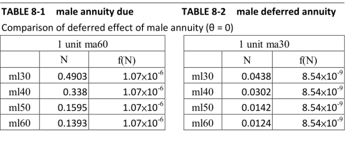
(26) TABLE 8-1 male annuity due TABLE 8-2 male deferred annuity Comparison of deferred effect of male annuity (θ = 0). ml30 ml40 ml50 ml60. 1 unit ma60 N f(N) 0.4903 1.07×10-6 0.338 1.07×10-6 0.1595 1.07×10-6 0.1393 1.07×10-6. ml30 ml40 ml50 ml60. 1 unit ma30 N f(N) 0.0438 8.54×10-9 0.0302 8.54×10-9 0.0142 8.54×10-9 0.0124 8.54×10-9. From Table 7-1 & 7-2 and Table 8-1 & 8-2, the deferred annuities need less amount of life insurances to hedge the mortality uncertainty. Although the duration of deferred. 政治大 discount effect. In addition,立 we can observe that with the ages of annuitant increase,. annuities are higher, the mortality effects of deferred annuities might be diluted by the. ‧ 國. 學. we need less and less life insurance units to hedge the corresponding annuity. Although the duration of younger-age life insurances is larger than the old-age’s, the. ‧. mortality rate of the elder is much higher than the younger’s mortality rate. Therefore,. sit. y. Nat. it is more possible for the insurance company to face an instant claim from the elder. n. al. er. io. insured. So the insurance company needs less units of the elder life insurance to offset the longevity risk of annuities.. Ch. engchi. i n U. v. Given 1 unit of life insurance, find the optimal units of different annuities. Now we hold fixedly 1 unit of life insurance and try to find the corresponding optimal units of different annuity products. Based on the outcomes above, we know that we couldn’t reduce the total variance of the changes of portfolio value by female life insurance, so we discuss the case of male life insurance only.. 20.

(27) TABLE 9-1 TABLE 9-2 Optimal units of annuity, given 1 unit of male life insurance (θ = 0) 1 unit ml30 fa30 fa40 fa50 fa60. N 4.2338 2.1993 1.0058 0.4849. 1 unit ml30 f(N) 6.16×10-7 6.16×10-7 6.16×10-7 6.16×10-7. ma30 ma40 ma50 ma60. N 2.9301 0.9929 0.4651 0.2618. f(N) 5.71×10-7 5.71×10-7 5.71×10-7 5.71×10-7. TABLE 10-1 TABLE 10-2 Optimal units of annuity, given 1 unit of male life insurance (θ = 0) 1 unit ml60 f(N) 7.64×10-6 7.64×10-6 7.64×10-6 7.64×10-6. ma50 ma60. 1.6376 0.9217. f(N) 7.08×10-6 7.08×10-6 7.08×10-6 7.08×10-6. ‧. ‧ 國. 立. N 治政 ma30 大10.317 ma40 3.4961. 學. fa30 fa40 fa50 fa60. N 14.9075 7.7440 3.5416 1.7074. 1 unit ml60. y. Nat. According to Table 9 & 10, we can hold less male annuity than female annuity to. er. io. sit. obtain our goal of hedging the given life insurance. The reason is similar to the above as the duration of male annuities are larger so we can use less male annuities to hedge. al. n. v i n male life insurance products. The we must allocate more units on deferred Creason h e nwhy gchi U annuity to hedge life insurance is the dilution of discount effect. Compared with Table 9 & 10, it is more possible for the insured of age 60 to have claim in the near future. Thus, the hedging holding of annuity is higher for the elder life insurance insured.. 4.2 Scenario 2: θ=1 (no variance effect of the change of total portfolio’s value) Without the consideration to the variance effect in our objective function, we can fixedly hold 1 unit of annuity product and find a perfect-hedge unit of life insurance product, and vice versa. So the value of objective function is always zero in the 21.

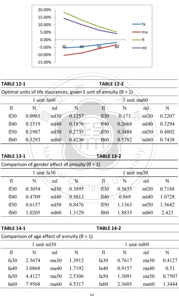
(28) optimal situation. In the following results, we just show the optimal unit of life insurance product, corresponding to fixedly holding one unit of annuity product. In Table 11 and Figure 5, we show the difference per value between period and cohort bases. We can find out that regarding to annuity products, the that of male difference is larger; however, the that of female difference is larger regarding to life insurance. Besides, we observe that the magnitude of difference between period and cohort bases decreases as the issue age increases. For a whole life insurance, the younger the issue age is, the more coverage year insurance company must cover. So the period-cohort. 政治大 younger issue-age annuities have dilution of interest rate effect ( deferred effect), but 立 pricing difference is larger with younger issue age. As to annuity, although the. due to the every-year improvement of mortality rate, the difference between period. ‧ 國. 學. and cohort mortality rate become larger and larger as time goes by. So the. ‧. improvement of mortality rate of younger-issue-age annuity is larger than the. sit. y. Nat. improvement of elder-issue-age annuity. According to Table 12-14, comparing the. io. er. results in Scenario 2 with the results in Scenario 1, we can hedge longevity risk of annuity products through female life insurance products in Scenario 2. However, with. al. n. v i n C htendency goes up.UThis outcome is totally different the issue age increases, the holding engchi from the results in Scenario 1.. TABLE 11 The pricing differences of each product between period and cohort bases Vperiod-Vcohort fa ma fl ml. 30. 40. 50. 60. -5.43% -10.44% 18.28% 14.32%. -4.73% -8.81% 13.17% 10.10%. -3.30% -5.90% 8.60% 6.39%. -1.83% -3.25% 5.16% 4.01%. 22.

(29) FIGURE 5 The pricing differences of each product between period and cohort bases 20.00% 15.00% 10.00%. fa. 5.00%. ma. 0.00%. fl 30. -5.00%. 40. 50. 60. ml. -10.00% -15.00%. TABLE 12-2 治政1 unit of annuity大(θ = 1) Optimal units of life insurances, given 1 unit fa60 1 unit ma60 立 fl N ml N fl N ml ml30 ml40 ml50 ml60. 0.1257 0.1876 0.2735 0.4236. fl30 fl40 fl50 fl60. n. er. io. al. fl fl30 fl40 fl50 fl60. N 0.3054 0.4709 0.6157 1.0205. ml ml30 ml40 ml50 ml60. sit. TABLE 13-2. Comparison of gender effect of annuity (θ = 1) 1 unit fa30. ml30 ml40 ml50 ml60. N 0.2207 0.3294 0.4802 0.7438. y. Nat. TABLE 13-1. 0.173 0.2668 0.3488 0.5782. ‧. 0.0985 0.1519 0.1987 0.3293. 學. fl30 fl40 fl50 fl60. ‧ 國. TABLE 12-1. i n N U. v. 1 unit ma30. C hN. fl e hi n 0.3895 g cfl30 0.5813 0.8476 1.3129. fl40 fl50 fl60. TABLE 14-1. 0.5635 0.869 1.1363 1.8833. ml ml30 ml40 ml50 ml60. N 0.7188 1.0728 1.5642 2.423. TABLE 14-2. Comparison of age effect of annuity (θ = 1) 1 unit ml30 fl fa30 fa40 fa50 fa60. N 2.5674 3.0868 4.4127 7.9568. ml ma30 ma40 ma50 ma60. 1 unit ml60 N 1.3912 1.7192 2.5306 4.5317. fl fa30 fa40 fa50 fa60 23. N 0.7617 0.9157 1.3091 2.3605. ml ma30 ma40 ma50 ma60. N 0.4127 0.51 0.7507 1.3444.

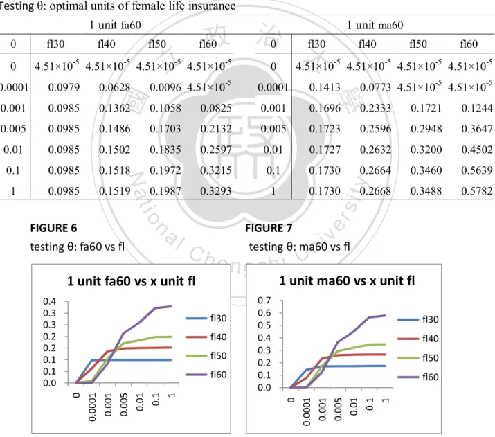
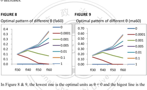
(30) 4.3 Scenario 3: 0 < θ <1 ( both of variance effect and period-cohort effect) Testing the weight θ Now we want to discuss how much weight to put on the difference effect. We consider holding 1 unit of annuity due and try to find the optimal units of life insurance. At first, we use different female life insurances to obtain hedging effect. The results are expressed in Table 15 and Figure 6 & 7. TABLE 15-1. TABLE 15-2. Testing θ: optimal units of female life insurance. 政治θ 大 fl60 fl30. 1 unit fa60 θ 0. fl30. fl40. fl50. 立. 4.51×10-5 4.51×10-5 4.51×10-5 4.51×10-5. 1 unit ma60 fl40. fl50. fl60. 4.51×10-5 4.51×10-5 4.51×10-5 4.51×10-5. 0. 0.0628. 0.0096 4.51×10-5. 0.0001. 0.1413. 0.0773 4.51×10-5 4.51×10-5. 0.001. 0.0985. 0.1362. 0.1058. 0.0825. 0.001. 0.1696. 0.2333. 0.1721. 0.1244. 0.005. 0.0985. 0.1486. 0.1703. 0.2132. 0.005. 0.1723. 0.2596. 0.2948. 0.3647. 0.01. 0.0985. 0.1502. 0.1835. 0.2597. 0.01. 0.1727. 0.2632. 0.3200. 0.4502. 0.1. 0.0985. 0.1518. 0.1972. 0.3215. 0.1. 0.1730. 0.2664. 0.3460. 0.5639. 1. 0.0985. 0.1519. 0.1987. 0.3293. 1. 0.1730. 0.3488. 0.5782. n. Ch. fl40 fl50. 1. 0.1. fl60 0. 1. 0.1. 0.01. 0.005. fl60. fl30. 0.01. fl50. 0.001. y. 0.7 0.6 0.5 0.4 0.3 0.2 0.1 0.0. fl40. 0.0001. sit. 1 unit ma60 vs x unit fl. fl30. 0. v. 0.005. 0.4 0.3 0.3 0.2 0.2 0.1 0.1 0.0. engchi. i n U. 0.001. 1 unit fa60 vs x unit fl. FIGURE 7 testing θ: ma60 vs fl. 0.0001. io. al. 0.2668. er. Nat. FIGURE 6 testing θ: fa60 vs fl. ‧. ‧ 國. 0.0979. 學. 0.0001. From Table 15 and Fig 6 & 7, we observe that the optimal unit of female life insurance decreases as the weight θ decreases. That is, when we put less emphasis on 24.

(31) difference effect, we tend to minimize the variation of the change of total portfolio’s value, so the less unit of life insurance we hold, the smaller the objective function is. According to Fig 8 &9, the patterns of female annuity60 and ma60 are similar, but the magnitude of ma60 is larger than female annuity60, which is the same result as in Scenario 1 & 2 mentioned above. In addition, we find the female life insurances are unable to reduce the variance of total portfolio’s value in Scenario 1, and that is the reason why we need less and less unit or even zero unit of life insurance as the weight θ decreases.. 治9 政 FIGURE 大 Optimal pattern of different θ (fa60) Optimal pattern of different θ (ma60) 立 0 0.70 0 FIGURE 8. fl50. 0.1 1 fl60. io. fl30. n. al. 0.001 0.005 0.01 0.1. y. 0.01. fl40. sit. 0.005. 0.0001. fl50. 1 fl60. er. fl40. 0.001. Nat. fl30. 0.60 0.50 0.40 0.30 0.20 0.10 0.00. ‧. ‧ 國. 0.0001. 學. 0.4 0.3 0.3 0.2 0.2 0.1 0.1 0.0. Ch. i n U. v. In Figure 8 & 9, the lowest one is the optimal units as θ = 0 and the higest line is the. engchi. optimal units as θ =1. As θ = 0.1, 0.001, and 0.005 respectively, the pattern is similar to the case with θ =1. In the case of θ = 0.001, we find out the pattern is similar to the case of θ =1 in younger age, but in older ages the pattern will decrease like the case of θ = 0. In Scenario 1, we observe that the variance effect is stronger in older age because the variance effect is positively related to the mortality rate and effective duration. So we can observe the interaction of both variance and difference effect in the case of θ = 0.001. In Table 16, we investigate the collocation of annuity due and different male life insurances, and the results are shown as follows, 25.

(32) TABLE 16-1. TABLE 16-2. Testing θ: optimal units of male life insurance 1 unit fa60 ml30. 0. ml40. ml50. ml60. θ. ml30. 0.1226 0.0863 0.0407. 0.0355. 0. 0.4903. 0.338. 0.1595. 0.1393. 0.0001 0.1249 0.1269 0.0560. 0.0440. 0.0001. 0.2857. 0.3345. 0.1805. 0.1525. 0.001. 0.1256 0.1744 0.1368. 0.1064. 0.001. 0.229. 0.3305. 0.2919. 0.2497. 0.005. 0.1257 0.1847 0.2221. 0.2407. 0.005. 0.2224. 0.3296. 0.4094. 0.4589. 0.01. 0.1257 0.1861 0.2447. 0.3044. 0.01. 0.2215. 0.3295. 0.4406. 0.5581. 0.1. 0.1257 0.1874 0.2706. 0.4086. 0.1. 0.2207. 0.3294. 0.4762. 0.7204. 1. 0.1257 0.1876 0.2735. 0.4236. 1. 0.2207. 0.3294. 0.4802. 0.7438. 政治大. 立. ‧ 國. ml50. 0.4. y. ml60. sit. ml50. 0.2 0. 1. 0.1. Ch. ml40 ml60. v. 0 0.0001 0.001 0.005 0.01 0.1 1. 0.01. 0.005. ml30. n. 0.001. io. 0.0001. ‧. 0.8 0.6. ml40. Nat 0. 1 unit ma60 vs x unit ml ml30. al. ml60. FIGURE 11 testing θ: ma60 vs ml. 1 unit fa60 vs x unit ml 0.5 0.4 0.3 0.2 0.1 0. ml50. 學. FIGURE 10 testing θ: fa60 vs ml. ml40. er. θ. 1 unit ma60. engchi. i n U. Compared the result in Table 16 with the result in Table 15, the optimal unit of male life insurance is not always decreasing as the weight θ decreases. In Scenario 1, we can utilize male life insurances to reduce total variance term, but we also take period-cohort difference into consideration at the same time. So the outcomes in Table 15 & 16 are the interaction between these two effects.. 26.

(33) FIGURE 12 Optimal pattern of different θ (fa60). FIGURE 13 Optimal pattern of different θ (ma60). 0.5. 0. 0.8. 0.4. 0.0001. 0.6. 0.3. 0.001. 0.2. 0.005. 0.005 0.01 0.1. 0. 1. ml30 ml40 ml50 ml60. 0.001. 0.2. 0.1. 0. 0.0001. 0.4. 0.01. 0.1. 0. ml30 ml40 ml50 ml60. 1. From the observation above, we choose the weight θ=0.001 because there exists. 政治大. obvious interaction between two effects. The results with weight θ=0.001 are. 立. expressed as follows,. ‧. ‧ 國. 學. 0.0985. fl40. 0.1362. fl50. 0.1058. fl60. 0.0825. f(N). N. 1.66×10-7. ml30. 0.1256. a l 2.05×10 v i ml40 0.1744 n Ch 3.28×10 e n g cml50 h i U 0.1368. n. fl30. io. N. 1 unit fa60. sit. 1 unit fa60. er. Nat. y. TABLE 17-1 TABLE 17-2 Optimal units of life insurance, given 1 unit of female annuity (θ = 0.001) f(N) 1.56×10-7. -7. 1.74×10-7. -7. 3.01×10-7. 4.18×10-7. ml60. 0.1064. 3.85×10-7. TABLE 18-1 TABLE 18-2 Optimal units of life insurance, given 1 unit of male annuity (θ = 0.001) 1 unit ma60 N. 1 unit ma60 f(N). N. f(N). fl30. 0.1696. 1.26×10-6. ml30. 0.229. 1.11×10-6. fl40. 0.2333. 1.39×10-6. ml40. 0.3305. 1.07×10-6. fl50. 0.1721. 1.80×10-6. ml50. 0.2919. 1.33×10-6. fl60. 0.1244. 2.06×10-6. ml60. 0.2497. 1.61×10-6. 27.

(34) TABLE 19-1 TABLE 19-2 Comparison of age effect of female annuity (θ = 0.001) 1 unit fa60. 1 unit fa30. x. f(x). x. f(x). -7. ml30. 0.3779. 9.15×10-8. ml30. 0.1256. 1.56×10. ml40. 0.1744. 1.74×10-7. ml40. 0.5072. 3.94×10-7. ml50. 0.1368. 3.01×10-7. ml50. 0.3527. 1.82×10-6. ml60. 0.1064. 3.85×10-7. ml60. 0.2431. 2.54×10-6. TABLE 20-1 θ=0.001, ma60 vs. ml TABLE 20-2 θ=0.001, ma30 vs. ml Comparison of age effect of male annuity (θ = 1) 1 unit ma60. 1 unit ma30. N 治政 1.11×10 ml30 大 0.698 ml40 0.9377 立1.07×10. N. f(N). f(N). -6. 2.98×10-7. -6. 1.31×10-6. ml40. 0.3305. ml50. 0.2919. 1.33×10-6. ml50. 0.6543. 6.15×10-6. ml60. 0.2497. 1.61×10-6. ml60. 0.4528. 8.62×10-6. ‧. ‧ 國. 0.229. 學. ml30. sit. io. optimal unit of fl with respect to one unit of different annuity. n. er. optimal unit of fl with respect to one unit of different annuity. al. 0.9 0.8 0.7 0.6 0.5 0.4 0.3 0.2 0.1 0. y. Nat. FIGURE 14 FIGURE 15 optimal units of fl (ml), given 1 unit of different annuities. Ch. 1 e hi n c g fa60. i n U. v. 0.8. ma60. fl40. fl50. fa30. 0.4. ma30. fl30. ma60. 0.6. fa30. fa60. ma30. 0.2 0. fl60. ml30 ml40 ml50 ml60. From Figure 14 and 15, we find out the patterns are similar in different annuities. The biggest difference is the magnitude of optimal unit.. 28.

(35) 4.4 General Portfolio of Insurance Products Based on the results above, we can expand our products to a general portfolio for an insurance company, that is, there are many life insurances and annuities with different ages and genders. In our study, we consider a general portfolio comprising 16 products, female annuity, male annuity, female life insurance, and male life insurance with 4 different ages (30, 40, 50, and 60). In addition, we add a zero coupon bond N(B) to hedge interest rate. The following is the historic data of the allocated amounts in different insurance. 政治大. product in 2007.. 立historic allocated amounts in 2007 40. 50. 33,394 26,866 13,109 17,081. 37,845 23,500 14,752 17,676. 62,629 31,366 20,036 20,265. 60. 43,224 21,898 7,819 8,441. Nat. sit. y. ‧. fa ma fl ml. 30. 學. ‧ 國. TABLE 21. io. er. We can calculate the value of our objective function in this historic data and find out f(N)= 3.36×104, N(B)= -704,100. It is the benchmark of our following possible. n. al. strategy.. Ch. engchi. i n U. v. We want to find a possible strategy for insurance companies to naturally hedge the longevity risk. In this section, we assume the units of life insurances are given from the historic data and try to find a optimal allocation of annuities for insurance companies. There are two methods of our proposed possible strategy. The first one is that we can make a small proportional adjustment based on the historic data. As in Table 22, N(1)=33394, and so on.. 29.

(36) TABLE 22. small proportional adjustment of historic data 30. 40. 50. 60. fa. (1±ρ%)N(1). (1±ρ%)N(2). (1±ρ%)N(3). (1±ρ%)N(4). ma. (1±ρ%)N(5). (1±ρ%)N(6). (1±ρ%)N(7). (1±ρ%)N(8). fl ml. 13,109 17,081. 14,752 17,676. 20,036 20,265. 7,819 8,441. N(1) is the historic units of fa30, that is, 33,394, and so on. ρ is the adjustment proportional level we allow to make in a insurance company. (1) ρ=10: If we allow the insurance company to adjust within 10% proportion, the result would be as follows,. 學. 30,050. N(6). 21,150. N(2). 34,060. N(7). 28,230. N(3). 56,370. N(8). 19,710. N(4). 40,330. N(B). -635,120. 24,180. f(N). 3.07×104. y. er. io. sit. N(5). ‧. N(1). Nat. ‧ 國. 立. 政治大. al. n. v i n (2) ρ=15: If we allow the insurance C hcompany to adjustUwithin 15% proportion, the engchi result would be as follows,. N(1). 28,380. N(6). 19,980. N(2). 32,170. N(7). 26,660. N(3). 57,220. N(8). 19,310. N(4). 40,750. N(B). -611,390. N(5). 22,840. f(N). 3.03×104. 30.

(37) (3) ρ=20: If we allow the insurance company to adjust within 20% proportion, the result would be as follows, N(1). 27,470. N(6). 19,300. N(2). 33,060. N(7). 28,290. N(3). 59,380. N(8). 20,330. N(4). 41,730. N(B). -612,330. N(5). 21,490. f(N). 3.00×104. When the adjustment level is 10%, we can optimize our objective function by 3.07×104. However, when the adjustment level is 15% and 20% , we can optimize our. 政治大. objective function by 3.03×104 and 3.00×104 respectively.. 立. From (1)~(3), we observe that we can minimize our objective function if we loosen. ‧ 國. 學. the allowable level of adjustment. We take the case ρ= 15 for example and show the. ‧. figure as following. In Figure 16 & 17, op(fa) is the optimal units of natural hedging strategy; the upper bound is (1+15%) multiple of historic amounts and the lower. y. Nat. n. er. io. al. sit. bound is (1-15%) multiple of historic amounts.. i n U. v. FIGURE 16 FIGURE 17 Optimal collocation under the allowable 15% adjustment level. Ch. engchi 40000 35000 30000 25000 20000 15000 10000 5000 0. fa. 80000 70000 60000 50000 40000 30000 20000 10000 0. op(fa) upper bound lower bound. 30. 40. 50. 60. ma op(ma) upper bound lower bound. 30. 40. 50. 60. The second one is that we assume the proportions of annuities are fixed based on the historic data. Then we can use the allocated value of female annuity30 and male 31.

(38) annuity30 in 2007 as a basis, so the possible optimal collocation is shown below,. TABLE 23. the proportions of annuities are fixed 30. 40. 50. 60. fa. 1.000*N(1) 1.133*N(1). 1.875*N(1). 1.294*N(1). ma fl ml. 1.000*N(2) 0.875*N(2) 13,109 14,752 17,081 17,676. 1.168*N(2) 20,036 20,265. 0.815*N(2) 7,819 8,441. 政治大. In female annuity (or male annuity), we use the unit of age 30 to be the basis and. 立. fixed the proportion. We can find the optimal value of N(1), N(2) and N(B) is 26,530. ‧ 國. 學. and 22,070 and -566,740 respectively and the value of objective function is 3.14×104. So the optimal units of these annuities are shown in the Figure 18 below:. al. n. 60000 50000 40000. y. sit. er. io. 70000. ‧. Nat. FIGURE 18 Optimal pattern in the case of fixed proportions of annuities. Ch. 30000. engchi. i n U. vfa. ma op(fa). 20000 op(ma). 10000 0 30. 40. 50. 32. 60.

(39) 5. Conclusion and Suggestion In this paper, we propose a natural hedging model, which can take care of two important effects of mortality risk at the same time. The first one is the variance of the change of total portfolio’s value, and the second is the period-cohort difference. We can hedge variations of the future mortality rate by the first effect, and hedge the present mispricing by the second one. The precedent research on natural hedging only takes care of only one of the two effects, but we incorporate these two effects into our model in this paper. Another. 政治大 insurance companies rather立 than population mortality rates. We can distinguish. difference from previous literatures, we use the experienced mortality rates from life. ‧ 國. 學. different mortality rates from this precious data. The last difference from precedent research is that our model is a general portfolio for insurance companies, so it is easier. ‧. to apply this model into practice.. y. Nat. sit. On the basis of the experienced mortality rates, we separate the mortality rate from. n. al. er. io. gender and the type of insurance products, life insurance and annuity. We can use the. i n U. v. correlation between these four types of mortality rates to hedge variations of the. Ch. engchi. future mortality rate. Furthermore, we use Lee-Carter model to forecast the future mortality rate and calculate the pricing mistake in present. Then, we can decide the relative significance of the first and second effects by a weight θ. So we can effectively apply the natural hedging strategy to a more general portfolio for life insurance companies. In the beginning of our paper, we discuss some simple cases (one annuity to one life insurance) and use these simple cases to clearly demonstrate the trend and inclination of the allocation between products in order to achieve the natural hedging. 33.

(40) objective. The last section of our paper, we discuss the general case and propose some useful and possible allocation strategies for insurance companies to hedge the mortality risk. In our study, we have two effects in our objective function. When we consider the variance effect only, the optimal units of life insurance is affected by the effective duration and mortality rate mostly. So the optimal unit of life insurance decreases as the age of life insurer increases. However, when we consider the difference effect only, the optimal unit is totally decided by the period-cohort difference of each product. So. 政治大 sensitivity of θ and find out立 there is interaction between variance and difference effect we can come to an opposite conclusion in the variance effect case. Then, we test the. ‧ 國. 學. as we set θ one. We observe that the pattern of optimal life insurance unit is similar to the difference effect in younger age, but in older age the pattern will decrease as in the. ‧. variance effect case. The reason is that the variance effect is positively related to the. sit. y. Nat. effective duration and mortality rate, so the pattern in older age will decrease as the. n. al. er. io. case of θ=0. In the general portfolio case, we use the historic allocated value in 2007. v. as a benchmark to compare the following possible strategies. As a result, we can. Ch. engchi. i n U. reduce the value of objective function by our strategies and those strategies are easier to implement in practice. However, there are still rooms for improvement in our paper. Lee-Carter model is a popular and easily-implemented mortality model since this model has been proposed, but it is merely an one-factor model. In the future, we can try to construct our model on more complicated mortality model, CBD model for example. Regarding to the interest rate, it is hard to collect sufficient ROI information of insurance company, so we just use the Taiwan CP rate to estimate the parameters in CIR model. However, is it fair to price insurance products with CP rate rather than ROI of insurance company? 34.

(41) Another suggestion is that the later literature can incorporate the hedging cost into the model, so we can compare the advantages and disadvantages of natural hedging and other hedging methods, such as buying mortality derivatives. That will lead to a more general model for natural hedging.. 6. References Carter, L. R. and Lee, R. D. (1992) “Modeling and forecasting U.S. mortality”, Journal of the American Statistical Association, 87(419): 659-675. 立. 政治大. W. Lo(1995) “The Research of Pricing in Taiwan Bills Market”. ‧ 國. 學. D. Blake and W. Burrows (2001). “Survivor bonds: helping to hedge mortality risk”, Journal of Risk and Insurance 68: 339-348. ‧. S.C. Chen (2002) “The Evaluation of Value at Risk on Taiwan Bills Portfolio”. n. al. er. io. sit. y. Nat. N. Brouhns, M. Denuit and J.K. Vermunt (2002) “A Poisson log-bilinear regression approach to the construction of projected life-tables”, Mathematics and Economics, 31: 373-393. i n U. v. J. L. Wang, L. Y. Yang, and Y. C. Pan (2003). “Hedging Longevity Risk in Life Insurance Companies”, In Asia-Pacific Risk and Insurance Association, 2003 Annual Meeting. Ch. engchi. Renshaw, A. E. and Haberman, S. (2003) “ Lee-Carter mortality forecasting with age specific enhancement”, Mathematics and Economics, 33: 255-272 Y. Lin, and S. H. Cox (2004). “Natural hedging of life and annuity mortality risks”, Mimeo. Georgia State University Y. Lin, and S. H. Cox (2005) “Securitization of Mortality Risks in Life Annuities”, Journal of Risk & Insurance, 72: 227-252 MC Koissi, AF Shapiro, G Högnäs (2006) “Evaluating and extending the Lee–Carter model for mortality forecasting: Bootstrap confidence interval”, Mathematics and Economics, 38: 1-20. 35.

(42) A. Melnikov and Y. Romaniuk (2006) “Evaluating the performance of Gompertz, Makeham and Lee–Carter mortality models for risk management with unit-linked contracts”, Mathematics and Economics, 39: 310-329 K. Dowd, D. Blake, A. J. G. Cairns and P. Dawson (2006) “Survivor Swaps”, Journal of Risk & Insurance, 73: 1-17 Cairns, A.J.G., Blake, D., and Dowd, K. (2006b) “A Two-Factor Model for Stochastic Mortality with Parameter Uncertainty: Theory and Calibration”, Journal of Risk and Insurance, 73: 687-718 J. L. Wang, H.C. Huang, S. S. Yang, J. T. Tsai (2010) “An Optimal Product Mix For Hedging Longevity Risk in Life Insurance Companies: The Immunization Theory Approach”, Journal of Risk and Insurance, 77: 473-497. 立. 政治大. ‧. ‧ 國. 學. n. er. io. sit. y. Nat. al. Ch. engchi. 36. i n U. v.

(43)