國 立 交 通 大 學
應用數學系
碩 士 論 文
分散式排程下的解決極小控制集問題的
高效率自我穩定演算法
An efficient self-stabilizing algorithm for the minimal
dominating set problem under a distributed
scheduler
研 究 生:蔡詩妤
指導教授:陳秋媛 教授
中 華 民 國 一百 年 六 月
分散式排程下的解決極小控制集問題的
高效率自我穩定演算法
An efficient self-stabilizing algorithm for the minimal
dominating set problem under a distributed scheduler
研 究 生:蔡詩妤 Student:Shih-Yu Tsai
指導教授:陳秋媛 Advisor:Chiu-Yuan Chen
國 立 交 通 大 學
應 用 數 學 系
碩 士 論 文
A Thesis
Submitted to Department of Applied Mathematics
College of Science
National Chiao Tung University
in Partial Fulfillment of the Requirements
for the Degree of
Master
in
Applied Mathematics
June 2011
Hsinchu, Taiwan, Republic of China
中 華 民 國 一百 年 六 月
分散式排程下的解決極小控制集問題的
高效率自我穩定演算法
研究生:蔡詩妤
指導老師:陳秋媛 教授
國 立 交 通 大 學
應 用 數 學 系
摘 要
本篇論文考慮的是設計解決極小控制集(MDS)問題的更具有效率的自我穩定 演算法(self-stabilizing algorithms)。
設 n 為分散式系統裡的節點數目。若一個自 我穩定演算法在給定的分散式系統執行至多 t 次動作後,即可到達合理狀態 (legitimate configuration),則稱此自我穩定演算法為 t -動作演算法( t -move algorithm)。在 2007 年,Turau 提出了一個分散式排程下的解決 MDS 問題的9n -動作演算法。隨後,在 2008 年,Goddard 等人提出一個分散式排程下的解決 MDS 問題的5n-動作演算法。設計一個執行動作少於5n次的分散式排程下的解決 MDS 問題的演算法,確實是一個挑戰。本篇論文的目的就在於設計出這樣的演 算法。具體來說,我們提出了一個分散式排程下的解決 MDS 問題的4n-動作演 算法;此外,採用我們演算法,需要4n−1個動作才可以到達合理狀態的例子也 被提出。 關鍵詞:自我穩定演算法,容錯,分散式計算,圖形演算法,控制。 中 華 民 國 一 百 年 六 月An efficient self-stabilizing algorithm for the minimal
dominating set problem under a distributed scheduler
Student: Shihyu Tsai
Advisor: Chiuyuan Chen
Department of Applied Mathematics National Chiao Tung University
Abstract
This thesis considers designing efficient self-stabilizing algorithms for solving the minimal dominating set (MDS) problem. Let n denote the number of nodes in a distributed system. A self-stabilizing algorithm is said to be a t-move algorithm if when it is used, a given distributed system takes at most t moves to reach a legitimate configuration. In 2007, Turau proposed a 9n-move algorithm for the MDS problem under a distributed scheduler. Later, in 2008, Goddard et al. proposed a 5n-move algorithm for the MDS problem under a distributed scheduler. It is indeed a challenge to develop an algorithm that takes less than 5n moves under a distributed scheduler. The purpose of this thesis is to propose such an algorithm. In particular, we propose a 4n-move algorithm under a distributed scheduler; an example such that our algorithm takes 4n− 1 moves to reach a legitimate configuration has also been proposed.
Keywords: Self-stabilizing algorithms; Fault tolerance; Distributed computing; Graph algorithms; Domination.
iii
誌
謝
在碩士期間,我把所有的心力幾乎都放在這一論文上,而可以這麼順利的產出我這 人生中第一篇論文,最想感謝的莫過於是陳秋媛老師,老師在非常忙碌的狀態下,還是 願意排出時間和我探討研究的主題,仔細凝聽我的新發展或是挫折。除了學術上的幫忙, 老師也總是願意傾聽我在人生道路上的迷惘,給我一些意見,好讓我可以靜下心來思考 正在面對的問題。另外想感謝藍國元、邱鈺傑、吳思賢學長和何恭毅同學,在我正研究 或是其它有興趣的主題上給了一些不同方向的看法,這些都讓我研究的眼界變得再廣一 點。接著感謝學長姐、同學、學弟妹們忍著睡意聽我的各種 presentation,訓練我演講 的功力。再來是陳宏賓學長教了我做研究的態度,我想研究是急不來的,研究時走了錯 的方向時,並不需要氣餒,那些經驗正是別人怎也偷不走的寶藏。 接著我還想感謝校女籃的大家,教練和隊友們,相處時間雖然很短暫,但真的很謝 謝妳們包容我的一切,使我體驗到什麼才叫毅力,什麼叫做極限,什麼叫作夥伴,什麼 叫做合作。祝福大家有著豐富的生活,真的很懷念大家。另外要感謝系女籃,每次都可 以開開心心地打各種比賽,敏筠:謝謝妳總是聽我的煩惱,也謝謝妳這麼看重我的防守, 哈。不可能忘記小巴的左手上籃,裴的三分王,爆氣學姊等,對了還有謝謝默默的幫手 們(噓,秘密)。 最後想感謝研究室友們包容我的爆氣,小泡總是陪我看貓咪(謝謝阿吉先生和小鳳 梨的陪伴,啾),小太總是在研究室讓我不孤單,小 P、美女會說一些有趣的數學問題, student 的莫名表情,猴子的探討未來議題,這些都讓我的生活生色許多。 事實上已經在交通大學應用數學系唸了六年的書,體驗了很多的第一次,有欣喜、 有悲傷,這段期間,無疑是我人生的轉淚點。我必然要感謝父蔡英吉先生和母楊錦女士 的養育之恩,讓我長成這樣一個健全的身心,才能夠用積極的態度去面對生命中的挫折, 健康的身體享受這一切。接著想要感謝我的摯友、家人、兼摯愛:楊晧琮,總是在身邊 陪伴我走過這些開心、難過,謝謝。 再來是親朋好友的關懷和玩耍,還有所有出現在這時期的人事物,我都想感謝,謝 謝你們之於我的養成。祝福大家享受生命。 蔡詩妤 民國一百年六月二十七日 於新竹Contents
Abstract (in Chinese) i
Abstract (in English) ii
Acknowledgement iii Contents iv List of Figures v List of Tables v 1 Introduction 1 2 Related works 5
3 Our main result 6
3.1 Our algorithm . . . 6 3.2 Correction and convergence . . . 9
List of Figures
1 The state diagram of our algorithm. . . 8 2 An example of our algorithm. . . 18 3 An example such that our algorithm takes 4n−1 moves to reach a legitimate
configuration. . . 20
List of Tables
1 Self-stabilizing minimal dominating set algorithms. . . 5 2 The executed rules in every rounds. . . 20
1
Introduction
Self-stabilization is a fault-tolerance approach for distributed systems and was intro-duced by Dijkstra in 1974 in [1]. Intuitively, a self-stabilizing system guarantees to reach a correct configuration, in a finite time, regardless of its initial configuration. Here, the configuration of a distributed system (also called the state) consists of the state of ev-ery process. More precisely, a distributed system is self-stabilizing if it has the following two properties: convergence property and closure property. The convergence property is: starting from an illegitimate (incorrect) configuration, the distributed system must reach a legitimate (correct) configuration in a finite time. The closure property is: after reaching a legitimate configuration, the system must remain in the set of legitimate configurations. Hence a self-stabilizing system can recover from any transient fault without any external intervention.
In this thesis, we will consider a distributed system whose topology is represented by an undirected graph G = (V, E), where the nodes represent the processes and the edges represent the interconnections between the processes. Throughout this paper, we use n to denote the number of nodes in the graph G. Let v be a node. A node u is a neighbor of v if they are adjacent. We use N (v) to denote the set of neighbors of v. Note that we use the terms node and process interchangeably.
There are two common models of interprocess communication in distributed systems: the message-passing model and the shared-memory model. In the message-passing model, the processes exchange messages with one another in order to transfer information. In the shared-memory model, processes use the shared memory create and the shared memory attach system calls to create and to gain access to regions of the memory owned by other processes. Do notice that self-stabilizing algorithms usually use the shared-memory model, where neighboring processes may communicate via common variables or registers. Since
the operating system normally tries to prevent one process from accessing the memory of another process, the shared memory model requires that two or more processes agree to remove this restriction so that they can exchange information by reading and writing data in the shared areas. The processes are also responsible for ensuring that they will not write to the same location simultaneously.
The self-stabilizing program of each node consists of a collection of rules of the form: ⟨precondition⟩ −→ ⟨statement⟩.
The precondition of a rule is a Boolean expression formed by state of the node and the states of its neighboring nodes. The statement of a rule will only update the state of the node. The execution of a statement is called a move. A rule is called enabled if its precondition evaluates to be true. A node is called enabled (also called privileged) if at least one of its rules enabled. We assume that rules are atomically execute, in other words, the evaluation of a precondition and the move are performed in one atomic step. Self-stabilizing systems operate in rounds. In every round, first, all nodes check the preconditions of their rules. An enabled node makes its move means that it is brought into a new state determined by its old state and the states of its neighboring nodes. Notice that slightly different definitions for what is a round are given in the literature. In this thesis, a round is defined to be the minimum time period in which every node has been scheduled to execute a rule at least once.
In distributed systems, each node performs a sequence of atomic steps, where an atomic step is the “largest” step guaranteed to be executed uninterruptedly; see [3]. An algorithm of a distributed system is said to use composite atomicity if some atomic step contains (at least) a read operation and a write operation and to use read/write atomicity if each atomic step contains either a single read operation or a single write operation but not both.
models are encapsulated within the notion of a scheduler (also called daemon). Common schedulers are central schedulers, synchronous schedulers, and distributed schedulers. Un-der a central scheduler, only one enabled node can execute an atomic step at one time. Under a synchronous scheduler (also called fully distributed), all enabled nodes will ex-ecute an atomic step at the same time. Under a distributed scheduler, a subset of the enabled nodes execute an atomic step at the same time. The above schedulers are the most popular schedulers; variants of them have also been proposed.
In a distributed system, an execution can be viewed as a sequence of moves (i.e., atomic steps) made by nodes. At any instance in time, a number of moves at nodes are possible but usually only a subset of these are made due to lack of any synchrony. An enabled node can be disabled either by a move or by moves made by the node itself or the neighboring nodes. Notice that although it is easier to prove stabilization for algorithms working under central schedulers, synchronous and distributed schedulers are more suitable for practical implementations.
The stabilization time is the maximum amount of time it takes for the system to reach a legitimate configuration. The stabilization time is often used to serve as the time complexity of a self-stabilizing algorithm and is in terms of moves or rounds. For a synchronous scheduler, all enabled nodes make their moves in one round; however, for a distributed scheduler, only a selected subset of enabled nodes make their moves in one round. Thus when stabilization time is considered, the number of moves is in general an upper bound on the number of rounds; see Table 1.
Let G = (V, E) be a given graph (distributed system). An independent set S of G is a subset of V such that each pair of nodes in S are not adjacent. S is a maximal independent set of G if for any v ̸∈ S, the set S ∪ {v} is not an independent set of G. A dominating set S of G is a subset of V such that each v ∈ V \ S has at least one neighbor in S. S is a minimal dominating set of G if for any v ∈ S, the set S \ {v} is not a dominating
set of G. For convenience, we use MIS and MDS to denote maximal independent set and minimal dominating set, respectively. The MDS (resp., MIS) problem is the problem of finding an MDS (resp. MIS) for a given graph. Both problems have attracted a lot of research interests. In a distributed system, an MDS is maintained to optimize the number and the location of resource centers [7]. Notice that an MDS may not be an MIS, but an MIS is an MDS. A self-stabilizing MDS algorithm based on an MIS algorithm is not a suitable solution since it is desirable that a self-stabilizing MDS algorithm initialized with an MDS does not make any move.
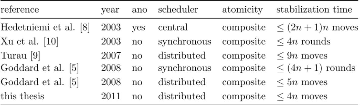
A good survey for the self-stabilizing algorithms is [6]. For convenience, if the stabi-lization time of a self-stabilizing algorithm is at most t moves (resp., rounds), then we say it is a t-move (resp., t-round) algorithm. The followings are self-stabilizing algorithms for the MDS problem. In 2003, Hedetniemi et al. proposed a (2n + 1)n-move algorithm under central scheduler [8]. In 2003, Xu et al. proposed a 4n-round algorithm under synchronous scheduler [10]. In 2007, Turau proposed a 9n-move algorithm under a dis-tributed scheduler [9]. Later, in 2008, Goddard et al. proposed a (4n+1)-round algorithm under synchronous scheduler; the same algorithm becomes a 5n-move algorithm if under a distributed scheduler [5].
It is a challenge to develop an algorithm that takes less than 5n moves under a dis-tributed scheduler. The purpose of this thesis is to propose such an algorithm. In par-ticular, we propose a 4n-move algorithm under a distributed scheduler; an example such that our algorithm takes 4n− 1 moves to reach a legitimate configuration has also been proposed. Our algorithm uses composite atomicity and it requires the local distinct id property, that is, two neighboring nodes must have distinct id’s. We now summarize known results in Table 1 (in this table, “ano” means “the system is anonymous”, where a system is anonymous if the nodes do not have any id).
Table 1: Self-stabilizing minimal dominating set algorithms.
reference year ano scheduler atomicity stabilization time Hedetniemi et al. [8] 2003 yes central composite ≤ (2n + 1)n moves Xu et al. [10] 2003 no synchronous composite ≤ 4n rounds
Turau [9] 2007 no distributed composite ≤ 9n moves
Goddard et al. [5] 2008 no synchronous composite ≤ (4n + 1) rounds Goddard et al. [5] 2008 no distributed composite ≤ 5n moves this thesis 2011 no distributed composite ≤ 4n moves
our main result. The concluding remarks are in the last section.
2
Related works
A good survey for self-stabilizing algorithms for DS, MDS, and other related problems can be found in [6]. In this section, we will briefly review the algorithms in [9] and [5].
The algorithm proposed by Turau in [9] in 2007 is the first self-stabilizing algorithm for solving the MDS problem that stabilizes in linear time under under a distributed scheduler. Turau’s algorithm is a 9n-move algorithm and it makes the assumption that every node has a globally unique id. In the algorithm, each node has a state variable with three choices: OUT, WAIT, and IN. A node has the state OUT (resp., WAIT and resp., IN) if it has a small (resp., median and resp., high) possibility of being a member of the MIS. Let OUT, WAIT, and IN also denote the set of nodes with state OUT, WAIT, and IN, respectively.
Turau first proposed a self-stabilizing algorithm for solving the MIS problem and then, extended the algorithm to solve the MDS problem. The algorithm for solving the MIS problem operates according the the following rules: (r-1) a node in OUT will move to WAIT if none of its neighbors is in IN; (r-2) a node in WAIT will move to OUT if it has a neighbor in IN; (r-3) a node in WAIT will move to IN if none of its neighbors is in IN and none of its neighbors is in WAIT and has a lower id; (r-4) a node in IN will move
to OUT if it has at least one neighbor in IN. Turau extended the MIS algorithm to solve the MDS problem as follows. Each node has an additional variable, called pointer, and will adjust its pointer as follows: (1) a node that will move from WAIT to IN changes its pointer to null; (2) a node in IN adjusts its pointer to null; (3) a node in OUT that has a unique in-neighbor (say, w); (4) a node in OUT that has at least two neighbors in IN adjusts its pointer to null. Besides, rule (r-4) is modified as: a node in IN will move to OUT if it has at least one neighbor in IN and it has no neighbor pointing to it.
In [5], Goddard et al. proposed a 5n-move algorithm for the MDS problem. They assume nodes having locally distinct id’s and assume a distributed scheduler. Each node has a Boolean variable indicating whether it belongs to the set IN and an integer variable indicating the number of neighbors that are in the set IN. A node is allowed to join the set IN if it has no neighbors in IN, its integer variable is 0, and its id is the lowest one among these neighbors with integer variable 0 and itself. On the other hand, a node is allowed to leave the set IN if it has no neighbors in IN and every neighbor which is not in IN has more than one neighbors in IN.
3
Our main result
The purpose of this section is to propose our main result, a self-stabilizing 4n-move algorithm for the MDS problem using a distributed scheduler.
3.1
Our algorithm
In our algorithm, each node has a local distinct (within its neighborhood) id, a variable called state, and a variable called dependent. Let v be a node. The value of v.state is either IN or OUT, where IN (resp., OUT) means that v is (resp., is not) in the MDS. We
will also use IN and OUT to denote the set of nodes with state IN and OUT, respectively. The value of v.dependent is either 0 or the id of a neighbor of v or Λ. In particular, if v has no neighbor in IN, then v.dependent is set to 0; if v has a unique neighbor in IN, then v.dependent is set to the id of this neighbor; if v has more than one neighbor in IN, then v.dependent is set to Λ.
Let v and w be two nodes. For convenience, we use v ∼ w to denote “v is adjacent to w”. If v ∼ w and v.state = IN, then v is called an in-neighbor of w; on the other hand, if v ∼ w and v.state = OUT, then v is called a out-neighbor of w. For each node v, we also define Boolean variables v.inNeighbor, v.independentNeighborWithLowerID, v.dependentOutNeighbors, and v.moreThanOneInNeighbor as follows (note that≡ denotes “is defined as” and∧ denotes “and”).
• v.inNeighbor ≡ v has an in-neighbor;
• v.independentNeighborWithLowerID ≡ ∃ w ∼ v such that w.dependent = 0 ∧ w.id < v.id;
• v.dependentOutNeighbors ≡ ∃ an out-neighbor w of v such that w.dependent = v; • v.moreThanOneInNeighbor ≡ v has more than one in-neighbor.
For each node v, we also an additional predicate
• v.uniqueInNeighbor(w) ≡ v has a unique in-neighbor and it is w.
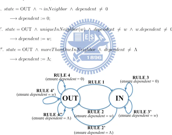
Our self-stabilizing algorithm uses the following rules. In these rules, ¬ denotes “not” and := denotes “is assigned the value”. The state diagram of our algorithm is shown in Figure 1.
1. state = OUT∧ ¬ inNeighbor ∧ dependent = 0 ∧ ¬ independentNeighborW ithLowerId −→ state := IN;
2. state = IN ∧ uniqueInNeighbor(w) ∧ ¬ dependentOutNeighbors −→ state := OUT; dependent := w;
2′. state = IN ∧ moreT hanOneInNeighbor ∧ ¬ dependentOutNeighbors −→ state := OUT; dependent := Λ;
3. state = IN ∧ ¬ inNeighbor ∧ dependent ̸= 0 −→ dependent := 0;
3′. state = IN ∧ uniqueInNeighbor(w) ∧ dependent ̸= w −→ dependent := w;
4. state = OUT ∧ ¬ inNeighbor ∧ dependent ̸= 0 −→ dependent := 0;
4′. state = OUT ∧ uniqueInNeighbor(w) ∧ dependent ̸= w ∧ w.dependent ̸= 0 −→ dependent := w;
4′′. state = OUT ∧ moreT hanOneInNeighbor ∧ dependent ̸= Λ −→ dependent := Λ;
OUT
IN
RULE 1 RULE 2 RULE 2’ RULE 3 RULE 3’ RULE 4 RULE 4’’ RULE 4’ (ensure dependent = 0) (ensure dependent = 0) (ensure dependent !) (ensure dependent !) (ensure dependent w) (ensure dependent w) (ensure dependent w)Figure 1: The state diagram of our algorithm.
The value of dependent will be set according to the rule executed. As an example, if rule 2 is executed, then the value of dependent is set to w, which equals to the value of
the parameter w stored in uniqueInNeighbor.
3.2
Correction and convergence
To prove the correctness of our algorithm, we first prove that when each node has no enabled rules, the set of nodes with state IN form a minimal dominating set.
Theorem 3.1. When each node has no enabled rules, the set D ={v | v.state = IN} is a minimal dominating set of G.
Proof. Suppose to the contradiction that D is not a minimal dominating set of G. Then D is not a dominating set or D is a dominating set but not a minimal one. First consider the case that D is not a dominating set. In this case, there must exist a node /∈ D that has no in-neighbors. Thus
S ={v ̸∈ D | w.state ̸= IN ∀w ∈ N(v)} ̸= ∅.
Since rule 4 is not enabled, we have v.dependent = 0 for all v ∈ S. Choose v0 from S such that v0 is the node with the smallest id in S; since S ̸= ∅, v0 exists. Then v0 satisfies all the constraints of rule 1; rule 1 can be enabled. This contradicts with the assumption that each node has no enabled rules.
Now consider the case that D is a dominating set but not a minimal one. Then there exists a node v ∈ D such that v has in-neighbors and every out-neighbor w of v has at least two in-neighbors. For each such w, w.state is OUT and w.moreT hanOneInN eighbor is true. Since Rule 4′′ is not enabled, we must have w.dependent = ∧. But, for node v, either rule 2 or rule 2′ could be enabled; if v has a unique in-neighbor, then rule 2 could be enabled and if v has more than one in-neighbor, then rule 2′ could be enabled. Again, this contradicts with the assumption that every node has no enabled rules.
We now use Lemmas 3.2, 3.3, 3.4, 3.5 and Theorem 3.6 to prove that our algorithm stabilizes after at most 4n moves under a distributed scheduler.
Lemma 3.2. No two neighboring nodes will execute rule 1 at the same time. Proof. This lemma follows from the locally distinct id property.
Lemma 3.3. After a node v executes rule 1, v will not execute any other rules.
Proof. Since v executes rule 1, v has no in-neighbors and v.dependent = 0 before it executes rule 1. Since v has no in-neighbors, for all w ∈ N(v), we have w.state is OUT before v executes rule 1. By Lemma 3.2, for all w ∈ N(v), w.state remains OUT after v executes rule 1. Thus after v executes rule 1, v.state becomes IN and the only rules that v can execute are: rules 2, 2′, 3, and 3′. We have two claims.
Claim 1: v cannot execute rules 2, 2′, and 3′.
Proof of Claim 1. Recall that v has no in-neighbors before it executes rule 1. Thus for all w∈ N(v), we have w.state is OUT before v executes rule 1. After the execution of rule 1, if v executes rule 2 or 2′ or 3′, then v must have a neighbor (say, w) such that w.state is changed from OUT to IN. Notice that rules 4, 4′, and 4′′ will not change the state of a node. Thus w.state can be changed from OUT to IN only by the execution of rule 1. This is impossible; since if w can execute rule 1, then w.inN eighbor has to be false but w already has a neighbor v such that v.state is IN. Therefore w cannot execute rule 1. Consequently, v cannot execute rules 2, 2′, and 3′.
Claim 2: v cannot execute rule 3.
Proof of Claim 2. Since v executes rule 1, v.dependent is 0. After the execution of rule 1, v.state becomes IN. For v to execute rule 3, v.dependent cannot be 0. Consequently, v cannot execute rule 3.
Lemma 3.4. After a node v executes rule 3, v will not execute any other rules.
Proof. Since v executes rule 3, v has no in-neighbors before it executes rule 3. Since v has no in-neighbors, for all w ∈ N(v), we have w.state is OUT before v executes rule 3. Since v is a neighbor of w and v.state is IN, w.inN eighbor is true and consequently w cannot execute rules 1. Thus for all w ∈ N(v), w.state remains OUT after v executes rule 3.Thus after v executes rule 3, v.state remains IN and the only rules that v can execute are: rules 2, 2′, 3, and 3′. We have two claims.
Claim 1: v cannot execute rules 2, 2′, and 3′.
Proof of Claim 1. Recall that v has no in-neighbors before it executes rule 3. Thus for all w∈ N(v), we have w.state is OUT before v executes rule 3. After the execution of rule 3, if v executes rule 2 or 2′ or 3′, then v must have a neighbor (say, w) such that w.state is changed from OUT to IN. Notice that rules 4, 4′, and 4′′ will not change the state of a node. Thus w.state can be changed from OUT to IN only by the execution of rule 1. This is impossible; since if w can execute rule 1, then w.inN eighbor has to be false but w already has a neighbor v such that v.state is IN. Therefore w cannot execute rule 1. Consequently, v cannot execute rules 2, 2′, and 3′.
Claim 2: v cannot execute rule 3.
Proof of Claim 2. After v executes rule 3, v.dependent is 0. For v to execute rule 3 next, v.dependent cannot be 0. Consequently, v cannot execute rule 3.
By Claims 1 and 2, we complete this proof.
Lemma 3.5. Suppose v.state is OUT and a neighbor w of v executes rule 1. Then the only rule that v can execute is rule 4′′ and after v executes rule 4′′, v will not execute any other rules.
Proof. Since w executes rule 1, w.inN eighbor is false, w.dependent is 0. By Lemma 3.3, after w executes rule 1, w will not execute any other rules. Thus after w executes rule 1,
w.state remains to be IN. Since w is a neighbor of v and w.state is IN, v.inN eighbor is true and consequently v cannot execute rules 1 and 4. If w is the unique in-neighbor of v, then by the fact that w.dependent is 0, v cannot execute rule 4′. Hence the only rule that v can execute is rule 4′′. Suppose that v executes rule 4′′. Then v.dependent is set to Λ; as a result, v will not execute any other rules.
Theorem 3.6. Our algorithm is a self-stabilizing algorithm for the minimal dominating set problem under a distributed scheduler. Furthermore, it stabilizes after at most 4n moves.
Proof. By Theorem 3.1, our algorithm is a self-stabilizing algorithm for the minimal dominating set problem. It remains to prove that our algorithm stabilizes after at most 4n moves under a distributed scheduler. We will prove this by showing that each node v takes at most 4 moves under a distributed scheduler.
LetI = {1, 2, 2′, 3, 3′, 4, 4′, 4′′}, i.e., I is the set containing all the indices of the rules of our algorithm. Let k be a positive integer and let r1, r2, . . . , rk ∈ I (note that r1, r2, . . . , rk
are not necessarily distinct). The sequence < r1, r2, . . . , rk > is called a move sequence of
v if v can execute rule r1, then execute rule r2, . . ., and then rule rk. The number k is
called the length of the move sequence. A move sequence of v is a longest move sequence if its length is the largest among all the move sequences of v. Let l∗ denote the length of a longest move sequence of v for convenience. Initially, v.state is either IN or OUT.
Suppose initially v.state is OUT. Then the only rules that v can execute are 1, 4, 4′ and 4′′. According the rule that v executes, there are four cases.
(i) v executes rule 1. Then by Lemma 3.3, l∗ = 1.
(ii) v executes rule 4. After the execution, v.state remains OUT. Thus the next rules that v can execute are 1, 4, 4′ and 4′′. We have four sub-cases.
(ii-1) If the next rule executed by v is rule 1, then by Lemma 3.3, l∗ = 2. (ii-2) It is impossible that the next rule executed by v is still rule 4.
(ii-3) We claim that it is also impossible that the next rule executed by v is rule 4′. The reason is as follows. Before v executes rule 4 for the first time, v.inN eighbor is false; therefore, w.state is OUT for all w ∈ N(v). For v to execute rule 4′, one of the neighbors of v (say, w) has to change its state from OUT to IN. But w can change its state from OUT to IN only by executing rule 1. By Lemma 3.5, the only rule that v can execute is rule 4′′.
(ii-4) Before v executes rule 4, v.inN eighbor is false and therefore w.state is OUT for all w∈ N(v). Suppose that the next rule executed by v is rule 4′′. For v to execute rule 4′′, at least two of the neighbors of v have to change their state from OUT to IN. Let w be one of such neighbors. Note that w can change its state from OUT to IN only by executing rule 1. By Lemma 3.5, we know that the only rule that v can execute is rule 4′′ and after v executes rule 4′′, v will not execute any other rules. Thus l∗ = 2.
(iii) v executes rule 4′. After the execution, v.state remains OUT. Thus the next rules that v can execute are 1, 4, 4′ and 4′′. We have four sub-cases.
(iii-1) If the next rule executed by v is rule 1, then by Lemma 3.3, l∗ = 2.
(iii-2) If the next rule executed by v is rule 4, then by (ii), we know that the longest move sequence is < 4′, 4, 1 > or < 4′, 4, 4′′>; thus l∗ = 3.
(iii-3) We claim that it is impossible that the next rule executed by v is still rule 4′. The reason is as follows. Before v executes rule 4′ for the first time, v has a unique in-neighbor w and v.dependent is set to w after the execution of rule 4′. If the next rule executed by v is still rule 4′, then we must have v.dependent not equal to the unique in-neighbor of v. Thus w has to change
its state from IN to OUT and another neighbor (say, x) of v has to change its state from OUT to IN. Moreover, x must become the unique in-neighbor of v and x.dependent ̸= 0 must occur so that the next rule executed by v can be rule 4′. Note that x can change its state from OUT to IN only by executing rule 1. However, for x to execute rule 1, x.dependent = 0 must occur; this contradicts with the assumption that x.dependent ̸= 0 must occur. Thus it is impossible that the next rule executed by v is still rule 4′.
(iii-4) Before v executes rule 4′′, v has a unique in-neighbor. Suppose that the next rule executed by v is rule 4′′. For v to execute rule 4′′, at least one of the neighbors of v has to change its state from OUT to IN. Let w be such a neighbor. Note that w can change its state from OUT to IN only by executing rule 1. By Lemma 3.5, we know that the only rule that v can execute is rule 4′′ and after v executes rule 4′′, v will not execute any other rules. Thus l∗ = 2. (iv) v executes rule 4′′. After the execution, v.state remains OUT. Thus the next rules
that v can execute are 1, 4, 4′ and 4′′. Again, we have four sub-cases. (iv-1) If the next rule executed by v is rule 1, then by Lemma 3.3, l∗ = 2.
(iv-2) If the next rule executed by v is rule 4, then by (ii), we know that the longest move sequence is < 4′′, 4, 1 > or < 4′′, 4, 4′′>; thus l∗ = 3.
(iv-3) If the next rule executed by v is rule 4′, then by (iii), we know that the longest move sequence is < 4′′, 4′, 4, 1 > or < 4′′, 4′, 4, 4′′ >; thus l∗ = 4.
(iv-4) It is impossible that the next rule executed by v is still rule 4′′.
Now, suppose initially v.state is IN. Then the only rules that v can execute are 2, 2′, 3 and 3′. According the rule that v executes, there are four cases.
that v can execute are 1, 4, 4′ and 4′′. We have four sub-cases.
(a-1) If the next rule executed by v is rule 1, then by Lemma 3.3, l∗ = 2.
(a-2) If the next rule executed by v is rule 4, then by the above (ii), the longest move sequence is < 2, 4, 1 > or < 2, 4, 4′′ >; thus l∗ = 3.
(a-3) We claim that it is impossible that the next rule executed by v is rule 4′. The reason is as follows. Before v executes rule 2, v has a unique in-neighbor w and v.dependent is set to w after the execution of rule 2. If the next rule executed by v is rule 4′, then we must have v.dependent not equal to the unique in-neighbor of v. Thus w has to change its state from IN to OUT and another neighbor (say, x) of v has to change its state from OUT to IN. Moreover, x must become the unique in-neighbor of v and x.dependent ̸= 0 must occur so that the next rule executed by v can be rule 4′. Note that x can change its state from OUT to IN only by executing rule 1. However, for x to execute rule 1, x.dependent = 0 must occur; this contradicts with the assumption that x.dependent̸= 0 must occur. Thus it is impossible that the next rule executed by v is rule 4′.
(a-4) Before v executes rule 4′′, v has a unique in-neighbor. Suppose that the next rule executed by v is rule 4′′. For v to execute rule 4′′, at least one of the neighbors of v has to change its state from OUT to IN. Let w be such a neighbor. Note that w can change its state from OUT to IN only by executing rule 1. By Lemma 3.5, we know that the only rule that v can execute is rule 4′′ and after v executes rule 4′′, v will not execute any other rules. Thus l∗ = 2. (b) v executes rule 2′. After the execution, v.state becomes OUT. Thus the next rules
that v can execute are 1, 4, 4′ and 4′′. We have four sub-cases.
(b-2) If the next rule executed by v is rule 4, then by (ii), we know that the longest move sequence is < 2′, 4, 1 > or < 2′, 4, 4′′>; thus l∗ = 3.
(b-3) If the next rule executed by v is rule 4′, then by (iii), we know that the longest move sequence is < 2′, 4′, 4, 1 > or < 2′, 4′, 4, 4′′ >; thus l∗ = 4.
(b-4) It is impossible that the next rule executed by v is rule 4′′. (c) v executes rule 3. By Lemma 3.4, l∗ = 1.
(d) v executes rule 3′. After the execution, v.state remains IN. Thus the next rules that v can execute are rules 2, 2′, 3 and 3′. We have four sub-cases.
(d-1) If the next rule executed by v is rule 2, then by (a), the longest move sequence is < 3′, 2, 4, 1 > or < 3′, 2, 4, 4′′ >; thus l∗ = 4.
(d-2) We claim that it is impossible that the next rule executed by v is still rule 2′. The reason is as follows. After the execution of rule 3′, if v executes rule 2′, then v must have a neighbor (say, w) such that w.state is changed from OUT to IN. Notice that rules 4, 4′, and 4′′ will not change the state of a node. Thus w.state can be changed from OUT to IN only by the execution of rule 1. This is impossible; since if w can execute rule 1, then w.inN eighbor has to be false; however, w already has a neighbor v such that v.state is IN. Therefore w cannot execute rule 1. Consequently, v cannot execute rules 2′.
(d-3) If the next rule executed by v is rule 3, then by (c), we know, l∗ = 2.
(d-4) We claim that it is impossible that the next rule executed by v is still rule 3′. The reason is as follows. Before v executes rule 3′ for the first time, v has a unique in-neighbor w and v.dependent is set to w after the execution of rule 3′. If the next rule executed by v is still rule 3′, then we must have v.dependent not equal to the unique in-neighbor of v. Thus w has to change its state from
IN to OUT and another neighbor (say, x) of v has to change its state from OUT to IN. Notice that rules 4, 4′, and 4′′ will not change the state of x. Thus x.state can be changed from OUT to IN only by the execution of rule 1. This is impossible; since if x can execute rule 1, then x.inN eighbor has to be false but x already has a neighbor v such that v.state is IN. Therefore x cannot execute rule 1. Thus it is impossible that the next rule executed by v is still rule 3′.
From the above, each node v takes at most 4 moves under a distributed scheduler and we have this theorem.
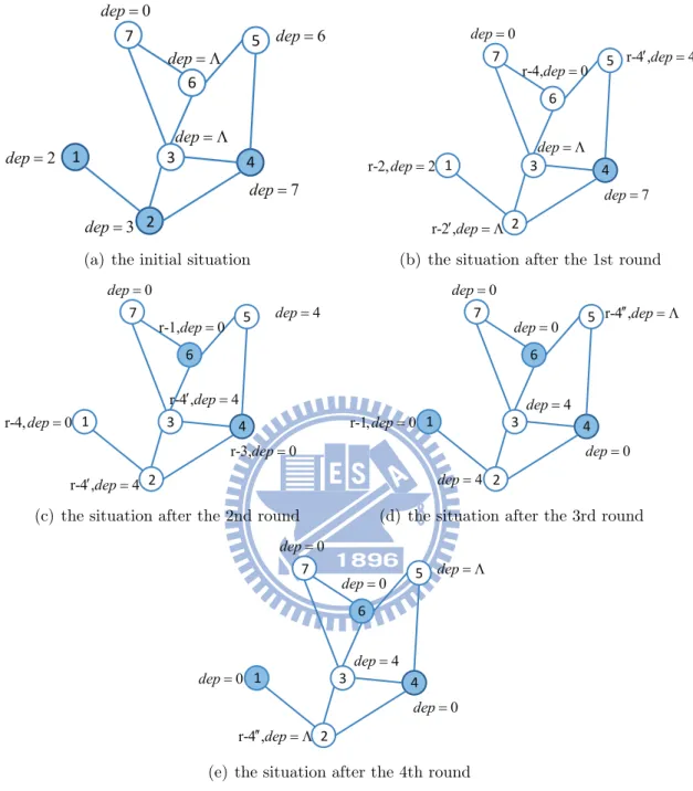
We now give an example of our algorithm; see Figure 2 for an illustration.
In Figure 2, a node colored blue means that this node has state = IN. Also, each node has two tags associated with it: r-k and dep = i, where r-k denotes the rule that is executed by this node and dep = i means that the value of dependent is i. See Figure 2(a). Initially nodes 1, 2, and 4 have state = IN. However, {1, 2, 4} does not form a minimal dominating set. Moreover, the value of dependent of nodes 2, 4, 5 and 6 are incorrect. In Figure 2(b), we see that node 1 executes rule 2, node 2 executes rule 2′, node 5 executes rule 4′, and node 6 executes rule 4. In Figure 2(c), we see that nodes 1, 2, 3, 4, and 6 execute rules 4, 4′, 4′, 3, and 1, respectively. In Figure 2(d), we see that nodes 1 and 5 execute rules 1 and 4′′, respectively. In Figure 2(e), we see that after node 2 executes rule 4′′, no node will be enabled. Finally nodes 1, 4 and 6 have state = IN and in total 12 moves are executed. It is clear that{1, 4, 6} is a minimal dominating set.
7 dep 3 dep 2 dep 1 2 3 4 5 6 7 dep 6 0 dep dep ! dep !
(a) the initial situation
7 dep r-2 ,dep! " r-2,dep 2 1 2 3 4 5 6 7 r-4 ,dep!4 0 dep r-4,dep 0 dep !
(b) the situation after the 1st round
r-3,dep 0 r-4 ,dep!4 r-4,dep 0 1 2 3 4 5 6 7 dep 4 0 dep r-1,dep 0 r-4 ,dep!4
(c) the situation after the 2nd round
0 dep 4 dep r-1,dep 0 1 2 3 4 5 6 7 r-4 , dep! " 0 dep 0 dep 4 dep
(d) the situation after the 3rd round
0 dep r-4 , dep! " 0 dep 1 2 3 4 5 6 7 dep ! 0 dep 0 dep 4 dep
(e) the situation after the 4th round
4
Concluding remarks
In this thesis, we propose an efficient self-stabilizing algorithm for solving the minimal dominating set (MDS) problem. This algorithm is a 4n-move algorithm and it outperforms the best known algorithm, which is a 5n-move algorithm. We are curious about whether there is still a better algorithm than the proposed one.
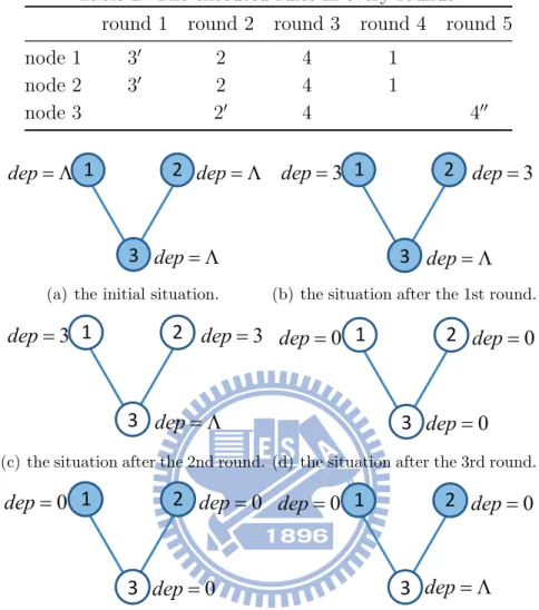
Before ending this thesis, we propose an example such that our algorithm takes 4n− 1 moves to reach a legitimate configuration. Consider a distributed system with 3 nodes in which node 1 and node 2 are adjacent to node 3; see Figure 3. Note that in this figure, dep is the abbreviation of dependent. Note that a node colored blue means that its state = IN, and a node colored white means that its state = OUT.
Assume that the id’s of these three nodes are 1, 2, and 3. The executed rules of each node for every round are shown in Table. 2. Initially all nodes have state = IN and have dependent being null. The scheduler selects nodes 1 and 2 to execute rule 3′ in the first round, then the value of each of their dependent becomes 3. In the second round, the scheduler selects nodes 1 and 2 to execute rule 2 and it selects node 3 to execute rule 2′ (their state become OUT). In the third round, the scheduler selects all of the nodes to execute rule 4; therefore the value of dependent is 0. Finally, the scheduler selects nodes 1 and 2 for executing rule 1 in the fourth round (their states become IN), and selects node 3 executing rule 4′′. The above progress is depicted in Figure 3.
In fact, we can generalize this case. Consider a distributed system with n nodes in which node 1, node 2,..., and node n− 1 are adjacent to node n; the initial state variable, initial dependent variable, and the action of nodes n is the same as these of node 3 in the case of 3 nodes. The initial state variable, initial dependent variable, and the action of the other nodes is the same as these of node 1 in the case of 3 nodes.
Table 2: The executed rules in every rounds. round 1 round 2 round 3 round 4 round 5
node 1 3′ 2 4 1 node 2 3′ 2 4 1 node 3 2′ 4 4′′ 1 3 2 dep ! dep ! dep !
(a) the initial situation.
1 3 2 dep ! 3 dep 3 dep
(b) the situation after the 1st round.
1
3
2
dep !
3
dep
3
dep
(c) the situation after the 2nd round.
1
3
2
0
dep
0
dep
0
dep
(d) the situation after the 3rd round.
1
3
2
0
dep
0
dep
0
dep
(e) the situation after the 4th round.
1
3
2
dep !
0
dep
0
dep
(f) the situation after the 5th round.
Figure 3: An example such that our algorithm takes 4n− 1 moves to reach a legitimate configuration.
References
[1] E. W. Dijkstra, Self-stabilizing systems in spite of distributed control, Communica-tion of the ACM 17 (11) (1974) 643-644.
[2] S. Dolev, Self-stabilization, MIT Press, 2000.
[3] S. Dolev, A. Israeli, and S. Moran, Self-stabilization of dynamic systems assuming only read/write atomicity, Distributed Computing 7 (1) (1993) 3-16.
[4] W. Goddard, S. T. Hedetniemi, D. P. Jacobs, and P. K. Srimani, A self-stabilizing distributed algorithm for minimal total domination in an arbitrary system graph, in: Proc. 17th International Parallel and Distributed Processing Symposium, 2003. [5] W. Goddard, S. T. Hedetniemi, D. P. Jacobs, P. K. Srimani, and Z. Xu,
Self-stabilizing graph protocols, Parallel Processing Letters 18 (1) (2008) 189-199. [6] N. Guellati and H. Kheddouci, A survey on self-stabilizing algorithms for
indepen-dent, domination, coloring, and matching in graphs, Journal Parallel and Distributed Computing 70 (4) (2010) 406-415.
[7] T. W. Haynes, S. T. Hedetniemi, and P. J. Slater, Fundamentals of Domination in Graphs, Marcel Dekker, 1998.
[8] S. M. Hedetniemi, S. T. Hedetniemi, D. P. Jacobs, and P. K. Srimani, Self-stabilizing algorithms for minimal dominating sets and maximal independent sets, Computer Mathematics and Applications 46 (5-6) (2003) 805-811.
[9] V. Turau, Linear self-stabilizing algorithms for the independent and dominating set problems using an unfair distributed scheduler, Information Processing Letters 103 (3) (2007) 88-93.
[10] Z. Xu, S. T. Hedetniemi, W. Goddard, and P. K. Srimani, A synchronous self-stabilizing minimal domination protocol in an arbitrary network graph, in: Proc. 5th International Workshop on Distributed Computing, 2003.