國
立
交
通
大
學
資訊科學與工程研究所
碩
士
論
文
對 交 通 資 料 之 混 合 式 預 測 演 算 法
A Hybrid Prediction Algorithm for Traffic Speed Data
Prediction
研 究 生:黃柏崴
對交通資料之混合式預測演算法
A Hybrid Prediction Algorithm for Traffic Speed Data Prediction
研 究 生:黃伯崴 Student:Bo-Wei Huang
指導教授:彭文志 Advisor:Wen-Chih Peng
國 立 交 通 大 學
資 訊 科 學 與 工 程 研 究 所
碩 士 論 文
A ThesisSubmitted to Institute of Computer Science and Engineering College of Computer Science
National Chiao Tung University in partial Fulfillment of the Requirements
for the Degree of Master
in
Computer Science
June 2012
Chinese Abstract
有許多類型的數據可以被視為作為時間序列。因此,時間序列的預測被應用在各種不同的領域, 如投資,交通預測等,交通狀態預測可用於擁塞避免和旅遊規劃。我們要解決的問題是利用時 間序列預測來對交通狀況進行預測。時間序列的預測問題定義如下,給予一查詢時間,及時間 序列數據,預測出在查詢時間的值。通常情況下,查詢時間為未來的時間。在這篇論文中,我 們 提 出 了 一 個 混 合 式 預 測 算 法 , 同 時 利 用 基 於 回 歸(regression-based) 和 基 於 分 群 (clustering-bsaed)的預測方法。明顯地,基於回歸的預測在預測時間離目前時間不會太遠時, 有較準確的預測結果,而基於分群的預測則在預測時間較遠時有較準確的預測結果。我們觀察 到在時間序列中有一些相似形狀或趨勢。為了捕捉這些形狀,我們利用了分群的概念。從這些 叢集中,我們可以進一步發現他們在時序上的關係。因此,如果查詢時間距離目前時間較遠, 我們利用上述叢集的時序關係,預測可能出的叢集。再從可能出現的叢集中,預測在查詢時間 點上的數據值。在這邊需要注意的是混合了上述兩種方法的混合式演算法使用一個閾值來決定 使用哪種方法。如果查詢時間和當前時間之間的時間差小於閾值,混合預測演算法使用基於回 歸預測。反之,則使用基於分群的預測。為了驗證我們提出的方法,我們進行了大量對真實數 據的實驗。並經由實驗結果證明我們所提出的方法既準確又實用。Abstract
Many types of data can be regarded as time series data. Therefore time series data predictions are applied in a wide range of domains, such as investment, traffic prediction, etc. Traffic status prediction can be used for congestion avoidance and travel planning. We solve the problem of predicting traffic status by time series prediction. The time series data prediction problem is that given a query time and time series data, we intend to predict the data value at the query time. Usually, a query time will be a future time. In this paper, we propose a hybrid prediction algorithm which exploits regression-based and clustering-based prediction methods. Explicitly, regression-based prediction is accurate when the query time is not too far from the current time. Note that time series data may have some similar shapes or trends. To capture the similar shapes hidden in this data, we utilize clustering concepts. Using these clusters, we could further discover their sequential relationships. As such, if the query time is far away from the current time, we utilize the above cluster sequential relationships to predict the possible similar cluster. From the similar cluster, the data value at the query time is obtained. Note that the hybrid algorithm aggregates the above two methods using one threshold that decides which method to use. If the time difference between the query time and the current time is smaller than the prediction length threshold, hybrid prediction uses regression-based prediction. Otherwise, our hybrid algorithm uses clustering-based prediction. To prove our proposed methods, we have carried out a set of experiments on real data sets to compare the accuracy of the methods. The results of the experiments prove that our proposed methods are both accurate and practical.
Acknowledgement
本篇研究論文的完成,首先需感謝我的父母,有父母對我的支持,我才能在研究所一直堅持 下去,沒有父母也不會有今天的我。接著是這兩年來一路指導我的指導教授彭文志,彭文志 教授一直是個很關心學生,很尊重學生意見的好老師。另外也感謝擔任本論文口試委員的陳 伶志與葉彌妍院士給予寶貴的意見。 能夠完成這篇論文還要感謝實驗室同學的協助,文圓學長給了很多機器管理上的協助,綾音 學姊和孟芬學姊在論文的寫作上給了很多建議。同屆的堃瑋與雅婷與我一起參予了與英業達 的合作計畫,在計畫中多虧了兩位同學的協助才能順利將計畫完成。宇綸和依琴則是在實驗 室和我們一起完成了很多的事情。還有實驗室的學弟妹們,感謝你們在口試的時候協助採買 口試用的點心水果等,使得口試可以更順利的進行。 最後還要感謝我的室友們以及網路上認識的朋友,智焙一直以來在論文以及生活上提供了相 當多的協助,陪我進行了多次口試的演練以及尋找工作上的意見。珉誠提供了交通工具讓我 們這幾個室友有機會到處品嘗新竹的美食,並且讓我更加體會到生命的可貴。在實驗室機器 故障的時候,珉誠與建安給了不少幫助,讓我學習到了不少機器管理的技術。網路上認識的 朋友們陪我經歷了一場又一場的冒險,讓我在閒暇之餘有一個可以宣洩壓力的管道。如果沒 有你們這些好朋友,相信我今天也沒辦法完成這篇論文。 最後,感謝所有曾經協助過我的人,你們使得這篇論文更加的完美,謝謝你們。Contents
Chinese Abstract I English Abstract II Acknowledgements III Contents IV List of Figures VI 1 Introduction 1 2 Related Work 5 3 Preliminaries 8 3.1 Problem Definition . . . 9 4 Prediction Methods 11 4.1 Regression . . . 11 4.2 Clustering-based prediction . . . 13 4.2.1 Scheme MCF . . . 15 4.2.2 Scheme MPST . . . 16 4.3 Hybrid prediction . . . 20 5 Performance Evaluation 21 6 Future Work 28List of Figures
1.1 An example of time series: traffic speed . . . 1
3.1 Prediction for traffic status . . . 10
4.1 Clustering-based prediction flow chart . . . 14
4.2 An example of PST . . . 17
5.1 Prediction results for short-term prediction . . . 22
5.2 Prediction results for long-term prediction . . . 22
5.3 Prediction results for 6 hours continuous prediction . . . 22
5.4 Comparison average trace length of MPST and ECTS . . . 23
5.5 Different periods for MCF . . . 24
5.6 Different periods for MPST . . . 24
5.7 Different tree heights for MPST . . . 24
5.8 Different pattern similarity threshold for MPST . . . 25
5.9 Different threshold for Hybrid Prediction . . . 26
Chapter 1
Introduction
With the e-revolution, many businesses and organizations are now generating massive amounts of data which are constituted of values and time [16]. We call these data sets time series data. Therefore time series data predictions are applied in many domains, such as stock control, sales forecasting, financial risk management, traffic prediction, weather reporting, etc [2]. Time series data can be categorized as either univariate or multivariate time series. A classical univariate time series is shown in Fig. 1.1. This example shows the average traffic speeds of one highway segment. In this paper, we want to predict the speed value in the future.
The common application of traffic status prediction is congestion avoidance. We can know which roads experience traffic jams from the prediction results, and then we can take a road
30 35 40 45 50 55 60 65 70 0 10 20 30 40 50 Speed(km/hr) Time(min) Traffic Speed Sequence
Traffic Speed
that is not congested. This technique can also be used in navigation. The navigation algorithm can consider the predicted traffic status, and can thus find a faster route. To predict the traffic status in the future, we must know the features of the traffic status data. It is almost a regular curve every day. The rising and falling of traffic speed results from human behavior, and the heaviest traffic flow is due to commuting which occurs on weekdays. Another important feature of traffic status data we observed is that congestion will not happen suddenly, as while it is happening, the traffic speed slows down gradually. Therefore, traffic status can be predicted by both short-term and long-term prediction methods.
There are many existing works about time series data analysis. Time series analysis can be categorized as: description, modeling, forecasting, and control [2], of which we focus on time series forecasting, a.k.a. time series prediction, in this work. In the domain of time series forecasting, some works are accurate in short-term prediction but inaccurate in long-term prediction [19], while others are vice versa [23]. Many methods can be used to predict time series values, but they are generally designed for specific situations, so they cannot process all types of data with high performance. For example, the method used to predict traffic cannot be applied to stocks because the average value of traffic will not change with time, but stocks will. Therefore we have improved the accuracy of these methods using a combination technique.
In this work, we want to predict the value of traffic status in the future. To simplify our problem, we only focus on traffic speed. Assume that the traffic status data have patterns resulting from human behavior. Our proposed method can discover the patterns, and use these patterns to predict the time series value.
However, we do not focus on one of the applications. Thus we should solve the requirement using both short-term and long-term prediction. For example, short-term prediction is needed while driving on the road, and long-term prediction is needed while planning travel. Therefore we should deal with the disadvantages of both short-term and long-term prediction.
In this paper, we propose a hybrid prediction algorithm for time series data. This algorithm explores two types of prediction methods: regression-based and clustering-based. Regression-based prediction uses linear regression to construct the prediction model for a time series. This method is only accurate when the query time is close to the current time because regression-based prediction can only construct a linear model. The linear model goes farther and further
from the time series with increasing time. For example, if a linear model of predicting traffic status is a decreasing line, the predicted value is a minus value when the query time is far away from the current time. However, a minus value for speed is not reasonable. Clustering-based prediction is a long-term prediction method because it uses subsequence of time series as its prediction unit. When using a clustering algorithm as a prediction method, however, some issues should be considered. These issues include: sequence segmenting, similarity function, clustering algorithm, and prediction method. The input time series data should be segmented before clustering because a single sequence cannot be clustered. Then, the clustering algorithm aggregates the similar sequences into a cluster according to the similarity function. The choice of clustering algorithm is important because different algorithms generate extremely different clusters. Finally the clusters can be used to predict values, including how to find frequent pattern and how to predict the value. However, clustering-based prediction methods are not more accurate than regression-based methods when the query is close to the current time. Thus, we propose a hybrid prediction method that exploits different prediction methods to avoid the disadvantages of previous approaches.
In the hybrid prediction method , different prediction methods are used according to different parameters. Linear regression is used for short-term prediction because it can make precise prediction when the query time is not too far from the current time. For long-term predictions, we use based prediction methods. The reason for choosing clustering-based prediction methods is that the data results from human behaviors are periodic. For example, people need to sleep every day, so obviously the loading of servers that provide services for humans is heavier in the daytime, which is a periodic pattern of resource utility for servers. Another example is that some people check the news and their e-mails when they get up. In fact the data we collected reflects those behaviors. Clustering methods can be used to aggregate similar time series together. Thus each cluster can be regarded as a pattern of data. Afterwards, we can use these patterns to predict the time series value in the future.
To summarize, the main contributions of this paper are as follows:
• Proposing two clustering-based prediction methods MCF and MPST which can predict
the future values of time series in the long-term
from a regression-based prediction method and a clustering-based prediction method
• Using a clustering method on patterns and using the pattern sequence to predict time
series data
• carrying out performance evaluation of the proposed methods to prove the performance
The rest of this paper is organized as follows. We discuss the existing works and their disadvantages in Section 2. In Section 3, we define our problem and some terms more formally and clearly. In Section 4, we explain how our methods predict the data. In Section 5, we do some experiments to prove that our proposed methods show obvious improvement. Finally, we discuss our future work in Section 6 and summarize the paper in Section 7.
Chapter 2
Related Work
There are many existing works about time series data analysis or prediction. These works can be categorized as: time series prediction and other time series analysis. Works about time series prediction can be further divided into short-term prediction only and both short-term and long-term prediction. Short-term and long-term predictions differ in their accuracy for different prediction lengths. Short-term predictions are greatly affected by prediction length in that their accuracy decreases rapidly with the increase in prediction length.
In [13], [10] and [14], the authors proposed algorithms for finding time series motifs, which is a type of time series analysis. In these works, the definition of time series motif is the nearest pair of subsequences in a long time series. These works focus on how to mkae the computation of finding motif faster; the method is to reduce the number of distance computations. The problem of using motifs as a prediction method, however, is that there is not sufficient support. The motifs are only two subsequences in the time series data logs, so we do not have enough evidence to say that the future value will be similar to the motif.
There are other works about time series prediction but their focuses are not the accuracy of predictions. In [7], the author is solving the bottleneck of time series prediction to do online stream mining. In [18], the author implements an adaptive runtime anomaly prediction system, and in these works the main goal is to improve efficiency. These works are to solve problems for a particular type of data or to improve efficiency, but their methods cannot be used to improve accuracy when predicting different types of time series data.
In [6] and [25], the authors use neural networks to predict the future values of time series. Neural networks can construct a prediction model and do error correction for the model. However they can only predict the next value of a time series. In [22], Wang et al. proposed a two-phase iterative prediction approach which uses the pattern-based hidden Markov model. In these works, the methods can only predict the next state of data. In contrast, our proposed method can predict any prediction length. However, the concept of the hidden Markov model is like our proposed clustering-based prediction method MPST. The difference is that MPST uses subsequences as the prediction unit, while the hidden Markov model uses value as the prediction unit. Thus MPST can predict more than the hidden Markov model.
In [24], Xiong et al. proposed a resource analysis module and a resource allocation module using regression, a regression tree and boosting to analyze the resource usage in a cloud environment. Their approach uses additional information such as memory to predict the CPU usage. But in our problem we only want to use one dimensional time series data logs. Furthermore, this is a regression-based prediction method, so its accuracy is affected by the prediction length.
There are some works for long-term prediction such as [23] and [16]. In [23], Xing et al. proposed a method that classifies time series by prefix, and then calculates how to find the minimal prefix length. We can use this classification method to classify time series and predict the remaining values by the class’s average series. However, this method needs a long prefix, and the required length of the prefix is not a fixed value. Therefore it cannot always give a prediction result, as it cannot make a prediction when the prefix length is not long enough. In [16], Ruta et al. proposed a generic architecture that can generate a prediction model based on any time series prediction method. This method can be short-term or long-term prediction method. It is decided by the method we give to the training process. However, it needs a great amount of time to train many models and to choose better ones to do the combination. In [11], Ha et al. proposed a method to predict stocks. Their prediction is based on data increasing and decreasing. Therefore this method can be used for prediction of data which is affected by increasing and decreasing. However, not all time series data have such a pattern. For example, stocks and temperatures can be predicted using this method, but traffic speed cannot.
series. This problem is called ”symbolic time series analysis” in other works. There are many advantages of symbolization, such as reducing space, noise filtering, and getting more temporal information[17]. The methods of symbolic time series analysis can be categorized into two domains: quantization and temporal segmentation. The main differences between these two domains are the breakpoints. The breakpoints of quantization are in the amplitude domain, while for temporal segmentation they are in the temporal domain. The existing quantization methods include SAX [8] and PERSIST [12]. These methods symbolize the time series by amplitude, but they cannot distinguish the shape of the time series. For example, the increasing and decreasing line can be marked with the same symbol. Therefore these methods cannot be applied to our problem. In the temporal segmentation method ACA [26], Zhou et al. used clustering to symbolize the time series, as we do in this work.
To the best of our knowledge, we are the first to consider the time difference between ”the query time” and ”the current time”. If the query time is close to the current time, a regression method has better accuracy. Furthermore, none of the existing methods we mentioned above can solve this problem. Therefore we propose a hybrid prediction algorithm which exploits both the regression prediction method and the clustering-based prediction method.
Chapter 3
Preliminaries
Before describing our methods, we should define the notations we used and the problem want to solve. In this section we explain the definition of time series, the problem, and issues.
Definition 1 A univariate time series is a sequence of pairs (value,timestamp). The
times-tamps in the sequence are ordered in ascending order, meanings that the time point of the accompanying value is reduced. The values are reduced from continuous data such as traffic status, temperature, or from discrete data such as sales data. We denote xi as the value at
timestamp i in time series x.
For example, a traffic status time series y= {(40, 0), (50, 15), (60, 30), (60, 45)} is a sequence reduced every 15 minutes from a continuous traffic status shown in Fig.1.1. We can present the first value as y0 = 40, the second value as y15 = 50, and other values can be
presented in this way.
Definition 2 A subsequence xi ,j is a subset of x which means the sequence of values from the
time series x which has a timestamp bigger than i and smaller than j in ascending order.
For example, y0 ,30=(40, 50, 60) is a subsequence of y. The time series y= {(40, 0), (50,
15), (60, 30), (60, 45)} can be segmented into two subsequences y0 ,29=(40, 50) and y30 ,45=(60,
Definition 3 Time series period means a time interval within which some pattern in the time
series appears.
We will segment the time series sequence into subsequences by the time series period in our proposed methods. All the segmented subsequences have the same length of the time series
period. For example, the time series z= {(40, 0), (50, 15), (60, 30), (60, 45), (40, 60), (50, 75),
(60, 90), (60, 105)} has a time series period of 45. The pattern (40, 50, 60, 60) appears two times in this time series. Therefore we can segment z into two subsequence z0 ,45 and z46 ,105.
We can find that these two subsequences have the same value sequence. This is why we need to find the time series period and segment the time series.
Definition 4 Prediction length lpredict is the distance from the current time tc to the query
time tq. Therefore, lpredict = tq - tc.
Prediction length is an important parameter in the hybrid prediction method. Many prediction methods have different degrees of accuracy for different prediction lengths.
3.1
Problem Definition
Given a univariate time series data of traffic status S, the current time tc, and the query time
tq, predict the value Stq at the query time tq. To achieve this goal, we assign the training data length ltrain to construct a prediction model. Therefore the total inputs are as follows:
time series data logs S, length of training data ltrain, current time tc and query time tq. The
output is the value at the query time Stq.
Definition 5 Current time tc is the timestamp of the last value of training data S.
For example, given the time series z= {(40, 0), (50, 15), (60, 30), (60, 45), (40, 60), (50, 75), (60, 90), (60, 105)}, the current time tc is 105. In the prediction process, we predict the
value from this time point. In other words, tq should be bigger than tc.
For example, given a time series of traffic status log y= {(40, 0), (50, 15), (60, 30), (60,
30 40 50 60 70 80 90 100 0 10 20 30 40 50 60 Speed(km/hr) Time(min) Traffic Speed Sequence
Real Traffic Speed Training Data Regression Line
(a) Training data length 45
30 40 50 60 70 80 90 100 0 10 20 30 40 50 60 Speed(km/hr) Time(min) Traffic Speed Sequence
Real Traffic Speed Training Data Regression Line
(b) Training data length 15
Figure 3.1: Prediction for traffic status
45 minutes, the predicted speed at time 60 is 70, as shown in Fig.3.1(a). And if the training data length is only 15 minutes, the predicted speed is 60, as shown in Fig.3.1(b). Because when we use 15 minutes training data length, the training sequence is (60,60), we also predict the future values as 60.
Chapter 4
Prediction Methods
We propose three prediction methods in this paper. These methods can be categorized as regression-based, clustering-based and hybrid. In this section, we will explain the reasons for using these methods and their details.
4.1
Regression
The regression-based methods are well-known solutions for finding the nearest polynomial of the log, and are applied in time series analysis. There are some different regression algorithms such as simple linear regression, multiple linear regression, multilevel linear regression and piecewise linear regression.
Simple linear regression is the simplest regression method that can only be used on a univariate time series. Simple regression constructs the regression line, where the sum of the distances between data points and the regression line is the smallest. The formula of the regression line of simple linear regression is shown as Equation 1, where y in the equation means the value and x means the time. The coefficients α and β are to eliminate the sum of the distances between data points and the regression line. For example, Figure 3.1(a) shows two different regression lines that have the smallest distances to the traffic speed log time series.
Multiple linear regression is like simple linear regression, but is used on multivariate time series. Assuming that there are n+1 variables in the time series data, Y is the variable we predict, and X1, X2, ..., Xn are the variables used to predict the value of Y . The formula of
the regression line of multiple linear regression is shown in Equation 2. Yi is the predicted
ith value of variable Y , Xij is the ith observation value of the variable Xj, and ϵi is the ith
independent identically distributed normal error. This method generates a more accurate model but needs many data attributes. However, our problem only focuses on the univariate time series prediction, so we do not need to use multiple linear regression.
Yi = β0+ β1Xi1+ β2Xi2+ β3Xi3+ ... + βnXin+ ϵi (2)
Multilevel linear regression is used to analyze data with many levels; Thus, its analysis has many levels. The most usual multilevel linear regression is two level. The analysis of the lower levels is individuals with each other. The analysis of the higher levels then aggregates the results of lower levels. For example, multilevel linear regression can be used on student score data with the levels of: student, class, and grade.
Piecewise linear regression can construct a nonlinear model for the time series. The method of piecewise linear regression is to segment the time series into intervals by time. Piecewise linear regression constructs linear models for each interval. However, our problem is prediction. We need a method to decide which model fits the query time when predicting. This is another complex problem in prediction. Therefore piecewise linear regression is not practical for our method.
Regression-based methods are accurate when the query time is close to the current time, but are not accurate when it is far away from the current time because the regression line is monotonic. As an extreme example, traffic prediction may generate a decreasing line when traffic congestion occurs. Thus, regression-based methods predict a minus speed if the query time is very far away from the current time, which is not reasonable for a speed value. In our data, different directions of roads are regarded as different road segments. Therefore our data only have positive values of speed in normal situations.
Although there are many regression-based prediction methods, we use the simple linear regression in this paper. The reason is that we focus on univariate time series, and all we need is a short-term prediction method. Thus we choose the simplest method of regression. This
method is the best method to represent the features of regression-based methods.
4.2
Clustering-based prediction
Clustering-based prediction can predict values far away from the current time because does not use a monotonic line to make a prediction. Thus, the problem of regression-based methods does not occur. In clustering-based prediction methods, we find the frequent patterns which are segments of time series data which appear many times. These frequent patterns are always produced by human behaviors, such as traffic congestion resulting from going to work everyday.
Definition 6 A frequent pattern is a cluster of subsequences whose size is more than a specific
value minimum support.
Intuitively, a frequent pattern is a subsequence that appears many times (or at least more than the minimum support). However, in practice, a a time series pattern does not always have the same values. For example, the speed values of 60 and 61 are regarded as the same in a frequent pattern. Thus we use the cluster to institute using subsequences. When we need the values of the frequent pattern, we can use the average values of all subsequences in the cluster.
Because human behaviors always exist in time series data, to find the patterns in the data, we use the flow chart as shown in Figure 4.1. First, the time series data is segmented into subsequences with the length of the time series period. The time series data log is only one sequence of values, but clustering needs many sequences to be assigned to a cluster, so we need to segment the time series. In this paper, we use a fixed period to segment the time series data log, whereby each subsequence has the same length. The period decides whether these subsequences represent the time series pattern. To find the period of the time series data log, we can use the method proposed in [21]. However, how to find the time series period is not our focus. To get the best performance to prove the practicality of our proposed methods, we use an experiment to find the time series period.
Figure 4.1: Clustering-based prediction flow chart
Another important issue is how to compute the similarity between time series sequences. The similarity is like the distance between points, so we also call the similarity the distance function. When we cluster data points on a plane, we use the distance between the data points as the similarity function, and aggregate close data points into the same cluster. In other words, we want to calculate the distance between time series subsequences. There are many existing methods for calculating time series similarity, such as dynamic time warping (DTW) [1], longest common subsequences (LCSS) [20], edit distance on real sequence (EDR) [4], and edit distance with real penalty (ERP) [3]. After our experiments, we decided to use EDR as the similarity function in this paper.
After we have the distance function, we should choose a clustering algorithm. There are many existing clustering algorithms. K-means[9], density-based spatial clustering (DBSCAN) [5], and hierarchical clustering are commonly seen clustering algorithms. K-means is a clas-sical centroid-based clustering algorithm. K-means divides the data points into circles, and minimizes the summation of distances from points to each circle’s center. DBSCAN is a density-based clustering algorithm, which expands clusters by density, and can therefor gen-erate clusters of any shape. But if we want to use a clustering algorithm to find a pattern, DBSCAN is not an ideal choice, because the maximal distance of points in the clusters is very large in some shapes. For example, if the DBSCAN algorithm generates a long-thin cluster, the points in its two extremities will be very far apart. This causes the time series in the same
cluster to not always be similar to each other. Therefore, we use K-means as our clustering algorithm in this paper.
Finally, we have clusters generated from the clustering algorithm. We should decide how to use the clusters to predict the future values. How to use the clustering result is the final issue of clustering-based prediction. In the naive method, we can use the cluster which has the maximal size to predict the time series because it has the maximal occurrence probabil-ity. Based on this method, we propose the scheme maximal cluster first (MCF). Another method is based on probabilistic suffix trees (PST). we propose A scheme multi-item in a time probabilistic suffix tree (MPST). We explain the details of these methods in the next subsections.
4.2.1
Scheme MCF
Scheme MCF is a clustering-based prediction algorithm. In our observation, most time series have different patterns in one period. For example, people need to go to work, eat lunch, go home and sleep everyday. Therefore we segment the traffic status time series of one day into a number of time slots, and then we cluster each time slot individually. After clustering, there are maximal clusters in each time slot. MCF finds the maximal cluster of each time slot. Thus if we want to predict the value of the query time, MCF computes which time slot the query time belongs to, then uses the maximal cluster of the time slot to predict the value of the query time.
For example, given the traffic status data from 5/1 to 5/14, we segment one day into 4 time slots (in other words, each time slot is 6 hours). If we want to predict the value for 5/15 9:00, MCF finds the maximal cluster of the time slot 6:00 11:59 because 9:00 is in this slot, and then MCF uses the value of 9:00 in the average of the cluster as the predicted value. If we predict the value for 5/16 14:00, MCF chooses the maximal cluster of the time slot 12:00 17:59 to make a prediction.
Algorithm 1 is the training part algorithm of scheme MCF. The inputs contain the training data, subsequence length, and how many time slots in one day. MCF first divides the training data into subsequences set SQ. Then it assigns the subsequences into an array of subsequence set S, where each element in this array is a set of subsequences which are in the same time
slot. Finally MCF performs the clustering function on each set and then finds the maximal clusters of each time slot. The output is the maximal clusters of each time slot. This is the model MCF constructed.
Algorithm 1: Scheme MCF: training
Input: training data x, period p, number of time slots nts
Output: maximal clusters cls[nts]
SQ← divide(x,p);
foreach subsequence e of SQ do
T imeSlot=ComputeTimeSlot(e); S[T imeSlot].add(e) ;
end
foreach subsequences set S[i] of S do
cls[i]=FindMaximalCluster(ClusteringFunction(S[i]));
end
return cls
Algorithm 2 is the prediction part algorithm of scheme MCF. This part is executed after the prediction model has been constructed. The inputs are the constructed model and the query time. MCF computes which time slot tq belongs to, and then finds the corresponding
value in the cluster. For example, if we want to predict the value at 9:00, MCF finds the value at 9:00 in the cluster. The value is the predicted value of MCF.
Algorithm 2: Scheme MCF: prediction
Input: query time tq, clusters cls[nts]
Output: predict value xtq
T imeSlot=ComputeTimeSlot(tq);
xtq=cls[T imeSlot].average.valueOf(tq);
return xtq
However, MCF cannot be applied for every type of data. MCF can predict the data with patterns which occur at fixed intervals, but cannot predict the patterns occur at other intervals. Therefore MCF fits the data which is affected directly by human behaviors.
4.2.2
Scheme MPST
Even though we have MCF prediction, to use this prediction method we have to find a period during which some patterns will repeat. Therefore MCF is not a general method. We
˵˶˴ ˶˴ ˴ ˵˴ ˶ ̅̂̂̇ ʻ˃ˁˆʿʳ˃ˁˇʿʳ˃ˁˆʼ ʻ˃ˁˊʿʳ˃ˁ˄ʿʳ˃ˁ˅ʼ ʻ˃ˁ˄ʿʳ˃ˁˇʿʳ˃ˁˈʼ ʻ˃ˁ˅ʿʳ˃ˁˉʿʳ˃ˁ˅ʼ ʻ˃ˁˆʿʳ˃ˁˆʿʳ˃ˁˇʼ ʻ˃ˁˆʿʳ˃ˁ˄ʿʳ˃ˁˉʼ Figure 4.2: An example of PST
need a more general prediction method, so we propose MPST prediction, which is based on probabilistic suffix tree (PST), to find the pattern of pattern sequences. MPST is a more general clustering-based method, and we explain the details of this prediction method in this section.
Probabilistic suffix trees (PST) were proposed by Dana Ron in 1996 [15]. PST is a suffix tree in which the nodes present the suffix pattern and each node has a probability list which presents the occurrence probability of the next element. For example, we have already con-structed a PST which is shown in Fig. 4.2. All the elements are a, b, c. If we see a string ”abcabca”, the last element is ”a”, so we go from the root to the node ”a”. The probability of elements are 0.1, 0.4 and 0.5. If we want to use a longer suffix string to predict the next element, we go from ”a” to ”ca” and then to ”bca”.
PST can predict the next element of the sequence; therefore we can mark each subsequence with a pattern ID and use PST to predict the sequence. However, the subsequence is not always similar to only one pattern. In this paper we modified PST to be a multi-element in a time PST (MPST). MPST can predict a pattern sequence which has more than one pattern in a time slot.
Definition 7 A pattern sequence is a sequence of pattern IDs. Pattern ID is defined by a
frequent pattern finding algorithm. A pattern sequence can have more than one pattern ID in one time point if that subsequence is similar to more than one pattern.
For example, for a pattern sequence that is denoted as a(ab)cab, (ab) means the second subsequence is similar to patterns a and b. In our method, the pattern sequence is generated
of each cluster as a pattern. Thus we can prune the infrequent patterns by the cluster size. In our experiments, we found that the cluster size is either extremely high or extremely low, and therefore we can prune the infrequent patterns easily. We then compute each distance of subsequences to the patterns. If the distance is small enough, the subsequence will be marked with corresponding pattern IDs. After all the time series is processed, the sequence of pattern IDs is the pattern sequence of this time series.
To generate the pattern sequence, we should use the clustering result. The parameters of the clustering algorithm affect the result. However, we observed that if the number of clusters is more than the number of patterns in the time series, there are many clusters with a size of 1. We use K-means as our clustering algorithm, so we can control the number of clusters we generate by parameter k. Therefore the value of k is not important if k is big enough.
The difference between PST and MPST is that MPST can predict the sequential data with multi-elements in one time point. When MPST predicts the sequential data, it goes through every node that may match the suffix string. For example, if MPST sees a suffix string ”b(bc)a”, it will go to the ”bba” and ”bca” nodes and summarize the probabilities. To do this, we modify the probability attribute to the number of occurrences so we can add the numbers of occurrence to compute the probability of the next element.
Algorithms 3 and 4 are the tree construction procedure of MPST. The input is the pattern sequence of training data, which is generated from the clustering results. In the tree construc-tion procedure, the MPST construcconstruc-tion funcconstruc-tion is called the update funcconstruc-tion, and the update function calls itself recursively to update the variables of all the nodes. In the update function, it increases the counter corresponding to the pattern, where each value of the counter is the number of occurrences of the pattern in the node. In the example of the last paragraph, the node ”bba” has 3 counters to save the occurrence of a, b and c after ”bba”, and the recursive call will update the node ”a”, ”ba” and ”bba”.
Algorithm 5 is the prediction procedure of MPST. First we should compute the pattern sequence of tq and the previous time series. Then we use this pattern sequence as the suffix
string, and search the MPST T to find the pattern which has the maximum probability. The function findMaxCluster will find every node corresponding to the pattern sequence and summarize the counters in the nodes to find the pattern which has the maximum probability. Finally MPST finds the value of tq by the corresponding position in the pattern.
Algorithm 3: Scheme MPST: construction Input: pattern sequence S
Output: MPST T
construct a new blank MPST T ;
foreach pattern s[i] of S do
T .update(s[i],M axHeight);
end return T
Algorithm 4: Scheme MPST: update Input: pattern list s[i], tree height h if h!=0 then
foreach pattern pat of s[i] do
counter[pat]++; node=findChild(pat);
if node exist then
node.update(s[i− 1],h-1); else ConstructChild(pat); end end end
Algorithm 5: Scheme MPST: prediction
Input: query time tq, MPST T , period p
Output: predict value xtq
Compute the pattern sequence S′ before tq cls=T .findMaxCluster(S′);
xtq=cls.valueOf(tq);
4.3
Hybrid prediction
We found that regression is not accurate when the query time is far from the current time. When it is close to the current time, regression-based prediction is better than clustering-based prediction. Therefore we propose hybrid prediction which can combine the advantages of regression-based and clustering-based prediction.
Hybrid prediction is a combination of regression-based prediction and clustering-based prediction. It uses clustering-based prediction when the query time is far from current time and uses regression-based prediction when it is close to the current time. We define a threshold
ε to decide which prediction method. When the time difference between the query time tq
and the current time tc is bigger than ε, the hybrid prediction algorithm uses the
clustering-based prediction method MPST. Otherwise our hybrid prediction algorithm uses the regression prediction method.
The value of ε is decided by experiments. We can make an automatic ε trainer by perform-ing predictions with different tq. The cross point where clustering-based prediction becomes
better than regression-based prediction can be found out easily. However in this work we set
Chapter 5
Performance Evaluation
In order to evaluate the accuracy and efficiency of the proposed methods, we have conducted extensive experiments on real data sets under a number of configurations. In this section, we have done many experiments to prove that our proposed methods are practical and accurate for real data. We also compare our proposed method with one existing method, ECTS, proposed in [23].
We used a real traffic data set in our experiments. The data set is the traffic speed log of a freeway segment in Taiwan. This segment is from Hsinchu to Jubei which has the highest throughput in Taiwan. There is a traffic burst at commuting time on weekdays. Therefore this data set has the patterns we expected. We spent more than three months obtaining the data from government sensors.
However, the training data length is not ”the longer the better”. Too long training data that is too long contains data which is out of date. In our experiments, we used two weeks of traffic status as the training data for the clustering-based methods, while for the regression, we used the same prediction length as the training data length.
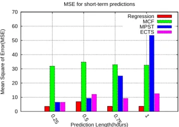
In Fig. 5.1 and Fig. 5.2, we compare the prediction methods for short-term and long-term prediction. In these two experiments, the parameters of MCF and MPST are the best parameters in the experiment, as shown in Fig.5.5, 5.6, 5.7 and 5.8. The difference between short-term and long-term is the prediction length, and the prediction is short-term if it is less than 1 hour. This breakpoint is decided from our data set. The sampling rate of our data set
0 10 20 30 40 50 60 70 0.25 0.5 0.75 1
Mean Square of Error(MSE)
Prediction Length(hours) MSE for short-term predictions
Regression MCF MPST ECTS
Figure 5.1: Prediction results for short-term prediction
0 100 200 300 400 500 1 2 3 4 5 6
Mean Square of Error(MSE)
Prediction Length(hours) MSE for long-term predictions
Regression MCF MPST ECTS
Figure 5.2: Prediction results for long-term prediction
0 20 40 60 80 100 120 140 160
Mean Square of Error(MSE)
Prediction Methods MSE for different prediction methods
Regression MCF MPST Hbrid ECTS
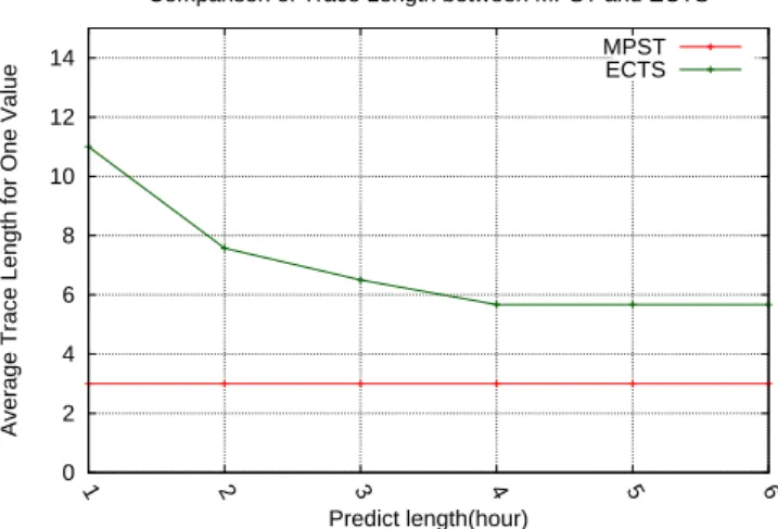
0 2 4 6 8 10 12 14 1 2 3 4 5 6
Average Trace Length for One Value
Predict length(hour)
Comparison of Trace Length between MPST and ECTS MPST ECTS
Figure 5.4: Comparison average trace length of MPST and ECTS
is 1 minute. In the short-term predictions, each is a continuous prediction for the values of 15 minutes after the prediction length. For example, the prediction length of 0.5 hour means to predict the values at tc + 31 tc + 45. As the results show in Fig. 5.1, regression is the best
prediction method, as we mentioned, for short-term predictions. For long-term predictions, each experiment is continuous predictions for the values of 1 hour. Although MPST is not always the most accurate prediction method, it is better than regression, MCF and ECTS on most occasions.
Although the accuracy of MPST is close to that of ECTS, our MPST is better than ECTS on the tracing length. The tracing length is how far we should trace back the time series to predict a value. In Fig. 5.4, we compared the average tracing length of MPST and ECTS. In this experiment, ECTS needs a longer tracing length, and the needed tracing length is not fixed. Therefore our MPST uses less data than ECTS, and the accuracy of MPST is close to that of ECTS.
To summarize the above results, we did an experiment of 6 hours continuous prediction, the results of which are shown in Fig. 5.3. In this experiment, the parameters of the prediction methods are the same as in the above experiments. The hybrid prediction in this experiment is the most accurate prediction method. In this experiment the threshold of hybrid prediction is 1 hour; therefore we use regression when the prediction length is less than 1 hour and MPST when it exceeds 1 hour.
We also carried out the experiment using our clustering-based methods. In Fig. 5.5, 5.6, 5.7 and 5.8, we use different parameters for the clustering-based prediction methods MCF and
0 20 40 60 80 100 2 4 6 8 12
Mean Square of Error(MSE)
period(hour)
MSE for different time series period MCF
Figure 5.5: Different periods for MCF
0 20 40 60 80 100 5 10 15 20 30
Mean Square of Error(MSE)
period(min)
MSE for different time series periods MPST
Figure 5.6: Different periods for MPST
0 10 20 30 40 50 2 3 4 5 6 7 8
Mean Square of Error(MSE)
MPST height MSE for different MPST heights
MPST
0 10 20 30 40 50 0 1 2 3 4 5 6 7 8
Mean Square of Error(MSE)
threshold
MSE for different similarity thresholds MPST
Figure 5.8: Different pattern similarity threshold for MPST
MPST to investigate the effect of the parameters. In MCF, there are only two parameters: k and time series period. The parameter k is for clustering algorithm k-means. The value of k affects the clustering result of both MCF and MPST; therefore we will discuss this issue with MPST. The experiment result for the time series period of MCF is shown in Fig. 5.5. As can be seen, the best time series period for MCF when using our data set is 4 hours.
In Fig. 5.6, we used different time series periods for MPST. Because it predicts the future value using several recent patterns, the period is shorter than in MCF. If the period is 30 minutes and the MPST height is 3, MPST will use the recent data of 1.5 hours to predict the next 30 minutes. In this experiment, we found that 10 minutes is the best time series period for MPST when using our data set. The height of MPST is another important parameter. We mentioned that the prediction result is decided from the recent patterns. The height of MPST affects the maximal patterns we use to make predictions. The effect of MPST heights is shown in Fig. 5.7. The effect is not obvious in this experiment because we used the number of occurrences to make the predictions. The number of occurrences is lower and lower in the lower nodes; therefore the effectiveness is also lower. Thus the MPST height is not so important as period. The last parameter of MPST is the pattern similarity threshold. This is the parameter which decides whether the subsequence is like the pattern in the symbolization process. The value of the pattern similarity threshold means: if the distance between the subsequence and the pattern is lower than the threshold, the subsequence is similar to this pattern. As shown in Fig. 5.8, the effect of the threshold is stepwise. When the threshold is greater than 6, the prediction result is inaccurate. This is because a threshold that is too
0 20 40 60 80 100 120 140 0 0.5 1 1.5 2 2.5 3 3.5 4 4.5 5
Average Trace Length for One Value
Predict length(hour)
Comparison of Trace Length between MPST and ECTS Hybrid
Figure 5.9: Different threshold for Hybrid Prediction
0 2 4 6 8 10 12 14 4 6 8 10 12 14 16 18
Number of Clusters After Pruning
Value of K
Clustering Results with Different Values of K k
Figure 5.10: Effect of K in K-means
big causes MPST to use patterns which are not similar to the subsequence to predict future values.
For the hybrid prediction method, we tried different threshold values. The experiment results are shown in Fig. 5.9, The best threshold is 1 hour, therefore we use 1 hour as the breakpoint of the short-term and long-term predictions. In this experiment, a bigger threshold means using much regression; thus accuracy is low with a big threshold.
We mentioned that the value of k in clustering algorithm K-means is not an important parameter. To prove this, we clustered our data set with different values of k and pruned the clusters. This experiment result is shown in Fig. 5.10. When k is big enough, the number of clusters will no longer grow.
that the regression-based method fits for short-term prediction, clustering-based prediction fits for long-term prediction.
Chapter 6
Future Work
Despite the promising results of this work, there are still many issues to be solved. We only use three prediction methods in this work, but there are many other methods which can fit different conditions. We can use more conditions such as similarity with clusters to switch the prediction methods. Hybrid prediction can combine more prediction methods to perform customization for different data types and parameters.
The clustering-based prediction methods are not complete in some details such as how many states there are in MPST. We will find a method to find the time series period and the states of MPST in the future. Moreover, we have only used K-means as our clustering method. However, there are many other existing clustering methods such as hierarchical clustering which can be used to cluster time series data. We can also use different clustering methods for different types of time series. For example, K-means is weak in terms of solving noises problems and so is not suitable for data with noises. Different data should be processed using different clustering methods.
In this work, our proposed method cannot predict time series with growing values over time. We will add prediction methods which can predict this type of data into the hybrid prediction in the future. However, we need a classification algorithm to classify the type of time series. This is another challenging task.
The threshold of the hybrid prediction method is not perfect. We can design a training process of hybrid prediction to train the threshold which can be dynamic when newer values
Chapter 7
Conclusion
In this paper, we studied the existing time series analysis works, and found that they can-not predict the value of different data types. Therefore we proposed 3 prediction methods: regression-based prediction, clustering-based prediction and hybrid prediction. Regression-based prediction is accurate when the query time is not too far from the current time, while clustering-based predictions are more accurate when the query time is far from the current time. To combine the advantages of the above two methods, we proposed hybrid prediction using a prediction length threshold that decides which method to use. We also did many experiments on many real data sets such as traffic status logs to prove the accuracy of our proposed methods. In the experimental results, we verified the correction of the properties of the regression-based prediction and clustering-based prediction methods. We also proved that our hybrid prediction is more accurate than other prediction methods.
Bibliography
[1] D. J. Bemdt and J. Clifford. Using dynamic time warping to find patterns in time series. In KDD Workshop, pages 229 – 248, 1994.
[2] Chris Chatfield. Time-Series Forecasting. Chapman and Hall/CRC, 2001.
[3] L. Chen and R. T. Ng. On the marriage of lp-norms and edit distance. In VLDB, 2004.
[4] L. Chen, M. T. Ozsu, , and V. Oria. Robust and fast similarity search for moving object trajectories. In SIGMOD, pages 491 – 502, 2005.
[5] Martin Ester, Hans-Peter Kriegel, J¨org Sander, and Xiaowei Xu. A density-based algo-rithm for discovering clusters in large spatial databases with noise. In KDD, 1996.
[6] C.L. Giles, S. Lawrence, and A.C. Tsoi. Noisy time series prediction using recurrent neural networks and grammatical inference. In Machine Learning, 2001.
[7] X. Gu and H. Wang. Online anomaly prediction for robust cluster systems. In ICDE, 2009.
[8] J. Lin, E. Keogh, L. Wei, and S. Lonardi. Experiencing sax: a novel symbolic represen-tation of time series. Data Mining and Knowledge Discovery, 15(2):107–144, 2007.
[9] S. Lloyd. Least squares quantization in pcm. In IEEE Transactions on Information
Theory, 1982.
[10] Amy McGovern, Derek H. Rosendahl, Rodger A. Brown, and Kelvin Droegemeier. Iden-tifying predictive multi-dimensional time sreies motifs: An application to severe weatther prediction. In Data Mining and Knowledge Discovery, 2011.
[11] You min Ha, Sanghyun Park, Sang-Wook Kim, Jung-Im Won, and Jee-Hee Yoon. Rule discovery and matching in stock databases. In IEEE International Computer Software
and Applications Conference, 2008.
[12] F. Morchen, A. Ultsch, and O. Hoos. Extracting interpretable muscle activation patterns with time series knowledge mining. INTERNATIONAL JOURNAL OF KNOWLEDGE
BASED INTELLIGENT ENGINEERING SYSTEMS, 9(3):197, 2005.
[13] Abdullah Mueen and Eamonn keogh. Online discovery and maintenance of time series motifs. In KDD, 2010.
[14] Abdullah Mueen, Eamonn keogh, and Nima Bigdely-Shamlo. Finding time series motifs in disk-resident data. In ICDM, 2009.
[15] Dana Ron, Yoram Singer, and Naftali Tishby. The power of amnesia: Learning proba-bilistic automata with variable memory length. In Machine Leraning, 1996.
[16] Dymitr Ruta, Bogdan Gabrys, and Christiane Lemke. A generic multilevel architecture for time series prediction. In TKDE, 2010.
[17] A. Sant’Anna and N. Wickstrom. Symbolization of time-series: An evaluation of sax, persist, and aca. In Image and Signal Processing (CISP), 2011 4th International Congress
on, volume 4, pages 2223–2228. IEEE, 2011.
[18] Y. Tan, X. Gu, and H. Wang. Adaptive system anomaly prediction for large-scale hosting infrastructures. In PODC, 2010.
[19] R.S. Tsay. Analysis of Financial Time Series. John Wiley&Sons, 2002.
[20] M. Vlachos, G. Kollios, , and D. Gunopulos. Discovering similar multidimensional tra-jectories. In ICDE, pages 673 – 684, 2002.
[21] Michail Vlachos, Philip Yu, and Vittorio Castelli. On periodicity detection and structural periodic similarity. In SDM, 2005.
[22] Peng Wang, Haixun Wang, and Wei Wang. Finding semantics in time series. In SIGMOD, 2011.
[23] Zhengzheng Xing, Jian Pei, and Philip S. Yu. Early classification on time series. In KAIS, 2012.
[24] Pengcheng Xiong, Yun Chi, Shenghuo Zhu, Hyun Jin Moon, Calton Pu, and Hakan Hacıg¨um¨us. Intelligent management of virtualized resources for database systems in cloud environment. In SDM, 2005.
[25] Hang Yuan, Jianhua Liu, Hailin Pu, Jiasong Mao, and Shan Gao. Prediction of chaotic ferroresonance time series based on the dynamic fuzzy neural network. In ECAC, 2012.
[26] F. Zhou, F. Torre, and J.K. Hodgins. Aligned cluster analysis for temporal segmentation of human motion. In Automatic Face & Gesture Recognition, 2008. FG’08. 8th IEEE