Implementation on Electronic Circuits and RTR Pragmatical Adaptive Synchronization: Time-Reversed Uncertain Dynamical Systems' Analysis and Applications

(1)

Volume 2013, Article ID 909721,10pages http://dx.doi.org/10.1155/2013/909721

Research Article

Implementation on Electronic Circuits and RTR Pragmatical

Adaptive Synchronization: Time-Reversed Uncertain Dynamical

Systems’ Analysis and Applications

Shih-Yu Li,

1,2

Cheng-Hsiung Yang,

3

Li-Wei Ko,

1,2

Chin-Teng Lin,

2,4

and Zheng-Ming Ge

5

1_{Department of Biological Science and Technology, National Chiao Tung University, 1001 Ta Hsueh Road, Hsinchu 300, Taiwan} 2_{Brain Research Center, National Chiao Tung University, Hsinchu, Taiwan}

3_{Graduate Institute of Automation and Control, National Taiwan University of Science and Technology, Taipei, Taiwan} 4_{Institute of Electrical Control Engineering, National Chiao Tung University, Hsinchu, Taiwan}

5_{Department of Mechanical Engineering, National Chiao Tung University, Hsinchu, Taiwan}

Correspondence should be addressed to Shih-Yu Li; [email protected] Received 18 October 2012; Accepted 27 January 2013

Academic Editor: Gani Stamov

Copyright © 2013 Shih-Yu Li et al. This is an open access article distributed under the Creative Commons Attribution License, which permits unrestricted use, distribution, and reproduction in any medium, provided the original work is properly cited. We expose the chaotic attractors of time-reversed nonlinear system, further implement its behavior on electronic circuit, and apply the pragmatical asymptotically stability theory to strictly prove that the adaptive synchronization of given master and slave systems with uncertain parameters can be achieved. In this paper, the variety chaotic motions of time-reversed Lorentz system are investigated through Lyapunov exponents, phase portraits, and bifurcation diagrams. For further applying the complex signal in secure communication and file encryption, we construct the circuit to show the similar chaotic signal of time-reversed Lorentz system. In addition, pragmatical asymptotically stability theorem and an assumption of equal probability for ergodic initial conditions (Ge et al., 1999, Ge and Yu, 2000, and Matsushima, 1972) are proposed to strictly prove that adaptive control can be accomplished successfully. The current scheme of adaptive control—by traditional Lyapunov stability theorem and Barbalat lemma, which are used to prove the error vector—approaches zero, as time approaches infinity. However, the core question—why the estimated or given parameters also approach to the uncertain parameters—remains without answer. By the new stability theory, those estimated parameters can be proved approaching the uncertain values strictly, and the simulation results are shown in this paper.

1. Introduction

Nonlinear dynamics, commonly called the chaos theory, changes the scientific way of looking at the dynamics of natural and social systems, which has been intensively studied over the past several decades [1–11]. The phenomenon of chaos has attracted widespread attention amongst math-ematicians, physicists, and engineers and has also been extensively studied in many fields, such as chemical reactions [12, 13], biological systems [14, 15], information processing [16,17], secure communications [18–21], and the rest.

Whilst many researchers analyze complicated, physically motivated configurations, there is also a need to investigate simple equations in a complete different sight view, which

may capture the essence of chaos in a less involved setting, thereby aiding the understanding of essential characteristics. The most well-famous and classical nonlinear chaotic system should be “Lorenz system,” which is an extraordinary three-dimensional nonlinear system originally investigated by the mathematical meteorologist Lorenz [22], who discovered chaos in a simple system of three autonomous ordinary differential equations in order to describe the simplified Rayleigh-Benard problem in 1963. After that, the nonlinear behaviors of Lorentz system are regarded as an important research topic, and plenty of articles are focusing on Lorentz system and its extensive system (which is called family of Lorentz systems or Lorentz-like system) studying [23–

(2)

Although Lorentz-related systems have been made a thorough study, most of the existing articles are studying these kinds of systems via changing the parameters, adding an alternative nonlinear terms (feedback control), or inputting additional signals to the parameter or feedback terms. Besides, there are some articles [27–29] in studying changing time scale to find out if there exist different phenomena in nonlinear systems. The researches in [27–29] are only concentrating on different time scales, and the nonlinear systems differential with respect to negative time are not touched in such articles. As a result, in this paper, we follow the art of Ge and Li [30] to widen a new field of vision in Lorentz system with negative time and express the fruitful dynamics in this time-reversed Lorentz system. The proposing and the thorough understanding of the physical essence for time-reversed chaotic systems are quite beneficial for further studies of dynamically rich chaotic systems. Most importantly, the proposing time-reversed Lorentz system still satisfies the condition𝑎₁₂𝑎₂₁ > 0, which is defined via Liu and Barbosa [31]. On the other hand, for further applying the chaotic signal to secure communication and file encryption, we construct the circuit to show the similar chaotic signal of time-reversed Lorentz system. The same initial conditions and parameters are given for comparison between MATLAB and circuits, which shows high similarity.

Synchronization of chaotic systems is essential in variety of applications, including secure communication, physiology, and nonlinear optics. Accordingly, following the initial work of Pecora and Carroll [32] in synchronization of identi-cal chaotic systems with different initial conditions, many approaches have been proposed for the synchronization of chaotic and hyperchaotic systems. However, most of the methods are used to synchronize only two systems with exactly known structures and parameters, but in practical situations, some or all of the systems’ parameters cannot be exactly known in priori. As a result, more and more applications of chaos synchronization in secure communi-cation have made it much more important to synchronize two different dynamics systems with uncertain parameters in recent years. In this regard, some works on synchronization of two different dynamical systems with uncertain parameters have been performed [33–37]. In current scheme of adaptive synchronization, traditional Lyapunov stability theorem and Barbalat lemma are used to prove that the error vector approaches zero, as time approaches infinity, but the question that why those estimated parameters also approach the uncer-tain values remains without answer. In this paper, pragmatical asymptotically stability theorem and an assumption of equal probability for ergodic initial conditions [38–40] are used to prove strictly that those estimated parameters approach the uncertain values. By the new stability theory, those estimated parameters can be proved approaching the uncertain values strictly, and the simulation results are shown in this paper.

The layout of the rest of the paper is as follows. In

Section 2, classical and time-reversed Lorentz systems are introduced, given complete information of comparison. In

Section 3, pragmatical adaptive synchronization scheme is presented. In Section 4, adaptive RTR synchronization of master and slave systems through pragmatical asymptotically

−10 −20 −10 −20 −30 −15 −5 5 10 15 20 30 20 10 0 0 𝑥2 (𝑡 ) 𝑥1(𝑡) (a) −10 −20 −10 −20 −15 −5 0 5 10 15 20 30 20 10 0 𝑥3 (𝑡 ) 𝑥1(𝑡) (b)

Figure 1: Projections of phase portrait of chaotic classical Lorentz

system with𝑎 = 10, 𝑏 = 8/3, and 𝑐 = 28.

stability is operated, and the well-performed simulation results are provided. InSection 5, conclusions are given.

2. Lorentz System and Time-Reversed

Lorentz System

First of all, let us review the classical Lorentz system [21], which is an extraordinary three-dimensional nonlinear sys-tem proposed by the mathematical meteorologist Lorenz. The well-known equation is shown as follow:

𝑑𝑥₁(𝑡) 𝑑𝑡 = 𝑎 (𝑥2(𝑡) − 𝑥1(𝑡)) , 𝑑𝑥₂(𝑡) 𝑑𝑡 = 𝑐𝑥1(𝑡) − 𝑥1(𝑡) 𝑥3(𝑡) − 𝑥2(𝑡) , 𝑑𝑥₃(𝑡) 𝑑𝑡 = 𝑥1(𝑡) 𝑥2(𝑡) − 𝑏𝑥3(𝑡) . (1)

Given initial condition(𝑥₁₀, 𝑥₂₀, 𝑥₃₀) = (−0.1, 0.2, 0.3) and parameters𝑎 = 10, 𝑏 = 8/3, and 𝑐 = 28, chaos of (1) appears, where the parameters 𝑎 and 𝑐 are satisfying the condition: 𝑎𝑐 > 0. The chaotic behavior of (1) is shown inFigure 1.

Time-reversed Lorentz equations are provided as follows [30]: 𝑑𝑥1(−𝑡) 𝑑 (−𝑡) = 𝑎 (𝑥2(−𝑡) − 𝑥1(−𝑡)) , 𝑑𝑥₂(−𝑡) 𝑑 (−𝑡) = 𝑐𝑥1(−𝑡) − 𝑥1(−𝑡) 𝑥3(−𝑡) − 𝑥2(−𝑡) , 𝑑𝑥₃(−𝑡) 𝑑 (−𝑡) = 𝑥1(−𝑡) 𝑥2(−𝑡) − 𝑏𝑥3(−𝑡) . (2)

It is clear that in the left hand sides of (2), the derivatives are taken with the back time. We will aims to express the

(3)

Table 1: Dynamic behaviors of historical Lorentz system for different signs of parameters.

𝑎 𝑏 𝑐 States − + + Approach to infinite + − + Approach to infinite + + − Periodic − − + Approach to infinite − + − Approach to infinite

− − − Chaos and periodic

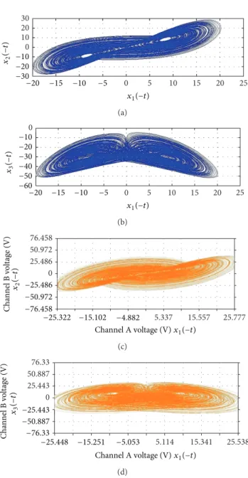
25 20 15 10 30 20 10 0 0 5 −10 −10 −20 −20 −30 −15 −5 𝑥2 (− 𝑡) 𝑥1(−𝑡) (a) 0 25 20 15 10 0 5 −10 −20 −30 −40 −60 −50 −10 −20 −15 −5 𝑥3 (− 𝑡) 𝑥1(−𝑡) (b)

Figure 2: Projections of phase portrait of chaotic historical Lorenz

system with𝑌 in 𝑎 = −10, 𝑏 = −8/3, and 𝑐 = −28.

fruitful nonlinear behaviors of the time-reversed Lorentz system and to comprehend the relation with classical one. The simulation results are arranged inTable 1.

When initial condition (𝑥₁₀, 𝑥₂₀, 𝑥₃₀) = (−0.1, 0.2, 0.3) and parameters𝑎 = −10, 𝑏 = −8/3, and 𝑐 = −28, chaos of the time-reversed Lorentz system appears, where the parameters 𝑎 and 𝑐 are also satisfying the condition: 𝑎𝑐 > 0. The chaotic behavior of (2) is shown inFigure 2.

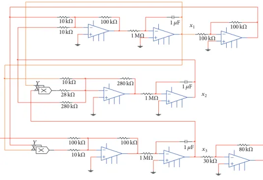
In order to verify the circuit, we have implemented it using an electronics simulation package Multisim (previously called Electronic Workbench, EWB). The electric circuit is presented in Figure 3 to compare with the simulation result in Figure 2. The configuration of electronic circuit for chaotic time-reversed Lorentz system is also given in

Figure 4. The voltage outputs have been normalized to 0.1 V, and the operational amplifiers are considered to be ideal. Hence the default initial conditions are (−0.01 V, 0.02 V, and 0.03 V). Most of the phase diagrams are plotted within the time interval 300–400 s. The time step is 0.001 s. The phase diagrams of the two simulation results given below show that the chaotic signals generated by the electronic circuits can perform high similarity with the original one generated by the ideal simulation tools. Accordingly, the chaotic signals

0 10 20 30 25 20 15 10 0 5 −10 −20 −30 −10 −20 −15 −5 𝑥2 (− 𝑡) 𝑥1(−𝑡) (a) 0 25 20 15 10 0 5 −10 −20 −30 −40 −50 −60 −10 −20 −15 −5 𝑥3 (− 𝑡) 𝑥1(−𝑡) (b) 25.777 15.557 76.458 0 5.337 50.972 25.486 −25.486 −50.972 −76.458 −15.102 −25.322 −4.882 Channel A voltage (V) 𝑥1(−𝑡) Cha nnel B v ol tag e (V) 𝑥2 (− 𝑡) (c) 25.538 15.341 5.114 76.33 50.887 25.443 0 −25.443 −50.887 −76.33 −25.448 −15.251 −5.053 Channel A voltage (V) 𝑥1(−𝑡) Cha nnel B v ol tag e (V) 𝑥3 (− 𝑡) (d)

Figure 3: Projection of phase portraits outputs in electronic circuit for time-reversed Lorenz system.

produced by electronic circuits have high controllability and can be applied to encryption of signals or files.

The different and similar dynamics information between classical and time-reversed Lorentz systems are reported in detail through bifurcation diagrams, Lyapunov expo-nents, and tables. The complete simulation results about the dynamic systems are divided into three parts.

Part 1: changing𝑐, and with 𝑎, 𝑏 fixed, the simulation results are shown inFigure 5.

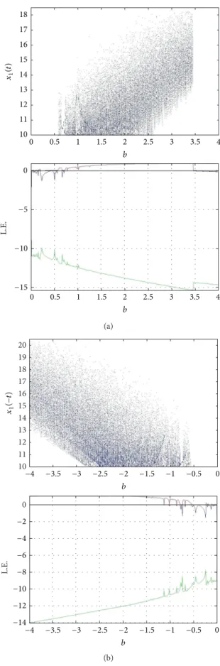
Part 2: changing𝑏, and with 𝑎, 𝑐 fixed, the simulation results are shown inFigure 6.

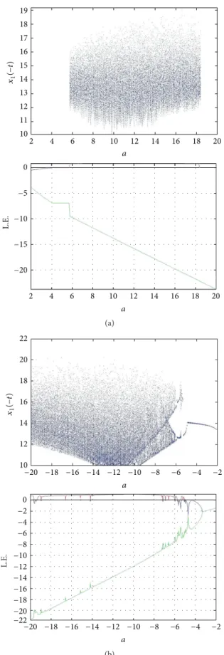
Part 3: changing𝑎, and with 𝑏, 𝑐 fixed, the simulation results are shown inFigure 7.

(4)

10 kΩ 10 kΩ 10 kΩ 10 kΩ 100 kΩ 100 kΩ 100 kΩ 100 kΩ 100 kΩ 1 MΩ 1 MΩ 1 MΩ 28 kΩ 30 kΩ 1 𝜇F 1 𝜇F 1 𝜇F + ₊ + + + + + + − ₋ − − − − − − 𝑋𝑌 𝑋𝑌 280 kΩ 280 kΩ 80 kΩ 𝑥1 𝑥2 𝑥3

Figure 4: The electronic circuit of chaotic time-reversed Lorenz system.

3. Pragmatical Adaptive

Synchronization Scheme

3.1. Adaptive Synchronization Scheme. There are two identical

nonlinear dynamical systems, and the master system controls the slave system. The master system is given by

̇𝑥 = 𝐴𝑥 + 𝑓 (𝑥, 𝐵) , (3) where 𝑥 = [𝑥₁, 𝑥₂, . . . , 𝑥_𝑛]𝑇 ∈ 𝑅𝑛 denotes a state vector, 𝐴 is an 𝑛 × 𝑛 uncertain constant coefficient matrix, 𝑓 is a nonlinear vector function, and 𝐵 is a vector of uncertain constant coefficients in𝑓.

The slave system is given by

̇𝑦 = ̂𝐴𝑦 + 𝑓 (𝑦, ̂𝐵) + 𝑢 (𝑡) , (4) where𝑦 = [𝑦₁, 𝑦₂, . . . , 𝑦_𝑛]𝑇 ∈ 𝑅𝑛denotes a state vector, ̂𝐴 is an𝑛×𝑛 estimated coefficient matrix, ̂𝐵 is a vector of estimated coefficients in𝑓, and 𝑢(𝑡) = [𝑢₁(𝑡), 𝑢₂(𝑡), . . . , 𝑢_𝑛(𝑡)]𝑇∈ 𝑅𝑛is a control input vector.

Our goal is to design a controller𝑢(𝑡), so that the state vector of the chaotic system (3) asymptotically approaches the state vector of the master system (4).

The chaos synchronization can be accomplished in the sense that the limit of the error vector𝑒(𝑡) = [𝑒₁, 𝑒₂, . . . , 𝑒_𝑛]𝑇 approaches zero as follows:

lim 𝑡 → ∞𝑒 = 0, (5) where 𝑒 = 𝑥 − 𝑦. (6) From (6) we have ̇𝑒 = ̇𝑥 − ̇𝑦, (7) ̇𝑒 = 𝐴𝑥 − ̂𝐴𝑦 + 𝑓 (𝑥, 𝐵) − 𝑓 (𝑦, ̂𝐵) − 𝑢 (𝑡) . (8) A Lyapunov function 𝑉(𝑒, ̃𝐴_𝑐, ̃𝐵_𝑐) is chosen as a positive definite function

𝑉 (𝑒, ̃𝐴, ̃𝐵) = 1₂𝑒𝑇𝑒 +1₂𝐴̃𝑇𝐴 +̃ 1₂̃𝐵𝑇̃𝐵, (9) where ̃𝐴 = 𝐴 − ̂𝐴, ̃𝐵 = 𝐵 − ̂𝐵, and ̃𝐴_𝑐and ̃𝐵_𝑐are two column matrices whose elements are all the elements of matrix ̂𝐴 and of matrix ̂𝐵, respectively.

Its derivative along any solution of the differential equa-tion system consisting of (8) and update parameter differen-tial equations for ̃𝐴_𝑐and ̃𝐵_𝑐is

̇𝑉 (𝑒, ̃𝐴𝑐, ̃𝐵𝑐) = 𝑒𝑡[𝐴𝑥 − ̂𝐴𝑦 + 𝐵𝑓 (𝑥) − ̂𝐵𝑓 (𝑦) − 𝑢 (𝑡)] + ̃𝐴_𝑐 ̇̃𝐴_𝑐+ ̃𝐵_𝑐 ̇̃𝐵_𝑐,

(10)

where 𝑢(𝑡), ̇̃𝐴_𝑐, and ̇̃𝐵_𝑐 are chosen so that ̇𝑉 = 𝑒𝑇𝐶𝑒, 𝐶 is a diagonal negative definite matrix, and ̇𝑉 is a negative semidefinite function of𝑒 and parameter differences ̃𝐴_𝑐and ̃𝐵𝑐. In current scheme of adaptive control of chaotic motion [33–37], traditional Lyapunov stability theorem and Barbalat lemma are used to prove that the error vector approaches zero, as time approaches infinity. But the question, why the estimated or given parameters also approach to the uncertain or goal parameters, remains without answer. By pragmatical asymptotical stability theorem, the question can be answered strictly.

(5)

35 30 25 20 15 10 20 25 30 35 40 45 50 55 60 65 70 𝐶 20 25 30 35 40 45 50 55 60 65 70 𝐶 0 −2 −4 −6 −8 −10 −12 −14 L.E. 𝑥1 (𝑡 ) (a) 35 30 25 20 10 15 −70 −65 −60 −55 −50 −45 −40 −35 −30 −25 −20 𝐶 𝑥1 (− 𝑡) 0 L.E. −2 −4 −6 −8 −10 −12 −70 −65 −60 −55 −50 −45 −40 −35 −30 −25 −20 𝐶 (b)

Figure 5: (a) Bifurcation diagram and Lyapunov exponents of

chaotic classical Lorentz system with 𝑏 = 8/3 and 𝑎 = 10.

(b) Bifurcation diagram and Lyapunov exponents of chaotic

time-reversed Lorentz system with𝑏 = −8/3 and 𝑎 = −10. The tables given

previously show the different dynamic characters between classical and time-reversed Lorentz.

𝑏 L.E. 18 17 16 15 14 13 12 11 10 0 0.5 1 1.5 2 2.5 3 3.5 4 𝑏 0 0.5 1 1.5 2 2.5 3 3.5 4 0 −5 −10 −15 𝑥1 (𝑡 ) (a) 15 14 13 12 10 11 16 17 18 19 20 −4 −3.5 −3 −2.5 −2 −1.5 −1 −0.5 0 𝑏 𝑥1 (− 𝑡) L.E. 0 −2 −4 −6 −8 −10 −12 −14 −4 −3.5 −3 −2.5 −2 −1.5 −1 −0.5 0 𝑏 (b)

chaotic classical Lorentz system with 𝑐 = 28 and 𝑎 = 10.

time-reversed Lorentz system with𝑐 = −28 and 𝑎 = −10. The tables

given previously show the different dynamic characters between classical and time-reversed Lorentz systems with different ranges of

(6)

15 14 13 12 10 11 4 6 8 10 12 14 16 18 20 16 17 18 19 2 𝑎 𝑥1 (− 𝑡) 0 L.E. −5 −10 −15 −20 4 6 8 10 12 14 16 18 20 2 𝑎 (a) 22 20 16 18 14 12 10 0 −2 −4 −6 −8 −10 −12 −14 −16 −18 −20 −22 −2 −4 −6 −8 −10 −12 −14 −16 −18 −20 L.E. 𝑎 −2 −4 −6 −8 −10 −12 −14 −16 −18 −20 𝑎 𝑥1 (− 𝑡) (b)

chaotic classical Lorentz system with 𝑏 = 8/3 and 𝑐 = 28.

time-reversed Lorentz system with𝑏 = −8/3 and 𝑐 = −28. The tables

given previously show the different dynamic characters between classical and time-reversed Lorentz systems with different ranges of

parameter𝑎.

3.2. Pragmatical Asymptotical Stability Theory. The stability

for many problems in real dynamical systems is actual asymptotical stability, although it may not be mathematical asymptotical stability. The mathematical asymptotical stabil-ity demands that trajectories from all initial states in the neighborhood of zero solution must approach the origin as 𝑡 → ∞. If there are only a small part or even a few of the initial states from which the trajectories do not approach the origin as 𝑡 → ∞, the zero solution is not mathematically asymptotically stable. However, when the probability of occurrence of an event is zero, it means that the event does not occur actually. If the probability of occurrence of the event that the trajectories from the initial states are that they do not approach zero when𝑡 → ∞ is zero, the stability of zero solution is actual asymptotical stability, though it is not mathematical asymptotical stability. In order to analyze the asymptotical stability of the equilibrium point of such systems, the pragmatical asymptotical stability theorem is used.

Let 𝑋 and 𝑌 be two manifolds of dimensions 𝑚 and 𝑛 (𝑚 < 𝑛), respectively, and let 𝜑 be a differentiable map from 𝑋 to 𝑌, then 𝜑(𝑋) is subset of Lebesque measure 0 of 𝑌 [40]. For an autonomous system

𝑑𝑥

𝑑𝑡 = 𝑓 (𝑥1, . . . , 𝑥𝑛) , (11) where𝑥 = [𝑥₁, . . . , 𝑥_𝑛]𝑇is a state vector, the function𝑓 = [𝑓₁, . . . , 𝑓_𝑛]𝑇is defined on𝐷 ⊂ 𝑅𝑛and‖𝑥‖ ≤ 𝐻 > 0. Let 𝑥 = 0 be an equilibrium point for the system (11). Then

𝑓 (0) = 0. (12)

Definition 1. The equilibrium point for the system (11) is

pragmatically asymptotically stable provided that with initial points on𝐶 which is a subset of Lebesque measure 0 of 𝐷, the behaviors of the corresponding trajectories cannot be deter-mined, while with initial points on𝐷 − 𝐶, the corresponding trajectories behave as that agree with traditional asymptotical stability [33–37].

Theorem 2. Let 𝑉 = [𝑥₁, . . . , 𝑥_𝑛]𝑇:𝐷 → 𝑅₊ be positive

definite and analytic on D, such that the derivative of𝑉

through (11), ̇𝑉, is negative semidefinite. Let 𝑋 be the

m-manifold consisted of point set for which∀𝑥 ̸= 0, ̇𝑉(𝑥) = 0, and

𝐷 is a n-manifold. If 𝑚 + 1 < 𝑛, then the equilibrium point of

the system is pragmatically asymptotically stable.

Proof. Since every point of𝑋 can be passed by a trajectory

of (11), which is one-dimensional, the collection of these trajectories,𝐴, is a (𝑚 + 1)-manifold [38,39].

If𝑚 + 1 < 𝑛, then the collection 𝐶 is a subset of Lebesque measure 0 of𝐷. By the previous definition, the equilibrium point of the system is pragmatically asymptotically stable.

If an initial point is ergodicity chosen in𝐷, the probability of that the initial point falls on the collection 𝐶 is zero. Here, equal probability is assumed for every point chosen as an initial point in the neighborhood of the equilibrium point. Hence, the event that the initial point is chosen from collection𝐶 does not occur actually. Therefore, under

(7)

the equal probability assumption, pragmatical asymptotical stability becomes actual asymptotical stability. When the initial point falls on𝐷 − 𝐶, ̇𝑉(𝑥) < 0, the corresponding trajectories behave as that agree with traditional asymptotical stability because by the existence and uniqueness of the solution of initial-value problem, these trajectories never meet𝐶.

In (9) 𝑉 is a positive definite function of 𝑛 variables, that is,𝑝 error state variables and 𝑛 − 𝑝 = 𝑚 differences between unknown and estimated parameters, while ̇𝑉 = 𝑒𝑇_{𝐶𝑒 is a negative semidefinite function of 𝑛 variables. Since} the number of error state variables is always more than one, 𝑝 > 1, 𝑚 + 1 < 𝑛 is always satisfied, and by pragmatical asymptotical stability theorem we have

lim

𝑡 → ∞𝑒 = 0 (13)

and the estimated parameters approach the uncertain param-eters. The pragmatical adaptive control theorem is obtained. Therefore, the equilibrium point of the system is prag-matically asymptotically stable. Under the equal probability assumption, it is actually asymptotically stable for both error state variables and parameter variables.

4. Pragmatical Adaptive RTR

Synchronization of Master Lorentz System

and Slave Time-Reversed Lorentz System

In this section, adaptive regular and time-reversed (RTR) synchronization from time-reversed Lorentz system (with respect to negative time) to regular Lorentz system (with respect to positive time) is proposed. The time-reversed Lorentz system is considered as slave system, and the regular Lorenz system is regarded as master system. These two equations are shown as follows.

Master system—contemporary Lorenz system: 𝑑𝑥₁(𝑡) 𝑑𝑡 = 𝑎 (𝑥2(𝑡) − 𝑥1(𝑡)) , 𝑑𝑥₂(𝑡) 𝑑𝑡 = 𝑐𝑥1(𝑡) − 𝑥1(𝑡) 𝑥3(𝑡) − 𝑥2(𝑡) , 𝑑𝑥₃(𝑡) 𝑑𝑡 = 𝑥1(𝑡) 𝑥2(𝑡) − 𝑏𝑥3(𝑡) . (14)

Slave system—historical Lorenz system: 𝑑𝑦₁(−𝑡) 𝑑 (−𝑡) = −̂𝑎 (𝑦2(−𝑡) − 𝑦1(−𝑡)) + 𝑢1, 𝑑𝑦₂(−𝑡) 𝑑 (−𝑡) = − (̂𝑐𝑦1(−𝑡) − 𝑦1(−𝑡) 𝑦3(−𝑡) − 𝑦2(−𝑡)) + 𝑢2, 𝑑𝑦₃(−𝑡) 𝑑 (−𝑡) = − (𝑦1(−𝑡) 𝑦2(−𝑡) − ̂𝑏𝑦3(−𝑡)) + 𝑢3, (15) where𝑥_𝑖(𝑡) stands for states variables of the master system, and𝑦_𝑖(−𝑡) stands for the slave system, respectively. Parame-ters,𝑎, 𝑏, and 𝑐 are uncertain parameters of master system. ̂𝑎,

̂𝑏, and̂𝑐are estimated parameters. 𝑢₁,𝑢₂, and𝑢₃are nonlinear controller to synchronize the slave Lorenz system to master one; that is,

lim

𝑡 → ∞𝑒 = 0, (16)

where the error vector𝑒 = [𝑒₁(𝑡) 𝑒₂(𝑡) 𝑒₃(𝑡)] and 𝑒₁(𝑡) = 𝑥₁(𝑡) − 𝑦₁(−𝑡) , 𝑒₂(𝑡) = 𝑥₂(𝑡) − 𝑦₂(−𝑡) , 𝑒₃(𝑡) = 𝑥₃(𝑡) − 𝑦₃(−𝑡) .

(17)

From (17), we have the following error dynamics: 𝑑𝑒₁(𝑡) 𝑑𝑡 = 𝑑𝑥₁(𝑡) 𝑑𝑡 − 𝑑𝑦₁(−𝑡) 𝑑𝑡 = 𝑑𝑥₁(𝑡) 𝑑𝑡 + 𝑑𝑦₁(−𝑡) 𝑑 (−𝑡) , 𝑑𝑒₂(𝑡) 𝑑𝑡 = 𝑑𝑥₂(𝑡) 𝑑𝑡 − 𝑑𝑦₂(−𝑡) 𝑑𝑡 = 𝑑𝑥₂(𝑡) 𝑑𝑡 + 𝑑𝑦₂(−𝑡) 𝑑 (−𝑡) , 𝑑𝑒3(𝑡) 𝑑𝑡 = 𝑑𝑥3(𝑡) 𝑑𝑡 − 𝑑𝑦₃(−𝑡) 𝑑𝑡 = 𝑑𝑥3(𝑡) 𝑑𝑡 + 𝑑𝑦₃(−𝑡) 𝑑 (−𝑡) , ̇𝑒 1= 𝑎 (𝑥2− 𝑥1) + (−̂𝑎 (𝑦2− 𝑦1) + 𝑢1) , ̇𝑒 2= 𝑐𝑥1− 𝑥1𝑥3− 𝑥2+ (− (̂𝑐𝑦1− 𝑦1𝑦3− 𝑦2) + 𝑢2) , ̇𝑒 3= 𝑥1𝑥2− 𝑏𝑥3+ (− (𝑦1𝑦2− ̂𝑏𝑦3) + 𝑢3) . (18)

The two systems will be synchronized for any initial con-dition by appropriate controllers and update laws for those estimated parameters. As a result, the following controllers and update laws are designed by pragmatical asymptotical stability theorem as follows.

Choosing Lyapunov function as 𝑉 =1

2(𝑒21+ 𝑒22+ 𝑒23+ ̃𝑎2+ ̃𝑏 2

+ ̃𝑐2) , (19) wherẽ𝑎 = 𝑎 − ̂𝑎, ̃𝑏 = 𝑏 − ̂𝑏, and ̃𝑐 = 𝑐 − ̂𝑐.

Its time derivative is

̇𝑉 = 𝑒₁ ̇𝑒1+ 𝑒2 2̇𝑒 + 𝑒3 ̇𝑒3+ ̃𝑎 ̇̃𝑎 + ̃𝑏 ̇̃𝑏 + ̃𝑐 ̇̃𝑐 = 𝑒₁(𝑎 (𝑥₂− 𝑥₁) + (−̂𝑎 (𝑦₂− 𝑦₁) + 𝑢₁)) + 𝑒₂(𝑐𝑥₁− 𝑥₁𝑥₃− 𝑥₂+ (− (̂𝑐𝑦₁− 𝑦₁𝑦₃− 𝑦₂) + 𝑢₂)) + 𝑒₃(𝑥₁𝑥₂− 𝑏𝑥₃+ (− (𝑦₁𝑦₂− ̂𝑏𝑦₃) + 𝑢₃)) + ̇̃𝑎 (𝑎 − ̂𝑎) + ̇̃𝑏 (𝑏 − ̂𝑏) + ̇̃𝑐 (𝑐 − ̂𝑐) . (20) We choose the update laws for those uncertain parame-ters as

̇̃𝑎 = − ̇̂𝑎 = − (𝑥₂− 𝑥₁) 𝑒₁+ ̃𝑎𝑒₁, ̇̃𝑐 = − ̇̂𝑐 = − (𝑥₁) 𝑒₂+ ̃𝑐𝑒₂, ̇̃𝑏 = − ̇̂𝑏 = (𝑥3) 𝑒3+ ̃𝑏𝑒3.

(8)

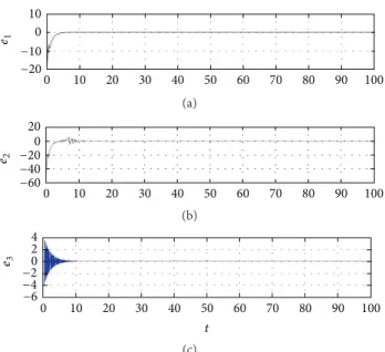
10 0 10 20 30 40 50 60 70 80 90 100 0 −10 −20 𝑒1 (a) 10 20 30 40 50 60 70 80 90 100 0 20 0 −60 −20 −40 𝑒2 (b) 10 20 30 40 50 60 70 80 90 100 0 4 2 0 −6 −2 −4 𝑒3 𝑡 (c)

Figure 8: Time histories of errors for master and slave chaotic Lorentz systems. 10 20 30 40 50 60 70 80 90 100 0 20 10 0 −10 ̃𝑎 (a) 10 20 30 40 50 60 70 80 90 100 0 10 0 −10 −20 ̃𝑏 (b) 10 20 30 40 50 60 70 80 90 100 0 60 40 0 20 −20 ̃𝑐 𝑡 (c)

Figure 9: Time histories of parametric errors for master and slave chaotic Lorentz systems.

Through (21) and (22), the appropriate controllers can be designed as 𝑢₁= −̂𝑎 (𝑥₂− 𝑥₁− 𝑦₂+ 𝑦₁) − ̃𝑎2_{− 𝑒} 1, 𝑢₂= −̂𝑐 (𝑥₁− 𝑦₁) + 𝑥₁𝑥₃+ 𝑥₂+ 𝑦₁𝑦₃+ 𝑦₂− ̃𝑐2− 𝑒₂, 𝑢₃= ̂𝑏 (𝑥₃− 𝑦₃) − 𝑥₁𝑥₂− 𝑦₁𝑦₂− ̃𝑏2− 𝑒₃. (22) We obtain ̇𝑉 = −𝑒2 1− 𝑒22− 𝑒23< 0, (23) 40 20 0 −20 −100 −80 −60 −40 −20 0 20 40 60 80 100 𝑡 𝑥1(𝑡) 𝑦1(−𝑡) (a) 100 50 0 −100 −100 −80 −60 −40 −20 0 20 40 60 80 100 𝑡 𝑥2(𝑡) 𝑦2(−𝑡) (b) 50 40 30 20 10 0 −100 −80 −60 −40 −20 0 20 40 60 80 100 𝑡 𝑥3(𝑡) 𝑦3(−𝑡) (c)

Figure 10: Time histories of states of master and slave chaotic Lorenz systems. 𝑥3 (𝑡 ), 𝑦3 (− 𝑡) 𝑥1(𝑡), 𝑦₁(−𝑡) 𝑥2(𝑡), 𝑦2(− 𝑡) 50 40 30 20 10 0 −20 −15 −10 −5 0 5 10 15 _{20 25 30} −40−20 0 2040 60 𝑥(𝑡) 𝑦(−𝑡)

Figure 11: Phase portraits of synchronization of master and slave chaotic Lorenz systems.

which is negative semidefinite function of𝑒₁, 𝑒₂, 𝑒₃,̂𝑎, ̂𝑏, and̂𝑐. The Lyapunov asymptotical stability theorem is not satisfied. We cannot obtain that common origin of error dynamics (18) and parameter dynamics (21) is asymptotically stable. By pragmatical asymptotically stability theorem,𝐷 is a 6-manifold,𝑛 = 6, and the number of error state variables

(9)

𝑝 = 3. When 𝑒₁ = 𝑒₂ = 𝑒₃ = 0 and ̂𝑎, ̂𝑏, and ̂𝑐 take arbitrary values, ̇𝑉 = 0, 𝑋 is of 3 dimensions, 𝑚 = 𝑛 − 𝑝 = 6 − 3 = 3, and 𝑚 + 1 < 𝑛 is satisfied. According to the pragmatical asymptotically stability theorem, error vector𝑒 approaches zero, and the estimated parameters also approach the uncertain parameters. The equilibrium point is pragmatically asymptotically stable. Under the assumption of equal probability, it is actually asymptotically stable. The simulation results are shown in Figures8,9,10, and11.

5. Conclusions

In this paper, three main contributions are proposed. The first one is exposing the complete information of time-reversed nonlinear system, which providing the range of parameters in detail for researchers to follow and reference; the second one is to realize the chaotic behavior of the time-reversed nonlinear system on electronic circuit, which shows the high corrections between the results by MATLAB and electronic circuits; the third one is to solve the existing problem in non-linear science, applying the pragmatical asymptotically stabil-ity theory to strictly prove that the adaptive synchronization of given master and slave systems with uncertain parameters can be achieved. This paper gives a complete novel sight view to investigate the chaotic attractors and provides a strict mathematical proof to achieve the adaptive synchronization exactly, and for more practical, the chaotic signal generated via electronic circuits can be applied to the communications security, file encryption, biosignal simulation, and so forth.

Acknowledgments

This work was supported in part by the UST-UCSD Inter-national Center of Excellence in Advanced Bioengineering sponsored by the Taiwan National Science Council I-RiCE Program under Grant no. NSC-101-2911-I-009-101. This work was also supported in part by the Aiming for the Top Uni-versity Plan of National Chiao Tung UniUni-versity, the Ministry of Education, Taiwan, under Contract 101W963, supported in part by the Army Research Laboratory, and was accomplished under Cooperative Agreement no. W911NF-10-2-0022.

References

[1] M. S. H. Chowdhury, I. Hashim, S. Momani, and M. M. Rahman, “Application of multistage homotopy perturbation method to the chaotic genesio system,” Abstract and Applied

Analysis, vol. 2012, Article ID 974293, 10 pages, 2012.

[2] H. Luo, “Global attractor of atmospheric circulation equations with humidity effect,” Abstract and Applied Analysis, vol. 2012, Article ID 172956, 15 pages, 2012.

[3] S. Y. Li and Z. M. Ge, “Generating tri-chaos attractors with three positive Lyapunov exponents in new four order system via linear coupling,” Nonlinear Dynamics, vol. 69, no. 3, pp. 805–816, 2012.

[4] C. H. Yang, T. W. Chen, S. Y. Li, C. M. Chang, and Z. M. Ge, “Chaos generalized synchronization of an inertial tachometer with new Mathieu-Van der Pol systems as functional system by GYC partial region stability theory,” Communications in

Nonlinear Science and Numerical Simulation, vol. 17, no. 3, pp.

1355–1371, 2012.

[5] S. Y. Li, C. H. Yang, S. A. Chen, L. W. Ko, and C. T. Lin, “Fuzzy adaptive synchronization of time-reversed chaotic systems via a new adaptive control strategy,” Information Sciences, vol. 222, no. 10, pp. 486–500, 2013.

[6] R. Wu and X. Li, “Hopf bifurcation analysis and anticontrol of Hopf circles of the R¨ossler-like system,” Abstract and Applied

Analysis, vol. 2012, Article ID 341870, p. 16, 2012.

[7] A. Freihat and S. Momani, “Adaptation of differential transform method for the numeric-analytic solution of fractional-order R¨ossler chaotic and hyperchaotic systems,” Abstract and Applied

Analysis, vol. 2012, Article ID 934219, 13 pages, 2012.

[8] Z. M. Ge and S. Y. Li, “Chaos generalized synchronization of new Mathieu-Van der Pol systems with new Duffing-Van der Pol systems as functional system by GYC partial region stability theory,” Applied Mathematical Modelling, vol. 35, no. 11, pp. 5245–5264, 2011.

[9] Z. M. Ge and S. Y. Li, “Chaos control of new Mathieu-Van der Pol systems with new Mathieu-Duffing systems as functional system by GYC partial region stability theory,” Nonlinear

Analysis, Theory, Methods and Applications, vol. 71, no. 9, pp.

4047–4059, 2009.

[10] C. Yin, S. M. Zhong, and W. F. Chen, “Design of sliding mode controller for a class of fractional-order chaotic systems,”

Com-munications in Nonlinear Science and Numerical Simulation, vol.

17, no. 1, pp. 356–366, 2012.

[11] J. Zhao, “Adaptive Q-S synchronization between coupled chaotic systems with stochastic perturbation and delay,” Applied

Mathematical Modelling, vol. 36, no. 7, pp. 3312–3319, 2012.

[12] M. Villegas, F. Augustin, A. Gilg, A. Hmaidi, and U. Wever, “Application of the polynomial chaos expansion to the simula-tion of chemical reactors with uncertainties,” Mathematics and

Computers in Simulation, vol. 82, no. 5, pp. 805–817, 2012.

[13] M. F. P´erez-Polo and M. P´erez-Molina, “Saddle-focus bifurca-tion and chaotic behavior of a continuous stirred tank reactor using PI control,” Chemical Engineering Science, vol. 74, no. 28, pp. 79–92, 2012.

[14] H. Baek, “The dynamics of a predator-prey system with state-dependent feedback control,” Abstract and Applied Analysis, vol. 2012, Article ID 101386, 17 pages, 2012.

[15] B. I. Camara and H. Mokrani, “Analysis of wave solutions of an adhenovirus-tumor cell system,” Abstract and Applied Analysis, vol. 2012, Article ID 590326, 13 pages, 2012.

[16] X. Yuan and H. B. Hwarng, “Managing a service system with social interactions: stability and chaos,” Computers & Industrial

Engineering, vol. 63, no. 4, pp. 1178–1188, 2012.

[17] T. Wang, N. Jia, and K. Wang, “A novel GCM chaotic neu-ral network for information processing,” Communications in

Nonlinear Science and Numerical Simulation, vol. 17, no. 12, pp.

4846–4855, 2012.

[18] J. Machicao, A. G. Marco, and O. M. Bruno, “Chaotic encryption method based on life-like cellular automata,” Expert Systems

with Applications, vol. 39, no. 16, pp. 12626–12635, 2012.

[19] M. M. Juan, L. M. G. Rafael, A. L. Ricardo, and A. I. Carlos, “A chaotic system in synchronization and secure communi-cations,” Communications in Nonlinear Science and Numerical

Simulation, vol. 17, no. 4, pp. 1706–1713, 2012.

[20] Y. Y. Hou, H. C. Chen, J. F. Chang, J. J. Yan, and T. L. Liao, “Design and implementation of the Sprott chaotic secure digital communication systems,” Applied Mathematics and

(10)

[21] C.-J. Cheng, “Robust synchronization of uncertain unified chaotic systems subject to noise and its application to secure communication,” Applied Mathematics and Computation, vol. 219, no. 5, pp. 2698–2712, 2012.

[22] E. N. Lorenz, “Deterministic non-periodic flows,” Journal of the

Atmospheric Science, vol. 20, no. 2, pp. 130–141, 1963.

[23] S. Li, Y. M. Li, B. Liu, and T. Murray, “Model-free control of Lorenz chaos using an approximate optimal control strategy,”

Communications in Nonlinear Science and Numerical Simula-tion, vol. 17, no. 12, pp. 4891–4900, 2012.

[24] D. Cafagna and G. Grassi, “On the simplest fractional-order memristor-based chaotic system,” Nonlinear Dynamics, vol. 70, no. 2, pp. 1185–1197, 2012.

[25] Q. Bi and Z. Zhang, “Bursting phenomena as well as the bifurcation mechanism in controlled Lorenz oscillator with two time scales,” Physics Letters A, vol. 375, no. 8, pp. 1183–1190, 2011.

[26] F. ¨Ozkaynak and A. B. ¨Ozer, “A method for designing strong

S-Boxes based on chaotic Lorenz system,” Physics Letters A, vol. 374, no. 36, pp. 3733–3738, 2010.

[27] A. Vanˇeˇcek and S. ˇCelikovsk´y, Control Systems: From Linear

Analysis to Synthesis of Chaos, Prentice-Hall, London, UK, 1996.

[28] A. El-Gohary and F. Bukhari, “Optimal control of Lorenz system during different time intervals,” Applied Mathematics

and Computation, vol. 144, no. 2-3, pp. 337–351, 2003.

[29] Z. M. Ge and C. C. Chen, “Phase synchronization of coupled chaotic multiple time scales systems,” Chaos, Solitons & Fractals, vol. 20, no. 3, pp. 639–647, 2004.

[30] Z. M. Ge and S. Y. Li, “Yang and Yin parameters in the Lorenz system,” Nonlinear Dynamics, vol. 62, no. 1-2, pp. 105–117, 2010. [31] Y. Liu and L. C. Barbosa, “Periodic locking in coupled Lorenz

systems,” Physics Letters A, vol. 197, no. 1, pp. 13–18, 1995. [32] L. M. Pecora and T. L. Carroll, “Synchronization in chaotic

systems,” Physical Review Letters, vol. 64, no. 8, pp. 821–824, 1990.

[33] K. Salahshoor, M. H. Hajisalehi, and M. H. Sefat, “Nonlinear

model identification and adaptive control of CO₂sequestration

process in saline aquifers using artificial neural networks,”

Applied Soft Computing, vol. 12, no. 11, pp. 3379–3389, 2012.

[34] B. Bhushan and M. Singh, “Adaptive control of DC motor using bacterial foraging algorithm,” Applied Soft Computing, vol. 11, no. 8, pp. 4913–4920, 2011.

[35] R. Ketata, Y. Rezgui, and N. Derbel, “Stability and robustness of fuzzy adaptive control of nonlinear systems,” Applied Soft

Computing Journal, vol. 11, no. 1, pp. 166–178, 2011.

[36] O. Cerman and P. Husek, “Adaptive fuzzy sliding mode control for electro-hydraulic servo mechanism,” Expert Systems with

Applications, vol. 39, no. 11, pp. 10269–10277, 2012.

[37] H. Khayyam, S. Nahavandi, and S. Davis, “Adaptive cruise control look-ahead system for energy management of vehicles,”

Expert Systems with Applications, vol. 39, no. 3, pp. 3874–3885,

2012.

[38] Z. M. Ge, J. K. Yu, and Y. T. Chen, “Pragmatical asymptotical stability theorem with application to satellite system,” Japanese

Journal of Applied Physics,, vol. 38, no. 10, pp. 6178–6179, 1999.

[39] Z. M. Ge and J. K. Yu, “Pragmatical asymptotical stability theorems on partial region and for partial variables with applications to gyroscopic systems,” Journal of Mechanics, vol. 16, no. 4, pp. 179–187, 2000.

(11)