Fully Localized Energy-efficient Multicast in
Large-Scale Wireless Ad Hoc Networks
Tse-Han Huang
Department of Computer Science and Information Engineering
National Taiwan University Email:[email protected]
Ai-Chun Pang
Department of Computer Science and Information Engineering
National Taiwan University Email:[email protected]
Shuo-Cheng Hu
Department of Information Management Shih Hsin University
Email:[email protected]
Wei-Hui Chen
Department of Computer Science and Information Engineering
National Taiwan University Email:[email protected]
Abstract—Most of the proposed distributed
energy-efficient multicasting algorithms are using the local search technology to refine a multicast tree iteratively. They use MST or SPT as the initial solution and improve the total power consumption by switching some tree nodes from their respective parent nodes to new corresponding parent nodes. These algorithms are not scalable because the re-finement operations require heavy message exchange flows. In this paper, we propose the algorithm Localized Energy-efficient Multicast with Grouping (LEMG) features doing local search in a fully localized fashion. The mechanism Grouping exploits a novel idea to evaluate the power consumption cost of every node and limit the message passing within a adjustable constant hop. Our simulation shows LEMG is energy-efficient comparable to DMEM, and the refinement can be done in only limited hops of message passing regardless of the network size and the number of destinations.
Index Terms—Energy efficiency, routing protocols,
wire-less ad hoc network, localized algorithm
I. INTRODUCTION
With the popularity of wireless network, ad hoc network is getting more and more attractive due to their potential applications. Without infrastructure, wireless ad hoc networks are formed by wireless devices in a self-organized and decentralized man-ner. It is flexible and can be deployed easily in any environment. A node in these networks is equipped with an antenna powered by batteries. When the
battery of a node is depleted, it may lead to network disconnection. In order to prolong the network life-time, the energy-aware routing of ad hoc wireless networks has received significant attention.
In the survey [7], there are two main metrics for energy-aware multicast/broadcast routing. Both the two direction receive much attention. For one is energy-efficient routing [18] [2] [3] [11] [10] [12] [6] [16] [5] [13] which wants to minimizing the total power consumption of all nodes in the multicast/broadcast session, the other is maximum lifetime routing [4] [15] [14] [8] which target to maximize the operation time until the battery de-pletion of the first node in the multicast/broadcast session. Some of existing solutions are centralized which may lead to extreme communication over-head for ad hoc network. The others are in a distributed manner; however, knowledge of whole network energy saving information is indispensable to make decision. The amount of messages increases dramatically with the network size. Accordingly, It may cause unacceptable execution time in large-scale networks. Hence, an ideal algorithm or proto-col for ad hoc networks should be localized which is defined by that each node can decide its own behav-ior based only on the information from neighboring nodes within a constant hop distance [2].
energy-efficient routing in multicast which is more predom-inant communication primitives than unicast and broadcast. It allows some source node to send data to any number of destination nodes in the network. We assume that the measurement of the energy consumption when transmitting a unit message de-pends on the range of the emitter. Thereby, an energy-efficient multicast tree can be constructed by intelligently adjusting the transmission range of every node in the network.
The main contribution of our work is that we propose a refinement based algorithm: LEMG (Lo-calized Energy-efficient Multicast with Grouping) that all the information exchange only within a constat hops while existing solutions need a global coordinator or must operate one by one to overcome the conflict. What is more, by adjusting the setting of the two parameters: group size limit m and execution round demand x, we can control the number of control messages in the network and the refinement time. Due to the localized property of LEMG, the refinement time with the same setting is nearly constant regardless of the network size and the number of destination. Therefore, LEMG is scalable to large- scale ad-hoc networks.
The rest of this paper is organized as follows: We give a literature review in Section 2. Then, Section 3 describes the system model used. We propose local-ize refinemet based algorithm LEMG in Section 4. Section 5 provides performance evaluation result of LEMG. We finally summarize this work in Section 6.
II. RELATEDWORK
Wieselthier et al. presented the energy-efficient broadcasting/multicast problem in [18]. They pro-posed the concept of wireless multicast advantage which indicates that the total power required for a node to reach a set of other neighboring nodes is simply the maximum required to reach any of them individually. They also proposed a centralized heuristic BIP and MIP for constructing the energy-efficient broadcast/multicast tree, which becomes a benchmark for lots of later proposed solutions. The problem of constructing the optimal energy-efficient broadcast tree is NP-hard [1], so as multicast tree. Therefore, several approaches and heuristic algo-rithms have been proposed.
In the pruning approach [18] [16], the energy-efficient multicast problem is studied in the same approach of energy-efficient broadcast. It constructs a broadcast tree first, then prunes the nodes that are not needed to reach the destinations. Therefore, every solution for broadcasting can be transferred to multicasting by such approach. In the scenario which we only want to access few destinations in the network, the routing tree which pruning from broad-casting tree may cause an energy- consuming long path. Accordingly, This approach performs well only when the number of destinations is relative large. In the refinement approach [8] [6] [16], they construct an initial multicast tree first, then refine the multicast tree iteratively to improve the solution. In S-REMiT [16], it uses MST or SPT as an initial multicast tree and makes refinement by switching the parent of some nodes to new ones such that power consumption can be reduced. This distributed algorithm is not scalable because the time required for refinement phase is influenced by network size due to the decision of refinement is made one by one in DFS order. Another refinement based algorithm DMEM [6] has shown that it providing better performance than MIP[18] and MIDP[5]. It proposed several localized operations to discover energy conservation in which each node requires only the knowledge of all its neighbors. After the energy conservation was discovered localized of each node, it needs to pass all the requests to the source node to make final decision. Such a source-decision mechanism may cause more radio interference near the source node, and the indefinite time of requests gathering. Moreover, due to there is no limitation on distance (hops) of message passing, the refinement time of these operations would be influenced by network size. It leads to indefinite refinement time and hardly to be applied on large-scale networks.
III. SYSTEMMODEL
In this section, we firstly present the Network Model, which include the notation and terminology we emploied to represent a network. Secondly, we show how to evaluate power consumption of wireless medium with Power Consumption Model. Lastly, the effect of control messages is discussed.
A. Network Model
A wireless ad hoc network can be modeled by a simple graph G = (V, E). Where V is the set of nodes, and E j V2 is the set of wireless
communication links between pairs of nodes. We assume each node is equipped with an omnidirec-tional antenna which has a maximum transmission rangeR. Edge (u, v) ∈ E means that v is a neighbor of u, or v is within the maximum transmission range of u, therefore u can directly send messages to v.
We focus on a source-initiated multicast session in ad hoc network. Any node in the network can be a source node which starts a multicast session and sends some data to any number of specific destination nodes. Each multicast group consists of the source and the destination nodes. The nodes which are not in the multicast group may support transmission as relays to provide connectivity or to reduce total power consumption. The multicast group, relay nodes and transmission link form a multicast treeT = (VT, ET). We define Neighbor(u)
is the set of neighboring tree nodes of u as follows: N eighbor(u) = {v | (u, v) ∈ ET} (1)
B. Power Consumption Model
We assume that each node can adjust its trans-mission powerp where 0 ≦ p ≦ pmax. The wireless
signal of a transmitter can be correctly received by all nodes within its radio coverage range with enough receiving signal strength. As shown in Fig. 1, nodes v, w, x can receive signal from transmit-ter u. The transmission power of u is defined as Pu,(v,w,x) = max{Pu,v, Pu,w, Pu,x} = Pu,v. Which is
considered as Wireless Multicast Advantage[18]. It is different compared to wired network which every single transmission is over a dedicate cable link connecting two nodes, so the power consumption of a node in a wired network is the sum of power consumed in each transmission link. On the other hand, in wireless medium, the power required is merely the transmission link to the furthest node. The power consumption of a node u for sending a unit data in wireless medium can be formulated as follows:
P (u) = K × rα
u + c (2)
where ru is the Euclidean distance between u and
the furthest node in the transmission. α ∈ (2, 4] is
Fig. 1: wireless multicast advantage:Pu,(v,w) =
max{Pu,v, Pu,w}
a constant which represents the power attenuation in the medium, depending on the condition of environment. c is a distance independent constant for the overhead due to signal processing. K is the transmission-quality parameter satisfyingK ≥ 1. Its value is determined by the antenna designs.
In a network G, given a source node and any number of specific destination nodes, we want to construct a multicast tree T , in which the total power consumption of sending a unit data from source to all the destination nodes is minimized while the number of messages and time for the con-struction and the refinement are as low as possible. The total power consumption mentioned is simply the sum of the energy expended at each node in multicast tree T , defined as follows:
P (T ) = X
u∈VT
PT(u) (3)
WherePT(u) is the power consumption of a node
u in processing a unit data in multicast tree T given by:
PT(u) =
P (u), if u is the source
P (u) + Precv, if u is a relay node
Precv, if u is a leaf node.
Precvis the energy needed in receiving a unit data.
The goal of energy-efficient multicasting is to min-imize P (T ). Besides, for adapting to any network size, the message overhead and time required for algorithm should be independent of network size and the number of destination.
C. Control Messages
Many proposed approaches for the energy-efficient multicasting problem use local search tech-nology to iteratively improve an initial feasible so-lution. The refinement operation requires exchange of control messages between nodes. The more the transmission of control message, the severer the RF interference and packet collision at the MAC layer, resulting in longer delay or stale information be-cause of the mobility of nodes. To keep the message complexity in control, the hops of message passing should be limited and each refinement decision should be made based solely on knowledge of nodes within constant hops.
IV. PROPOSEDALGORITHM
A. Overview
Our focus in this paper is to establish minimum energy multicast trees using fully localized algo-rithms called Localized Energy-efficient Multicast with Grouping(LEMG). The basic idea of LEMG is similar to the approaches using the local search technology[6][8][16]. We firstly construct an initial multicast tree and then try to refine the initial solution by switching a tree node’s parent to an-other node. The LEMG algorithm, on the an-other hand, requires only local information and with-out resorting to global decision-making. To keep the connectivity of the multicast tree after parent-switching refinement, LEMG applies the Numbering Principle. In addition, LEMG uses the Grouping operation to organize the tree nodes into groups, by which the hops of message passing can be restricted. Also, within the groups, each node can derive an important information, Cost. The details of LEMG will be discussed in later this section.
B. Multicast Tree Construction
Once a node wants to initialize a multicast ses-sion. We construct an initial multicast tree SPT on top of ESPT first. ESPT[17] is a localized topology control algorithm proposed by Wang, Wei, and Kuo featuring all the SPT being a subgraph of its regardless of the source node and destination nodes. Furthermore, ESPT can be constructed with only few message exchanges and has been demonstrated that its total power consumption is lower than that of the best known algorithms.
A SPT can be created by performing a network-wide flood. But all nodes propagate messages with the maximum transmission power. We can perform a network-wide broadcast on ESPT to construct SPT. Therefore, the power emitting of every node can be constrained in an appropriate radius. We assume an underlying topology is first derived using ESPT for the purpose of broadcasting messages like publication of services or route discovery.
Algorithm 1 Multicast Tree Construction
1: if source s want to initiate a multicast session S to send
data to nodes in D then
2: Create an entry (s,S) at s
3: β[s] ← 0 // accumulative power consumption
4: π[s] ← N IL // predecessor
5: broadcast CONST REQ < s, S, D, β[s] >
6: end if
7: for a nodes v other than s do
8: if v receives CONST REQ < s, S, D, β[u] > from u
then
9: if no entry is indexed by (s,S) at v then
10: Create an entry (s,S) at v;
11: β[v] ← ∞
12: π[v] ← N IL
13: N umber[v] ← 0 // Relation Number
14: end if
15: if β[u] + Pu,v< β[v] then
16: β[v] ← β[u] + Pu,v
17: π[v] ← u
18: broadcast CONST REQ< s, S, D, β[v] >
19: end if
20: if v is a destination then
21: # ← 1
22: send CONST REP< s, S,# > back to u
23: end if
24: end if
25: if v receives CONST REP < s, S,# > from u then
26: # ← # + 1
27: if # > N umber[v] then
28: N umber[v] ← #
29: end if
30: establish the link (v,u)
31: send CONST REP< s, S,# > to π[v]
32: end if
33: end for
The algorithm of initial multicast tree construc-tion is shown in Algorithm 1. When a node s wants to send data to nodes in D, it initiates Mul-ticast Tree Construction Request (CONST REQ) and broadcasts the request (Line 1-6). The packet
CONST REQ < s, S, D, β[v] > carries the source node ID s, the session number S, the destination set D, and the accumulative power consumption β which records the power expense for sending this packet since the source. When a node v receives a new CONST REQ from u, an entry is created by setting the initial value ofβ[v], π[v], and N umber[v] (Line 9-13) where π[v] is for storing the parentID and Number[v] is used to record a Relation Number for assuring connectivity in the refinement step discussed in later subsection. If the accumulative power consumption from the source to v via u (i.e. β[u] + Pu,v) is smaller than β[v], node u is
regarded as a better predecessor of v. We update β[v] and record u as the parent of v (Line 15-19). Additionally, if v is a destination, it would unicast a Multicast Tree Construction Reply (CONST REP) back to source along the same path (Line 20-23). The reply packet records the number of hop counts # traveled since v. When an intermediate node v receives CONST REP from u, it would establish the link (v,u) by making edge (v, u) ∈ ET, and records
the largest number of hop count # received from its children nodes as its Relation Number. Then, it relays CONST REP toward source (Line 25-32 ).
After source receives all the CONST REP from every destinations, an initial multicast tree T has been constructed. And all the node u ∈ VT have
been assigned a Relation Number. Now we would propose two mechanisms: Numbering and Group-ing.
1) Numbering: We assure the multicast tree T will remain connected after switch operations by the following lemma given in [16]
Lemma 1: When switching the parent of node u from node v to node w, If node w is not a descendant of node u in tree T, then the tree will remain connected after switch.
The Relation Number of a node in fact records the number of hops between the node and its furthest descendant when the tree is constructed. In other words, the main principle of this numbering operation is that every non-leaf node u in the tree has larger Relation Number than its descendants. It means, once the Relation Number of a node u is greater than node v, node u can never be a descendant of node v. We can make use of this Relation Number and lemma 1 to guarantee the
switch we made can keep the connectivity of T by always picking a new parent with greater Relation Number.
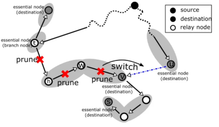
2) Grouping: Next, after the initial multicast tree is constructed, we now evaluate the Cost of every nodes in the tree by organizing the nodes in the tree into groups (the shade region in Fig. 2). The purpose of Grouping is that in the multicast tree, some nodes are essential nodes (e.g. destinations or branch nodes as in Fig. 2) must be reached, and others serve as relays. We group each essential node with relays on the path to the source until the next essential node. If node v switches its parent from node w to node u, the links(t,h),(h,w) and (w,v) can be pruned without influence on the connectivity of the multicast tree. We define the cost of node v as the gain of energy conservation after the pruning operation which can be calculated as:
cost(v) = (
Phw+ Pwv, if h is not the furthest
child of t
Phw+ Pwv+ (Pth− P2(t)), otherwise
WhereP2(t) is the transmitted power required to
support a link between t and the second furthest child of t.
Algorithm 2 Grouping
1: if v ∈ T receives ON REQ < s, S, m, x, σ, c > from a
neighbor u then
2: c← c + 1
3: if c= 1 then
4: status[v] ← head node
5: if v is the furthest child of u then
6: cost(v) ← P (u) − P2(u)
7: else 8: cost(v) ← 0 9: end if 10: else 11: σ← σ + P (u) 12: cost(v) = σ 13: end if
14: if (v is a (destination∨ branch node)) ∨ (c = m) then
15: status[v] ← tailnode
16: σ← 0
17: c← 0
18: end if
19: Send ON REQ < s, S, m, x, σ, c > to neighbors other than u in tree
20: end if
Fig. 2: Switch operation:
Node v switches its parent from node w to node u. And the relays which is no longer required after
switching are pruned.
2. After receiving all the CONST REP from every destinations, source then broadcasts Organize Nodes Request (ON REQ). An ON REQ message can be presented as a tuple< s, S, m, x, σ, c > consisted of the source nodes, the multicast session S, the group size limit m, the execution round demand x, the accumulative power consumption in current group σ and the number of nodes in current group c.
When a node v ∈ VT receives an ON REQ from
u, it updatesc immediately (line 2), and evaluates its cost (line 3-13), then checks whether it is the final node of the current group (line 14-18). Finally, it sends the request to neighbors other than u in the tree (line 19). We divide the tree into many groups by destinations and branch nodes. That is when node v is a destination in the multicast session or a branch node in the tree ,it will be the last node (tail node) in the current group (Fig. 3). There is another case that if we set the group size limit m ∈ N to bound the maximum group size, the group will also end at the node with c reach the group size limit m. The node also will be the tail node in the current group (Fig. 4). It then initialize σ and c to start a new group (line 15-17).
We evaluate the cost of nodes by accumulating power consumption of relays in the same group (line 11-12), but when the node is a starter (head node) of a group, the cost evaluation is different. The cost of such nodes is the power saved in the parent node when the node has been removed, as shown in line 5-8 of Algorithm 2.
Fig. 3: group size limit=∞
Fig. 4: group size limit=3
C. Refinement Step
After grouping, we had evaluated the cost of every nodeu ∈ VT. Then we can start the refinement
step. The refinement step is in a full localized fashion and can be organized as follow: every group has a token which is passed to nodes one by one in Relation Number order. The token passing from the tail node to the head node of a given group is called a round. A head node passes the token directly to the tail node in the same group to start a new round. This token can be regarded as a permission to do operations such as sending requests or initiating the refinement. Each group counts the number of round executed until it reaches the execution round demand x.
1) Token Passing: We initialize the refinement step by passing token from the tail node of the group. The algorithm of token passing is shown in Algorithm 3. Once a node v receives a token. It computes the Gain of all the nodeu ∈ N eighbor(v) withN umber(u) ≥ N umber(v)(Line 2-4). Gain(u) is given by Cost(v) − Increase(u). Here, Cost(v) had been evaluated during grouping, which can be seen as the accumulative power consumption required to sent data to node v. Increase(u) is the additional power needed at node u by adding a new child v, which is given in line 3. So the Gain is the amount of reduced power by switching the parent of node v to node u.
Algorithm 3 Token passing
1: if v receives token then
2: for all u such that u∈ N eighbor(v) ∧ N umber(u) ≥
N umber(v) do
3: Increase(u) = max{Pu,v, P(u)} − P (u)
4: Gain(u) = Cost(v) − Increase(u)
5: end for
6: if max
∀u {Gain(u)} > 0 ∧ N umber(u) = N umber(v)
then
7: send INR REQ to u and wait for reply
8: end if
9: if max
∀u {Gain(u)} > 0 ∧ N umber(u) > N umber(v)
then
10: send JOIN REQ< u, Gain(u), v > to u
11: if v is the head node of the group then
12: send LEAVE REQ< parent(v), v > to
par-ent(v)
13: end if
14: Wait for reply
15: end if
16: Pass the token to next node
17: end if
positive Gain is the same as node v, we send an Increase Number Request (INR REQ) first and wait for reply (line 6-8). The request will make node u increase its Relation Number under numbering principle, so node v can request node u to be its new parent. The details will be discussed later this section.
When the Relation Number of node u with high-est positive Gain is bigger then v. It can send the Join Request (JOIN REQ) to the node u to invite it to be its new parent(line 10). And if node v is the head node of its group, it also have to send a Leave Request (LEAVE REQ) to its parent (line 11-13). Then wait the reply for the request sent (line 14). Finally, after v receives all the reply, or there is no any node with positive Gain, it passes the token to the next node (line 16).
2) Request Handling: Now, we address how would a node respond to the received request. Due to the possibility of decision conflict, not all the switch refinement can be done immediately. To deal with the problem, every node should send a request and wait for acceptance before doing any switching operation.
The reply to the request under different situation is shown in Algorithm 4. When a node v receives a
JOIN REQ. If v had received the token this round, it is in a stable state. Which means this node won’t be pruned or decrease its emitting radius in this round. Accordingly, any node joining v won’t cause a conflict, and it can reply Join Request Acceptance (JOIN ACP) immediately (line 3-4).
But if v hasn’t received the token, we can’t assure whether v will be pruned in this round. So we hold the request by sending Join Request Hold (JOIN HOLD) back to u (line 6). Meanwhile, node v forwards the JOIN REQ along the tree path to the token node. The token node keeps track of the JOIN REQ with the largest Gain, JOIN REQ∗
. If the token node happens to be the originator of JOIN REQ∗
, a JOIN ACP will be transmitted. Otherwise, it transmits a JOIN RJT. Finally, the token is passed to the next node. The node receiving JOIN HOLD will hold the token until it also receiv-ing JOIN ACP, or Join Request Reject JOIN RJT.
When a node v receives a LEAVE REQ. Because the JOIN ACP and LEAVE ACP cause a conflict. If it had sent any JOIN ACP in this round, it replies Leave Request Reject (LEAVE RJT), else it replies Leave Request Acceptance (LEAVE ACP) (line 22-28).
3) Non-tree Node Operation: A node not in the tree can also contribute to energy saving by connecting two neighboring tree nodes through it. Unfortunately, limitation of space forbids full treat-ment of the subject. For more details, please consult our full paper[9].
4) Increase Number Request: Increase Number Request (INR REQ) is a special request, which is used to increase the number of a node in a reasonable range so that we can choose a new parent with the same Relation Number by sending INR REQ first.
After the computation of a token node v, if the Relation Number of the node u with largest Gain is as same as the token node v, we can send INR REQ to node u first to ask for increasing Relation Number under Numbering principle. When the node u receives the request, it can change its Relation Number to the average of current Relation Number and the upper bound of Relation Number. That is N umber(u) = (N umber(u) + upper bound of N umber(u))/2.
Algorithm 4 Request Handling
1: for a tree node v do
2: if v receives a JOIN REQ< v, Gain, u > then
3: if v has gotten token in this round then
4: reply JOIN ACP back to u
5: else
6: reply JOIN HOLD back to u
7: send JOIN REQ< v, Gain, u > to the token node
8: end if
9: end if
10: if v holds the token then
11: record the JOIN REQ with the largest Gain as JOIN REQ∗
12: if JOIN REQ< v, Gain, u > then
13: if JOIN REQ< v, Gain, u >= JOIN REQ∗
then
14: reply JOIN ACP back to u
15: else
16: reply JOIN RJT back to u
17: end if
18: else
19: pass the token to the next node
20: end if
21: end if
22: if v receives a LEAVE REQ< v, u > then
23: if v doesn’t send any JOIN ACP in this round then
24: reply LEAVE ACP back to u
25: else
26: reply LEAVE RJT back to u
27: end if
28: end if
29: end for
min{N umber(parent(u)), N umber(the node u requested if any)}. After node u changes its Relation Number, it then broadcasts the update message to all the neighbor, and sends a Increase Number Reply (INR REP) to node v. Accordingly, node v can request node u to be its new parent without violating numbering principle.
5) Refinement: If a head node receives both JOIN ACP and LEAVE ACP or a non-head node receives JOIN ACP. It can firstly perform the re-finement by switching to new parent node u. Then it sends Disorganize Nodes Confirm (DON CONF) to group members with bigger Relation Number. The node receives the message would regard itself as a non-tree node and relay DON CONF message to the next node until the message reaches a destination or a branch node. The former simply drops the
message and tags itself as a tail node. The later would send an ON REQ message to its child node to form a new group if it is no longer a branch node or drop the DON CONF message otherwise. If the pruned node had sent a JOIN HOLD before, it needs to send Join Request Reject (JOIN RJT) to cancel the hold. On the other hand, if the new parent u becomes a branch node, it turns itself into a tail node and all its children become head nodes of the corresponding groups. As a result, the switching and pruning operations retains a multicast tree structure.
V. PERFORMANCE EVALUATION
In this section, we evaluate the performance of LEMG through detailed simulation in static ad-hoc networks with our implemented c++ simulator. We assume the MAC layer is ideal and the radio transmission radius of a node is fixed to 250 meters. We use the energy model proposed by Ingelrest et al. [3], that is the power consumption of a emitter u with a radius ru is given by
PT(u) = ( r4 u+ 10 8 , if u is the source r4 u+ 10 8 +1 3(100) 4 , if u is a relay node 1 3(100) 4 , if u is a leaf node.
In each experiment, the ratio of number of the multicast group nodes to total nodes varies from 10% to 100% for every 10% increment, and we do 1000 simulation runs for each setting. The nodes in the network is uniformly distributed inside a square region and the network connectivity is assured. Besides, the nodes in the multicast group are chosen randomly as well as the source node.
The experiments can be divided into two stages. In the first stage, we investigate the influence of two important settings of LEMG: group size limit m and execution round demand x. In the second stage, we compare LEMG with other protocols to evaluate the performance.
A. Performance Metrics
In each experiment, we look into the following metrics for evaluating the performance of LEMG with respect to other representative algorithms.
1) Total power consumption (TPC): The total tree power required using a heuristic algo-rithm. It is the average of the sum of the energy consumed in every tree node for one
unit of transmission out of 1000 simulation runs.
2) Relative TPC: The ratio of the TPC of LEMG to that of the initial multicast tree SPT. 3) Normalized TPC: The ratio of TPC to
the average of the best tree powers ob-tained from heuristic algorithms in the set H = {MIP,DMEM,LEMG}. That is, Normal-ized T P C = T P Calg
T P Cbest, where T P Cbest =
avg min{T P Calg} and alg ∈ H.
4) Total control messages (TCM): The number of control messages for refinement over the whole course of simulation. The metric can be used to evaluate the message complexity of heuristic algorithms.
5) Total time periods (TTP): The total time periods required for a simulation run of a heuristic algorithm. A time period is defined as the processing time and transmission time of a node. The metric can be viewed as a measure of execution time of the correspond-ing algorithm in an ideal environment with collisionless MAC layer.
B. Experiments Result in different settings
In the first stage of experiments, an ad-hoc net-work with 400 nodes in a physical area of 2000 meters × 2000 meters is simulated. All curves are averages over 1000 independent simulation runs.
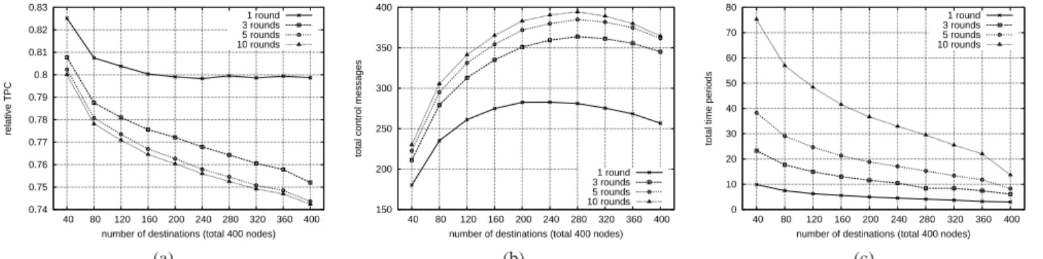
1) Execution Round Demand: At first, the influ-ence of execution round demand x is studied. The group size limit m is set to 400 which means no restriction on group size. Generally speaking, more refinement could possibly be discovered with larger x. As shown in Fig. 5a, the relative power consump-tion decreases with the increase of x. However, the relative power consumption when x=10 is similar to that when x=5. In Fig. 5b, the TCM are similar under x=10 and x=5 which represents the number of refinement can be done is very limited after five rounds of execution in each group. But, as we can see in Fig.5c, the TTP when x=10 is approximately twice of that when x=5. Consequently, we adopt the setting x=5 in all the following experiments.
2) Group Size Limit: Next, we analyze the im-pact of group size m. It imposes a restriction on the maximal hops of message passing for one refine-ment operation. Consider the Grouping mechanism,
more redundant relay nodes and links in between could be removed with larger m, resulting in better energy conservation. On the other hand, a large group size can cause the increase in the commu-nication overhead and thus the time complexity of the algorithm. Our focus is to find an appropriate setting for m through extensive simulations.
Fig. 6a shows the relative power consumption of multicast trees constructed by our LEMG with different setting of m. Each curve is characterized by the multicast group size. We can observe that the larger the m, the lower the power consumed. Meanwhile, no more improvement can be made when m is larger than ten. Fig. 6b and Fig. 6c also show the TCM and the TTP are nearly the same when m=10 and m=400(i.e. no restriction on group size). Therefore, we set m=10 in all the following experiments.
C. Performance Result
After the values of x and m have been decided, we compare our LEMG with MIP and DMEM. MIP is perhaps the most well-known centralized multicast algorithm and has been often used as a baseline algorithm for comparison. DMEM, to the best of our knowledge, is the latest distributed tree-based multicast algorithm that attempts to explore the energy conservation by the use of several localized operations.
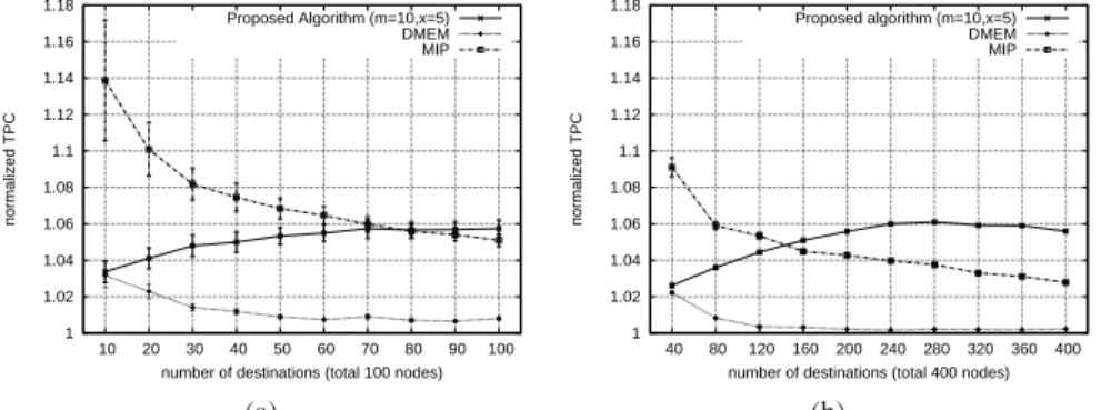
The performance is evaluated on two different network scenarios. For one is the standard scenario where 100 nodes are randomly generated in a square area of size 1000 meters × 1000 meters. The other is the large-scale scenario, there are 400 nodes in the square region of 2000 meters × 2000 meters. Fig. 7a and Fig. 7b show the normalized power consumption with respect to various multicast group sizes for the standard scenario and the large-scale scenario respectively. LEMG performs almost as good as DMEM and better than MIP when the multicast group size is small. As the multicast group size increases, LEMG is less energy efficient. This is because the average group size in a LEMG tree decreases with the growth of multicast group size. However, it is only 5% − 6% worse than DMEM at most.
Fig. 8a and Fig. 8b depict the comparison of total control messages (TCM) which is shown on the
0.74 0.75 0.76 0.77 0.78 0.79 0.8 0.81 0.82 0.83 40 80 120 160 200 240 280 320 360 400 relative TPC
number of destinations (total 400 nodes) 1 round 3 rounds 5 rounds 10 rounds (a) 150 200 250 300 350 400 40 80 120 160 200 240 280 320 360 400
total control messages
number of destinations (total 400 nodes) 1 round 3 rounds 5 rounds 10 rounds (b) 0 10 20 30 40 50 60 70 80 40 80 120 160 200 240 280 320 360 400
total time periods
number of destinations (total 400 nodes) 1 round 3 rounds 5 rounds 10 rounds
(c)
Fig. 5: Execution rounds experiment (a) Relative power consumption (b) Total control messages (c) Total time periods 0.74 0.76 0.78 0.8 0.82 0.84 0.86 0.88 1 2 3 4 5 6 7 8 9 10 relative TPC
group size limit (m) 40/400 destinations 120/400 destinations 200/400 destinations (a) 100 150 200 250 300 350 400 40 80 120 160 200 240 280 320 360 400
total control messages
number of destinations (total 400 nodes) m=2 m=4 m=6 m=10 m=400 (b) 5 10 15 20 25 30 35 40 40 80 120 160 200 240 280 320 360 400
total time periods
number of destinations (total 400 nodes) m=2 m=4 m=6 m=10 m=400 (c)
Fig. 6: Group sizes experiment (a) Relative power consumption (b) Total control messages (c) Total time periods
vertical axis in log scale for LEMG and DMEM. We can observe that the message complexity of DMEM grows dramatically with the multicast group size and the network size. This is due all the local energy savings information has to be sent to the source and the final decision will be send back to the node with the maximum energy savings. On the contrary, LEMG has much lower TCM and it grows linearly with network sizes.
The comparison of the total time periods (TTP) of LEMG and DMEM under different network sce-narios are shown on Fig. 9a and Fig. 9b. The x-axis represents various multicast group sizes and the TTP is shown on the y-axis in log scale. We can see that in DMEM, the TTP increases with multicast group sizes, while that of LEMG decreases in contrast. It is due to larger multicast group results in smaller groups in the LEMG tree and the execution time is therefore reduced. Furthermore, the TTP is almost
invariant to network sizes, while in DMEM, the TTP increases dramatically with network sizes.
In summarize, although LEMG is slightly inferior to DMEM in energy conservation under large mul-ticast group size, its superiority on TCM and TTP over DMEM is obvious. When considering node mobility and varying link condition in wireless ad-hoc networks, timeliness of the algorithm is impor-tant. Otherwise, the energy savings information may not be valid anymore. From the simulation results, LEMG is more suitable to be applied in a large-scale ad-hoc wireless network.
VI. CONCLUSION ANDFUTURE WORK
In this work, we proposed a fully localized refine-ment based algorithm for building energy-efficient multicast tree in wireless ad hoc network. We started with the construction of a SPT on top of ESPT. With Grouping mechanism, we make the cost evaluation
1 1.02 1.04 1.06 1.08 1.1 1.12 1.14 1.16 1.18 10 20 30 40 50 60 70 80 90 100 normalized TPC
number of destinations (total 100 nodes) Proposed Algorithm (m=10,x=5) DMEM MIP (a) 1 1.02 1.04 1.06 1.08 1.1 1.12 1.14 1.16 1.18 40 80 120 160 200 240 280 320 360 400 normalized TPC
number of destinations (total 400 nodes) Proposed algorithm (m=10,x=5)
DMEM MIP
(b)
Fig. 7: Normalized power consumption comparison of MIP, DMEM and LEMG (a) Standard scenario (b) Large-scale scenario 10 100 1000 10000 10 20 30 40 50 60 70 80 90 100
total control messages
number of destinations (total 100 nodes) Proposed algorithm DMEM (a) 100 1000 10000 100000 40 80 120 160 200 240 280 320 360 400
total control messages
number of destinations (total 400 nodes) Proposed algorithm DMEM
(b)
Fig. 8: Total control messages comparison of DMEM and LEMG (a) Standard scenario (b) Large-scale scenario 1 10 100 1000 10 20 30 40 50 60 70 80 90 100
total time periods
number of destinations (total 100 nodes) Proposed algorithm DMEM (a) 1 10 100 1000 10000 40 80 120 160 200 240 280 320 360 400
total time periods
number of destinations (total 400 nodes) Propose algorithm
DMEM
(b)
Fig. 9: Total time periods comparison of DMEM and LEMG (a) Standard scenario (b) Large-scale scenario
and limit the hop count of message passing in the refinement step. Two adjustable parameters: group size limit m and execution round demand x control the time required for refinement and the efficiency of LEMG. Besides, All the message passing is within a constant hop count which is decided by m.
The simulation results show the average total
power consumption of LEMG is colse to DMDM with only 5% difference while all the message passing in proposed algorithm is limit to m hops. Besides, the refinement of LEMG can be done in only limited hops of message passing and nearly constant regardless of the network size and the number of destinations in the same setting. What is more, the total control message in the refinement
grows only linearly with network size, so the aver-age control messaver-age per node is also not affected by network size. Consequently, the algorithm we proposed can achieve energy-efficient comparable solution to others in only few hops message passing, and can be adapted well in any size of network due to the localized property.
Most energy-efficient multicast algorithm only consider an ideal MAC layer. For future work, we shall implement the performance evaluation in net-work simulator to study a more realistic MAC layer. We shall also evaluate the influence of mobility and directional antenna on LEMG for a more piratical scenario.
REFERENCES
[1] M. Cagalj, J.-P. Hubaux, and C. Enz. Minimum-energy broad-cast in all-wireless networks: NP-completeness and distribution issues. In Proc. of the ACM MobiCom, pages 172–182, 2002. [2] J. Cartigny, D. Simplot, and I. Stojenovic. Localized minimum-energy broadcasting in ad-hoc networks. In Proc. of the IEEE
INFOCOM, volume 3, pages 2210– 2217, 2003.
[3] J. Cartigny, D. Simplot, and I. Stojmenovic. Optimal transmis-sion radius for energy efficient broadcasting protocols in ad hoc andsensor networks. In IEEE Trans. on Parallel and Distributed
Systems, volume 17, pages 536–547, 2006.
[4] S. Guo, V. Leung, and O. Yang. A scalable distributed multicast algorithm for lifetime maximization in large-scale resource-limited multihop wireless networks. In Pro. of the
IEEE International Conference On Wireless communications and mobile computing (IWCMC), pages 419–424, 2006.
[5] S. Guo and O. Yang. A dynamic multicast tree reconstruction algorithm for minimum-energy multicasting in wireless ad hoc networks. In Proc. of the IEEE International Performance
Computing and Comm. Conf. (IPCCC), pages 637–642, 2004.
[6] S. Guo and O. Yang. Localized operations for distributed mini-mum energy multicast algorithm in mobile ad hoc networks. In
IEEE Trans. on Parallel and Distributed Systems, volume 18,
pages 186–198, 2007.
[7] S. Guo and O. W. Yang. Energy-aware multicasting in wireless ad hoc networks: A survey and discussion. In Computer
Communications, volume 30, pages 2129–2148, 2007.
[8] P.-C. Hsiu and T.-W. Kuo. A Maximum-Residual Multicast Protocol for Large-Scale Mobile Ad Hoc Network. In IEEE
Trans. on Mobile Computing, 2009.
[9] T.-H. Huang. Fully Localized Energy-Efficient Multicast in Wireless Ad Hoc Network. In Master thesis,National Taiwan
University, 2009.
[10] F. Ingelrest and D. Simplot-Ryl. Localized broadcast incremen-tal power protocol for wireless ad hoc networks. In Proc. of the
IEEE Symposium on Computers and Communications (ISCC),
pages 28–33, 2005.
[11] N. Li and J. C. Hou. Blmst: A scalable, power-efficient broadcast algorithm for wireless networks. In Proc. of the IEEE
International Conf. on Quality of Swevice in Heterogeneous Wired/Wireless Networks (QSHINE), pages 637–642, 2004.
[12] X.-Y. Li, W.-Z. Song, and W. Wang. A unified energy-efficient topology for unicast and broadcast. In pro. of the ACM
MobiCom, 2005.
[13] P. M. Mavinkurve, H. Q. Ngo, and H. Mehra. Mip3s: Algo-rithms for power-conserving multicasting in static wireless ad hoc networks. In Pro. of the IEEE Internorional Conference
on Networks (ICON), 2003.
[14] A. Orda and B.-A. Yassour. Maximum-lifetime routing al-gorithms for networks with omnidirectional and directional antennas. In Proc. of the ACM MobiHoc, pages 426–437, 2005. [15] B. Wang and S. K. Gupta. On maximizing lifetime of multicast trees in wireless ad hoc networks. In Pro. of the IEEE
International Conference on Parallel Processing, pages 333–
340, 2003.
[16] B. Wang and S. K. S. Gupta. S-remit: A distributed algorithm for source-based energy efficient multicasting in wireless ad hoc networks. In Proc. of the IEEE GLOBECOM, pages 3519– 3524, 2003.
[17] S.-C. Wang, D. S. Wei, and S.-Y. Kuo. An SPT-based Topology Control Algorithm for Wireless Ad Hoc Networks. In Computer
Communications, volume 29, pages 3092–3103, 2006.
[18] J. E. Wieselthier, G. D. Nguyen, and A. Ephremides. On the construction of energy-efficient broadcast and multicast trees in wireless networks. In Proc. of the IEEE INFOCOM, pages 585–594, 2000.