Image Compression Using Grey-Based Neural Networks In the Wavelet Transform Domain

全文

(1)Image Compression Using Grey-Based Neural Networks In the Wavelet Transform Domain Chi-Yuan Lin and Chin-Hsing Chen Department of Electrical Engineering, National Cheng Kung University, Tainan, 70101 Taiwan, R.O.C. E-mail: [email protected], [email protected] Abstract. an important role in image compression. The wavelet transform is identical to a hierarchical. The wavelet transform has recently emerged. as. a. powerful. tool. for. subband. system.. Basically,. the. wavelet. image. transform decomposes an image into a set of. compression. In this paper, the Grey theory is. sub-image blocks that are more stationary and. applied to a two-layer modified Competitive. hence provide better coding performance. A. Learning Network (GCLN) to generate optimal. higher compression ratio can be achieved by the. solutions for VQ. In accordance with the degree. exploitation of quantizers adapted to the. of similarity measures between training vectors. statistics of the sub-image blocks.. and codevectors, the grey relational analysis is. A number of vector quantization algorithms. used to measure the relationship degree among. for data compression have proposed over the. them. The input image is first decomposed into. years [3-5]. The purpose of vector quantizaton is. four subbands in the 1-level wavelet transform.. to create a codebook such that the average. Then the corresponding transformed coefficients. distortion between training vectors and their. are trained using GCLN to form individual. corresponding codevectors in the codebook is. codebooks for each subband. The compression. minimized. Codebook design can be considered. performances using the proposed approach are. as a clutering process in which each training. compared with GCLN and the conventional. vector is classified to a specific class. The. vector quantization LBG method. Experimental. clustering. results show that promising performance can be. iteratively such that the average distortion. obtained. between training vectors and codevectors in the. using. the. GCLN. with. wavelet. decomposition. Key words: learning. updates. the. codebook. codebook becomes smaller and smaller.. Image compression, Competitive. network,. process. Grey. theory,. Wavelet. transform.. Neural networks with competitive learning have been demonstrated capable of performing vector quantization [6-8]. In addition to the neural network-based techniques, the grey. 1. Introduction. relational theory proposed in 1982 [9-12] has also been demonstrated to address the codebook. In recent years, wavelet coding [1-2] plays. design in this paper. In Grey-based Competitive.

(2) Learning Network (GCLN), the learning rule. interconnection. strength.. In. conventional. and stopping criterion of the original competitive. competitive learning only one output unit is. learning neural network are modified to address. active at a time and the objective function is. the codebook design using the grey relational. given by. strategy. The problem of VQ is regarded as a minimization process of an object function. This object function is defined as the average. Jc =. 1 2. c. n. ∑∑ u. i, j. xi −ω j. 2. (1). j =1 i =1. distortion between the training vectors in a divided image to the cluster centers represented. where n and c are the number of training vectors. by the codevectors in the codebook. The. and the number of clusters respectively. ui , j = 1. modified. is. if x i belongs to cluster j and ui , j = 0 for. simpler than that of the conventional competitive. all other clusters. The neuron that wins the. leaning network, and is constructed as a. competition is called the winner-take-all neuron.. two-layer fully interconnected array with the. Thus ui , j indicates whether the input sample. input neurons representing the training vectors. x i activates neuron j to be a winner. ui , j is. and output neurons representing the codevectors. given by. competitive. learning. network. in the codebook.. decomposed into four subbands LL1, LH1, HL1,. 1 if x i − ω j ≤ xi − ωk , for ui , j =  0 otherwise.. and HH1 in the 1-level wavelet transform. Then. (2). In this paper, the input image is first. all. k ;. the corresponding transformed coefficients are trained. using. codebooks. for. GCLN each. to. form. individual. subband.. Computer. simulations show that the GCLN used with VQ is promising for image compression.. The incremental ∆ω j is given by [13-14]. ∆ω j = −η. n ∂J c x i − ω j u i, j , =η ∂ω j i =1. ∑(. ). j = 1,2, L , c.. (3.a). 2. Competitive Learning Network where A competitive learning network is an. η. is. the. samples,. based on similarity measure over the feature. incrementally, i.e.. only if it wins the competition among all. parameter.. Although Eq. (3.a) is written as a sum over all. unsupervised network which selects a winner. space. A proper neuron state is updated if and. learning-rate. practically. (. it. ). is. usually. ∆ω j = η xi − ω j ui , j , j = 1,2,L, c.. used. (3.b). neurons. Many schemes for competitive learning networks have been proposed [13-14].. The updating rule is given by. In the simple competitive learning network, the single output layer consists of cluster centers, each of which is fully connected to the inputs via. ω j (t + 1) = ω j (t ) + ∆ω j (t ) .. (4).

(3) The. Modified. Competitive. Learning. distortion is at the minimum value. The average. E[d (x i , ω j )]. between. an. input. Network (MCLN) has the same architecture as. distortion. the conventional competitive learning network.. sequence of training vectors {x i , i = 1,2,..., n}. It is an unsupervised competitive learning. and its corresponding output sequence of code. network using the modified competitive learning. vectors {ω j , j = 1,2,..., c} is defined as. rule and stopping criterion. Similar to the standard competitive learning rule in Eqs. (3.b) and (4), the least squared error solution can be. D = E[d (x i ,ω j )] =. 1 n. n. ∑ d ( x ,ω i. j). (6). i =1. obtained by [13] The grey system is usually divided into ω (t) +η(xi −ωj ) if xi −ωj ≤ xi −ωk , for all k ; ωj (t +1) =  j . ωj (t) otherwise . several topics such as grey theory, grey. (5). space, grey decision, and grey relational analysis.. mathematics, grey prediction, grey generating. Grey. relational. theory. demonstrates. the. The MCLN algorithm modifies only output. measurement of similarity between training. neurons without updating the interconnection. vectors and codevectors based on the grey. strengths.. the. relational space. Let x i be a training vector. the. and ω. Instead. interconnection. of. updating. strengths. using. winner-take-all scheme in the conventional. be the codevector j, then the grey. j. relational coefficient is defined as. competitive learning network and for the purpose of simplifying the hardware architecture, the MCLN only modifies the output states. (. γ x i ,ω. j. )=. ∆ min . + ξ ∆ max ∆ ij + ξ ∆ max .. .. (7). (cluster centroids). where. 3. Grey-Based Competitive Learning Network for VQ Suppose an image is divided into. n. blocks (vectors of pixels) and each block occupies l × l pixels. A vector quantizer is a technique. that. maps. the. Euclidean. l × l -dimensional space. R l×l. into a set. ∆ min . = min x i − ω j ∆ max . = max x i − ω j ∆ ij = x i − ω j and 0 < ξ < 1 is the distinguished coefficient. The grey relational grade is given by. {ω j , j = 1,2,..., c} of points in R l×l , called a codebook. It looks for a codebook such that each. γ i, j =. 1 l×l. l×l. ∑ γ (x ,ω ) i. j. (8). m =1. training vector is approximated as close as possible by one of the code vectors in the. where m is the dimension of the training vector. codebook. A codebook is optimal if the average. x i and the codevector ω j ..

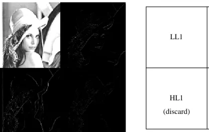
(4) In this paper, the grey theory is applied to. any function satisfying the scaling equation. a two-layer MCLN in order to generate optimal solution for VQ. The modified competitive. Φ (x ) =. ωj (t) +η(xi −ωj ) if ωj (t +1) = ωj (t) . ∑ c Φ(2 x − i ). (11). i. i∈Z. learning rule is modified as. γi, j ≥γi,k , for all k ; . otherwise. For any integer j, we define vector space V. as. follows. (9) V. j. {. }. (. ). = span Φ ij (x ). The steps of codebook design using the grey-based competitive learning network are. j. (12). Φ ij (x ) = Φ 2 j x − i ,. i∈Z. (13). given as follows. Step 1: Initialize the codevectors ω j (2 ≤ j ≤ c ) ,. If. V. j. satisfies. the. following. four. learning rate η , maximum error (ME),. multiresolution analysis conditions. total error (TE), and a threshold value. Condition 1: f (x )∈ V j ⇔ f 2 − j x ∈ V 0 , ∀j ∈ Z. ε. Step 2: Input a training vector x i and find the winner’s. codevector. based. on. the. (. Condition 2:. I. i∈Z V. i. = {0}. Condition 3:. U. i∈Z V. i. = L2 (R ). maximum grey relational grade.. ). Step 3: Apply Eq. (9) to update the winner’s. Condition 4: L ⊂ V −2 ⊂ V −1 ⊂ V 0 ⊂ V 1 ⊂ V 2 ⊂ L. codevector and set TE=TE+ ∆ ij .. it is easy to show that the mother function of. Step 4: Repeat Steps 2 and 3 for all input samples, then if (ME − TE ). ME. < ε , go. wavelets is given by Ψ (x ) =. ∑ (− 1) c i. 1−i Φ. (2 x − i ). (14). i∈Z. to step 5; otherwise replace ME content from TE, and go to Step 2. Step 5: Complete the codebook design.. One of the most important characteristics of the wavelet transform is multiresolution. The. 4. Wavelet Transform and GCLN. wavelet transform converts the pixel values of images to wavelet domain, without lose any. signal. information in the spatial domain. A wavelet. decomposition technique [16]. The mother. decomposition of Lena image using the 1-level. function of wavelets, Ψ (x ) , can be any function. Haar basis wavelet transform is shown in Fig. 1.. The. wavelet. transform. is. a. Vector quantization has been demonstrated. if it satisfies the following condition. ∫. ∞. −∞. to be an efficient method for image compression.. 2. Ψ (x ) dx < ∞. (10). The motivation for the proposed GCLN with. Basically, most of the mother functions are. wavelet decomposition scheme is based upon the. derived from the scaling function Φ(x) which is. fact. that. the. lower. resolution. wavelet.

(5) coefficients hold more information and higher resolution. wavelet. coefficients. hold. less. information. The basic idea is described as follows. The 1-level wavelet transform is first performed on the input image to generate the. PSNR = 10 log10. 255 2 MSE. (15). and MSE =. 1 N. 2. ∑ ∑ (x N. ) − xij. N. i =1. j =1. ij. ). 2. (16). corresponding transformed coefficient. Then, the coefficients of each scale are trained separately. where xij and xˆ ij are the pixel gray levels. to obtain an individual codebook. For example,. from the original and reconstructed images, and. as shown in Fig. 2, the coefficients of LL1 and. 255 is the peak gray level. Table 1 shows the. LH1 are divided into the blocks of size 2 × 2 and. PSNR and MSE of the “F16”, “Girl” and “Lena”. 4 × 4 from which two codebooks of size = 512,. images reconstructed from three codebooks of. and 64 were built respectively. The coefficients. size 64, 128, and 256 designed by the LBG and. of HL1 and HH1 are totally discarded since they. the. rarely hold information, and are reconstructed by. decomposition. The comparison between GCLN. searching the best-matched codevectors from the. without decomposition (named GCLN) and. codebook of LH1. The GCLN is eventually. GCLN with wavelet decomposition (named by. employed as vector quantization technique of. WT+GCLN) is shown in table 2. In table 2, the. image compression and thus reducing bit rate. compression. ratio. (CR). and training time.. (CR_LH1. ×. 3)]. 5. Experimental Results. GCLN. methods. without. is. wavelet. [CR_LL1. +. 4. =. /.  2× 2×8 4× 4×8  + × 3  ÷ 4 = 16.89  9 6   WT+GCLN,. and. Codebook design is a primary problem in. for. 4×4×8 = 21.33 6. In this paper, the quality of the images. 4× 4×8 = 18.29 , 7. reconstructed from the designed codebooks was. respectively. From the experimental results, the. compared with that from the LBG and GCLN. reconstructed images obtained from the GCLN. methods. The training vectors were extracted. are superior to those obtained from the LBG. from 256 × 256. with 8-bit gray level real. algorithm, and those from the WT+GCLN are. images, each of which is divided into 4 × 4. significantly better than those from the GCLN. blocks to generate 4096 non-overlapping 16-D. algorithm.. image compression based on vector quantization.. 4× 4×8 = 16 8. ,. for GCLN. training vectors. Three codebooks of size = 64, 128, and 256 were built by these training vectors. The. resulting. images. were. 6. Conclusions. evaluated. subjectively by the mean squared error (MSE). In this paper, a two-layer modified. and peak signal to noise ratio (PSNR) defined. competitive learning neural network based on. for images of size N×N as. gray relational theory for VQ in wavelet transform domain has been presented. Instead of.

(6) updating the interconnection strengths using the. The Fifth Symposium on Computer and. winner-take-all scheme in the conventional. Communication Technology, pp. 1B-11~ 1B. competitive. -15, 2000.. learning. network,. the. GCLN. algorithm only modifies output neurons and. [8] C. Y. Lin, C. H. Chen, and J. S. Lin, “VQ. omits the updating of the interconnection. Codebook. strengths. Experimental results show that the. Competitive Learning Network,” The 13th. GCLN. IPPR Conference on Computer Vision,. and. reconstructed. WT+GCLN images. methods. better. than. produce those. reconstructed by the LBG method.. Graphics. Design. and. Using. Image. a. Genetic. Processing,. pp.. 362-369, 2000. [9] J. L. Deng, “Properties of Relational Space. References. for Grey System,” Grey System, Beijing, China Ocean Press, 1988.. [1] M. Antonini, M. Barlaud, P. Mathieu, and I.. [10] J. L. Deng, “Introduction to Grey Systems. Daubechies, “Image Coding Using Wavelet. Theory,” The Journal of Grey System, Vol.1. Transform,” IEEE Trans. Image Processing,. No.1, pp. 1-24, 1989. [11] H. C. Huang and J. L. Wu, “Grey System. Vol.1, pp. 205-220, 1992. [2] R. A. Devore, B. Jawerth, and B. J. Lucier,. Theory on Image Processing and Lossless. Wavelet. Data Compression for HD-media,” The. Transform Coding,” IEEE Trans. Informat.. Journal of Grey Theory & Practice, Vol. 3,. Theory, Vol. 38, pp.719-746, 1992.. No. 2, pp.9-15, 1993.. “Image. Compression. through. [3] Y. Linde, A. Buzo, and R. M. Gray, “An. [12] Y. T. Hsu and J. Yeh, “Grey-Base Image. Algorithm for Vector Quantizer Design,”. Compression,” The Journal of Grey system,. IEEE Trans. Commun., Vol. COM-28, pp.. Vol. 2, pp. 105-120, 1998. [13] C. C. Jou, “Fuzzy Clustering Using Fuzzy. 85-94, Jan., 1980. [4] R. M. Gray, “Vector Quantization,” IEEE. Competitive Learning Networks,” Neural Networks,. ASSP Magazine, Vol.1, pp. 4-29, 1984.. IJCNN.,. International. Joint. [5] A. Gersho, and R. M. Gray, Vector. Conference on , Vol. 2 , pp. 714 –719, 1992.. Quantization and Signal Compression,. [14] J. S. Lin, K. S. Cheng, and C. W. Mao,. Kluwer Academic Publishers, Norwell, Ma.,. “Segmentation of Multispectral Magnetic. 1992.. Resonance Image Using Penalized Fuzzy. [6] E. Yair, K. Zeger, and A. Gersho, “Competitive. Learning. and. Soft. Competition for Vector Quantizer Design,” IEEE Trans. Signal Processing, Vol. 40, pp. 294-309, 1992. [7] C. H. Chen, C. Y. Lin, and J. S. Lin, “A Compensated Fuzzy Competitive Learning Network Applied on Image Compression,”. Competitive. Learning. Network,”. Computers and Biomedical Research 29, pp.314-326, 1996. [15] 戴顯權, “資料壓縮”, 松崗, 1996..

(7) Fig. 1 1-level wavelet transformed. LL1. LH1. HL1. HH1. (discard). (discard). Fig. 2 1-level wavelet transformed. Lena image (Haar basis). four subbands. Table 1. PSNR and MSE of the images reconstructed from codebooks of various size designed by the LBG and proposed GCLN algorithms. Codebook 64. 128. 256. Sizes PSNR. MSE. PSNR. MSE. PSNR. MSE. Images/Algorithms LBG. 24.11. 222.31. 25.29. 192.30. 26.34. 142.94. GCLN. 24.75. 217.68. 25.35. 189.69. 26.64. 140.90. LBG. 27.68. 109.62. 28.51. 91.60. 29.69. 77.09. GCLN. 28.79. 85.98. 29.91. 66.44. 31.05. 51.02. LBG. 25.26. 146.89. 26.37. 127.01. 27.06. 106.71. GCLN. 26.09. 160.01. 27.23. 123.11. 28.84. 84.89. F16. Girl. Lena. Table 2. PSNR and MSE of the images reconstructed from various compression ratios (CR) designed by the GCLN and WT+GCLN methods. Images F16 PSNR. Girl MSE. PSNR. Lena MSE. PSNR. MSE. Algorithms/CR GCLN. CR=21.33. 24.75. 217.68. 28.79. 85.98. 26.09. 160.01. WT+GCLN. CR=16.89. 26.64. 140.90. 31.31. 48.10. 28.91. 83.51. GCLN. CR=18.29. 25.35. 189.69. 29.91. 66.44. 27.23. 123.11. WT+GCLN. CR=16.89. 26.64. 140.90. 31.31. 48.10. 28.91. 83.51. GCLN. CR=16. 26.64. 140.90. 31.05. 51.02. 28.84. 84.89. WT+GCLN. CR=16.89. 26.82. 135.27. 31.31. 48.10. 28.91. 83.51.

(8) Image Compression Using Grey-Based Neural Networks In the Wavelet Transform Domain 應用灰色理論的神經網路於小波轉換域之影像壓縮技術 Chi-Yuan Lin (林基源) and Chin-Hsing Chen (陳進興) 國立成功大學電子工程研究所 E-mail: [email protected] [email protected]. 摘要小波轉換合併影像壓縮技術近來已成為有力的工具。本篇論文㆗，灰色理論被應用到㆒個兩層的修正競爭式學習網路㆖。其目的在於建立㆒編碼簿使得介於訓練向量與編碼簿㆗之編碼向量的灰關聯度最大。輸入影像首先用小波轉換將其分解成㆕個次頻帶，然後其對應的小波轉換係數再應用灰關聯度的修正競爭式學習網路對個別次頻帶訓練編碼簿。根據實驗結果顯示，基於灰色理論最大關聯準則之修正競爭式學習網路於小波轉換域㆖所產生的影像壓縮編碼簿具有良好的效能。關鍵字：影像壓縮 (Image compression)，競爭學習網路 (Competitive learning network)，灰色理論 (Grey theory)，小波轉換 (Wavelet transform)。.

(9)