國 立 交 通 大 學
資訊科學與工程研究所
碩
士
論
文
以時空資料探勘技術找出都會區交通路網瓶頸點的
模式
A Spatiotemporal Traffic Bottleneck Mining Model for
Discovering Bottlenecks in Urban Network
研 究 生:陳曉涵
指導教授:曾憲雄 博士
ii
以時空資料探勘技術找出都會區交通路網瓶頸點的模式
A Spatiotemporal Traffic Bottleneck Mining Model for Discovering
Bottlenecks in Urban Network
研 究 生:陳曉涵 Student: Hsiao-Han Chen
指導教授:曾憲雄博士 Advisor: Dr. Shian-Shyong Tseng
國 立 交 通 大 學
資 訊 科 學 與 工 程 研 究 所
碩 士 論 文
A Thesis
Submitted to Institute of Computer Science and Engineering College of Computer Science
National Chiao Tung University in partial Fulfillment of the Requirements
for the Degree of Master
In
Computer Science
June 2007
Hsinchu, Taiwan, Republic of China
iii
以時空資料探勘技術找出都會區交通路網瓶頸點的
模式
學生: 陳曉涵 指導教授: 曾憲雄 博士 交通大學資訊科學與工程研究所摘要
因為都市化及交通工具的普及,交通擁塞情形也越來越嚴重,尤其是都 會區,許多研究因而提出來改善交通擁塞的問題,其中找到交通瓶頸點對於 改善交通擁塞將會是非常有效且重要的議題。因為高速公路路網比都會區路 網相對簡單的多且高速公路的瓶頸點大部分就位於閘道附近,所以大多數交 通瓶頸點的相關研究都在高速公路。又因為都會區路網的瓶頸點是會隨著時 間而改變的,所以找到都會區交通瓶頸點變成是一項非常困難但卻非常重要 的任務。所以我們提出了一個時空交通瓶頸點探勘模組(Spatiotemporal Traffic Bottleneck Mining Model, STBM)利用資料探勘方式加上我們提出 的三個瓶頸點特徵來找到都會區路網瓶頸點。我們的實驗設計在台北都會 區,利用即時的計程車派遣系統(Taxi Dispatch System)來收集交通資訊, 收集時間為 2006/02 到 2007/03。從實驗結果可以看出,STBM 的帄均準確率 確實比傳統統計法的略高,幾乎有高達近八成。而且分布結果相當帄均也比 較穩定。未來我們將會整合現有的 STBM 加上歷史的交通資訊以及即時交通資 訊,發展一個新的交通瓶頸點及時預測系統,用以提供用路人或交通管理者 更多及時有效的資訊。 關鍵字: 智慧型運輸系統, 定位資訊系統, 計程車派遣系統, 交通瓶頸點, 時空資料探勘iv
A Spatiotemporal Traffic Bottleneck Mining Model
for Discovering Bottlenecks in Urban Network
Student: Hsiao-Han Chen Advisor: Dr. Shian-Shyong Tseng Department of Computer Science
National Chiao Tung University
Abstract
The occurrence of traffic congestion has been increasing around world-wide as the result of the increasing of motorization, urbanization, population growth and changes in population density, especially in Urban Network; therefore, many researches are proposed to improve the traffic congestion; moreover, finding the traffic bottlenecks is the most important thing to improve the traffic congestion. As we know, freeway bottlenecks are always fixed and well known as gateway but the urban network bottlenecks may vary with spatial and temporal environment; therefore, finding out urban network bottleneck becomes a very difficult but very important mission. We propose a Spatiotemporal Traffic Bottleneck Mining Model (STBM) in this thesis to discover the urban network bottlenecks based on three heuristics we developed.
In this thesis, STBM prototype model is implemented based on a real time LBS-based application to find out the Taipei urban network bottlenecks. Experimental results show that the average accuracy in workday of STBM is up to 80% and it‟s better than the traditional statistic model. In the near future, the STBM model could be implemented as a real time bottleneck detection and prediction system, which integrates the historical traffic patterns and real-time traffic information.
Keyword: Intelligent Transportation System, Location Based Service, Traffic
v
致謝
首先誠摯的感謝指導教授:曾憲雄博士。曾教授在這兩年碩士生涯中, 對我們的細心教導以及諄諄教誨,不管在學習研究方面抑或是做人處事,時 常與我們分享他過去寶貴的經驗,也在我感到迷惘時給予當頭棒喝,真的非 常感謝曾教授給予我們的耐心、用心及苦心,讓學生獲益匪淺,特別要在這 對教授獻上十二萬分的感謝。接著要特地感謝卓訓榮教授,在論文研究期間, 不厭其煩的給予我非常多的建議及協助,也特別撥冗來參加學生的論文口試 審查,讓我的論文更加完整,非常謝謝您。同時也要非常感謝王景弘博士以 及洪宗貝教授在學生口試時特別撥空來參加審查,也給予我非常多的建議及 鼓勵,讓本篇論文更加豐富、更加有價值。 在研究生涯中,也非常感謝李威勳學長,謝謝您這段期間的指導及幫忙, 不管在學術研究、做人處事以及生活上都給予很多鼓勵和建議,在這邊也要 深深的獻上我的感激!同時也感謝實驗室的所有學長們,尤其是林順傑學 長、鄧嘉文學長、翁瑞峰學長、董元昕學長、林喚宇學長以及司馬伊凡學長, 這兩年間深深受到您們的照顧及鼓勵,非常感謝您們。對於兩年同窗的好友: 芙民、信男、昂叡、雨杰、東權、嘉妮以及亞大的同學們:揚棋、智凱還有 最貼心的學妹惠君和怡利,也要特別謝謝你們這段期間的互相鼓勵及支持, 我才能堅持努力完成這篇碩士論文,謝謝你們。 最後要謝謝我最愛的家人以及身邊的好朋友們(新竹幫、七姐妹、中原好 夥伴),在我最無助最失落時總有你們陪著我,不管身在何方,真的非常謝謝 你們。當然也要感謝我的男朋友:暉農,包容我這段期間的壞脾氣及給予我 最大的安慰及鼓勵,謝謝你。 曉涵 2007 年 7 月于新竹vi
Table of Content
Page 摘要... iii Abstract ... iv Table of Content ... viList of Figures ... vii
List of Tables ... viii
List of Algorithms ... ix
Chapter 1 Introduction ... 1
Chapter 2 Related Works ... 5
2.1 Traffic Probing Tools ... 5
2.2 Traffic Bottleneck ... 7
Chapter 3 Traffic Information Derived From LBS... 9
3.1 LBS Introduction ... 9
3.2 Traffic information derived from LBS ... 13
Chapter 4 Spatiotemporal Bottleneck Mining Models ... 15
4.1 Phase I: Traffic Information Generation ... 16
4.2 Phase II: Traffic Congestion Patterns Mining ... 23
4.3 Phase III: Spatiotemporal Bottleneck Mining... 35
Chapter 5 Experiments ... 38
Chapter 6 Conclusions and Future Works ... 44
vii
List of Figures
Page
Figure 1 Components of LBS application ... 11
Figure 2 Architecture of STBM ... 16
Figure 3 An example of traffic network which is composed of a set of links and intersections ... 17
Figure 4 The architecture of traffic information generation ... 17
Figure 5 State Transition Diagram of OBU in Taxi Dispatching System ... 19
Figure 6 The architecture of Phase II: traffic congestion patterns mining ... 23
Figure 7 The architecture of congestion consequent patterns mining ... 24
Figure 8 An example of three snapshots of the same traffic network. ... 29
Figure 9 The architecture of Congestion-Drop Downstream Patterns mining . 32 Figure 10 An example of traffic stream in network ... 33
Figure 11 Main roads in Taipei urban network ... 39
Figure 12 Traffic index factor (θ) for workday and weekend ... 40
Figure 13 Three heuristics of STBM compare to statistic model in workday .... 41
Figure 14 Three methods of STBM compare to traditional statistic model in weekend ... 42
Figure 15 The workday bottlenecks mined by CPH located on Taipei urban network... 43
viii
List of Tables
Page
Table 1 An example of taxi journey reported from probing vehicles ... 20
Table 2 An example of TIDB ... 22
Table 3 An example of NOIDB ... 22
Table 4 An example of network object status, CB=0.75 ... 26
Table 5 An example of Demand Overlapped Ratio with DOR-Bound=0.6 ... 31
ix
List of Algorithms
Page Algorithm 1 Spatiotemporal Heuristic Clustering Algorithm ... 28 Algorithm 2 Consequent STCA Mining Algorithm ... 30
1
Chapter 1
Introduction
The occurrence of traffic congestion has been increasing around world-wide as the result of the increasing of motorization, urbanization, population growth and changes in population density, especially in Urban Network. Congestion reduced the utilization of the transportation infrastructure and increased travel time, air pollution and fuel consumption. Getting worse in traffic congestion is the main reason for developing the Intelligent Transportation System (ITS) to deal with such problem. The purpose and the essence of developing it are to utilize advanced information and communication techniques, traffic control and information to achieve a convenient, economic benefits and safety traffic environment. In ITS area, there are nine research topics. For instance, the topic, Advanced Traffic Management System (ATMS), plays a kernel position in traffic monitor and management for making the global traffic network more smooth and improving global performance of traffic network; another topic is Advanced Traveler Information System (ATIS) which has the objective to deliver reliable and useful real-time traffic information to travelers, whereas the topic in Commercial Vehicle Operation (CVO) is about cost efficiency on private company and making public transportation more convenient for users, likes taxi, for instance.
The traffic network consists of a set of network objects, each of which is either a link or an intersection, and congestion occurs when the traffic flow cannot
be serviced by the objects. Moreover if an object`s traffic demand is always more than its capacity, it is thought as a traffic bottleneck. Our research focuses on ATMS which consists of data collection from various kinds of traffic data sources (sensors, cameras, probing vehicles, etc.), data cleaning and analyzing in order to discover the bottlenecks and then take actions to solve the bottlenecks, e.g., changeable message sign (CMS), electronic toll collection (ETC) [8].
Finding out bottlenecks is very difficult because the relation between traffic demand and capacity of each object is hard to retrieve and the traffic demand is never known in advance. Therefore, this thesis uses the traffic information about object speed limitation and the average driving speed on the object to approximately formulate the relation between traffic demand and capacity. It‟s because the speed limitation and average driving speed can be gotten from location-based service and geographical information system.
The capacity and speed limitation are constants but the traffic demand and average driving speed always change with the different spatial or temporal condition. Here, traffic demand correlates closely with the average driving speed: if the traffic demand is increased, the average driving speed will be reduced; therefore, the ratio of traffic demand divided by capacity is positively related to the ratio of speed limitation divided by the average of driving speed.
The urban traffic network is more complex than freeway or simple arterial network so locating urban network bottlenecks is more difficult than locating freeway bottlenecks, since the freeway bottlenecks are always fixed and well known as gateway. Besides, the urban bottlenecks may vary with spatial or
3
temporal environment, so finding out bottlenecks has become a very complex and difficult mission to accomplish.
In this thesis, we propose a more cost-effective traffic information collection method using location based service (LBS), which is generally described as a mobile information service to provide useful location aware information to users. In this method, we regard the vehicles of LBS-based applications as the traffic status probing vehicles, where a vehicle of the LBS-based application is equipped with an OBU (On-Board Unit), which has GPS (Global Positioning System) positioning module and GPRS communication module. OBU collects vehicle position, traveling direction, and speed from the GPS module and uplinks the vehicle status to the backend system through GPRS module. The traffic area in which various traffic information is collected using the LBS-based probing vehicles is larger than that using traditional site-based or sensor-based method.
We propose a Spatiotemporal Traffic Bottleneck Mining Model (STBM) in this thesis to discover the traffic bottlenecks in Taipei urban network. The raw data collected from LBS application are used to find out the traffic congestion patterns, and then three our bottleneck heuristics are proposed to interpret these patterns and the reasons of congestion and finally the spatiotemporal bottlenecks can be obtained. These three heuristics in STBM are compared with the traditional statistic model in our experiments; the experimental results show the STBM has higher accuracy than statistic model since STBM not only observes the congestion but also discovers the traffic congestion patterns, whereas the statistic can only get the congestion objects.
The rest of this thesis is organized as follows. Chapter 2 shows the related works of traffic probing tools and traffic bottleneck issues. In Chapter 3, we give the introduction of LBS, and the traffic information derived from LBS. Chapter 4 describes our Spatiotemporal Traffic Bottleneck Mining model (STBM) and introduces the three heuristics in more detail. In Chapter 5, we implement the STBM and apply the model into finding traffic bottlenecks in Taipei urban network, where the taxi dispatching system (TDS) [7] is utilized as our LBS data source. Three modules in STBM and the statistic model are evaluated and compared in this chapter. Finally, conclusions and future works are given in Chapter 6.
5
Chapter 2
Related Works
Discovering traffic bottleneck is a hot research topic in ITS domain, but only freeway bottleneck issue has been widely discussed. In this chapter, we describe the categories of traffic data collecting tools and related works of traffic bottleneck.
2.1 Traffic Probing Tools
The probing tools can be used for measuring traffic data in two ways [9]: (1) logging the passage of vehicles from selected points along a road section or route is regarded as site-based, or (2) using moving observation platforms traveling in the traffic stream itself and recording information about their progress is regarded as vehicle-based. The site-based mode includes registration plate matching, remote or indirect tracking, input output methods, and so on. The stationary observer techniques include loop detectors, transponders, radio beacons, video surveillance, etc. In the past, many ITS studies and transportation agencies used the traffic data from dual-loop detectors which are readily available in many locations of freeways and urban roadways [9]. Dual-loop detector systems are capable of archiving with traffic count (the number of vehicles that pass over the
detector in that period of time), velocity, and occupancy (the fraction of time that vehicles are detected). These records can be used for further traffic statistic research. On the other hand, the development and application of Radio Frequency Identification (RFID) might be extended to the real-time goods tracking in freight transport and the Travel Time Prediction (TTP) issue in the near future. Besides, the advanced registration plate matching techniques consist of collecting vehicles license plate and arrival times at various checkpoints, matching the license plates between consecutive checkpoints, and computing travel times from the difference between arrival times. For example, Automatic Vehicle Identification (AVI) method can recognize and transform the license plate into digital data for later research. In addition, the cellular telephone system is one of the potential techniques for providing travel time.
The moving observer mode (vehicle-based) includeing the floating car, volunteer driver and probe vehicle methods are developed incrementally by collecting traffic dataset in recent years. The micro computer instrumentations (such as OBU) are designed and installed on vehicles to record vehicle speed, travel times, directions or distance it passed. Additionally, mobile data such as GPS is useful, and the GPS-GIS combination can contribute the efficiency in both data collection and results analysis [12], especially for volunteer driver and fleets of probe vehicles.
However, there is no traffic information collection methodology which can solve the above problems. For example, site-based TTP methods have the spatial coverage problem because the sensors or AVI devices are fixed and limited to
7
obtain the real-time traffic data, and vehicle-based TTP methods have the cost and temporal coverage problems because the cost of probing vehicles is very high if a dedicated fleet of probing vehicle is maintained. In this thesis, we propose an LBS-based method which is vehicle-based. And in the experiment, taxi fleets equipped with LBS to record the real-time traffic data are regarded as our probing tools.
2.2 Traffic Bottleneck
The traffic bottleneck is a novel important research topic in Advanced Traffic Management System (ATMS), many researches aimed to solve the traffic congestion problem. In the literature, many researches aimed to find out the traffic patterns [3][11][1] or traffic [6] state in urban network, and some researches worked on predicting the travel time to provide drivers about route suggestion[2][11]. B.S. Kerner et al. [6] proposed FCD (Floating Car Data) method for a reporting behavior at optimal costs of single vehicles in road networks. This method can be used to recognize traffic state (e.g., congested or not) by FCD vehicles in urban network, but it still cannot identify the locations of the bottlenecks.
There are very few papers discussing the bottlenecks in urban network. Most of the papers related to bottlenecks are located in highway because bottlenecks on the freeway are usually fixed and located near around the gateway and there are no intersections or complicated panels and traffic signals. Since the highway
bottleneck is usually well known and can not be easily changed in the short period of time, it is not necessary to discuss where the bottleneck is located; most researches aim to control the traffic on bottleneck. B.S. Kerner, et al. [5] proposed an ANCONA approach which is trying to control the spatiotemporal congested traffic patterns at highway bottlenecks by keeping congestion conditions at the minimum possible level at the bottleneck.
On the other hand, locating traffic bottlenecks in the urban network is a totally different story. The task of analyzing traffic patterns in urban network and finding out traffic bottlenecks is a complex and difficult mission; furthermore the urban network bottlenecks may vary with spatial or temporal environment, and there are many traffics as well as non-traffic factors have to be concerned in urban network, such as traffic signal, social event, etc.
It is really a complicated and difficult task to find out the urban network bottlenecks. Therefore we propose a spatiotemporal mining model finding out bottlenecks in urban network.
9
Chapter 3
Traffic Information Derived From LBS
In this chapter, we introduce Location-Based Service (LBS) system which uses the commercial taxi fleet system in Taipei Metropolitan and the traffic information derived from LBS will be the input data source of the method in this thesis.
3.1 LBS Introduction
LBS, which provides appropriate information service for the users based on users‟ locations, has become the main stream of mobile commerce applications and telematics services. The main technologies in LBS are positioning and mobile communication. Front end device such as On-Board Unit (OBU) or smart phone which exchanges information with LBS backend system through mobile communication network for retrieving appropriate location-based information. There are many LBS-based applications had been proposed, such as electronic toll-collection by vehicle-positioning system (VPS) [8], telematics service, taxi dispatching system [7], and commercial fleet management system.
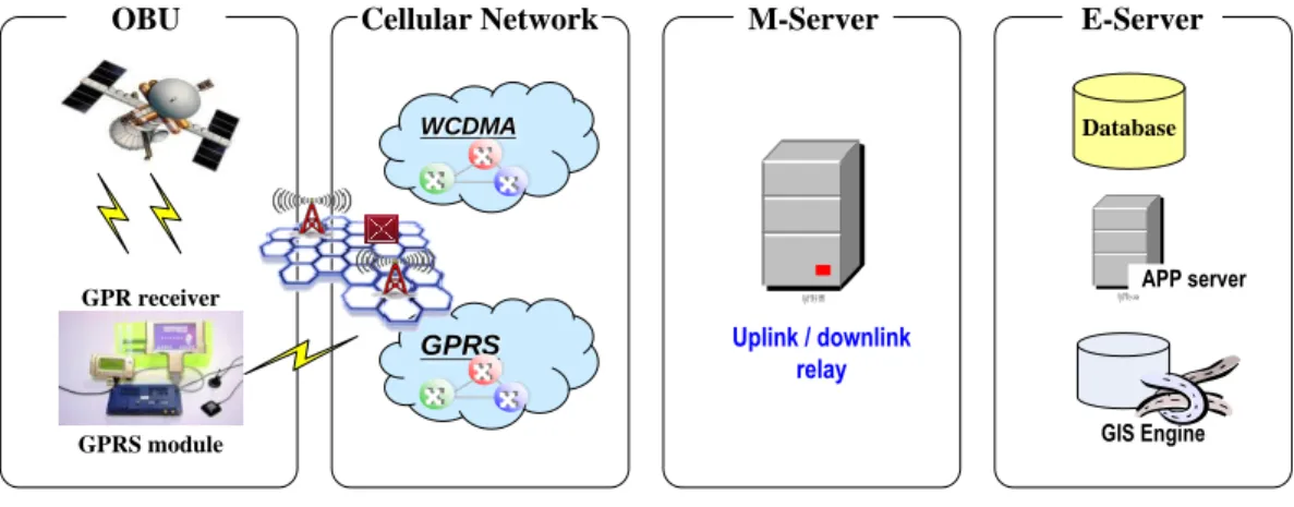
As shown in Figure 1, the system architecture of the LBS system includes: OBU, communication system (cellular network), backend systems (M-Server and E-Server). OBU, a small computer system installed on the vehicle, has computing, positioning, communication and human interface modules. OBU locates the vehicle through receiving GPS satellites signal by positioning module, sends and receives the messages to and from the backend system through the communication module, and interacts with user via the human interface module. Some other tools such as cell or gyro positioning technologies can be the assisted positioning tool when the GPS signal is not available. The communication system is the link between OBU and backend system, which can be any wireless communication mechanism, such as GSM/GPRS/UMTS cellular network, 802.11 wireless network, etc. GPRS cellular network is the most popular communication system in commercialized system, so far. The backend system consists of two parts: M-server and E-server. M-server is responsible for transmitting bi-direction messages and serves as a buffer of uplink and downlink packets between OBUs and backend system over the mobile network. E-Server, consisting of GIS engine, database and application server, is implemented according to the business rules in LBS applications and responsible for the information processes of all the business workflow.
11
OBU Cellular Network M-Server E-Server
GPRS module GPR receiver GPRS WCDMA GIS Engine 伺服器 Uplink / downlink relay Database 伺服器APP server
Figure 1 Components of LBS application
LBS-based applications accomplish the business processes by exchanging information between OBUs and the backend systems. The information is transmitted by the uplink packets (OBUs send to backend) and downlink packets (backend sends to OBUs) over the mobile network. Such interactions among OBUs and the backend system are the basis of the commercial fleet management system. With regarding to the fleet management system as an example, OBU communicates and exchanges information with the dispatching center through the mobile network, which reports the position, direction, speed, and status of the vehicle according to the predefined rules. Dispatching center dispatches and manages the fleet by sending command to the OBUs according to business requirements and the real time positions and status of the fleet.
Taxi dispatching system (TDS), one of the most complicated applications in LBS applications, consists of several participants: customers (passengers), taxi drivers, operators and administrators. OBU automatically registers to the backend system when it is switched on, and turns into „available‟ state. Taxi drivers can change the state of the taxi or interact with the backend system by pressing the
buttons on OBU. There are several buttons designed for the driver to interact with the backend system and operator, including: state changes (available/occupied/ scheduled), polling reply (Y/N/minutes), emergency and message request. Customer requests a taxi via telephone call or Internet web site, operators key-in the requirements and feature of customer and TDS automatically searches the available taxi candidates nearby the location of customer, probing the candidates that fit in with the requirements. The dispatched (received final dispatch message) taxi driver can then response the probing message from TDS, and move on to the corresponding customer‟s location, where administrators are responsible for fleet dispatching, system monitoring, event and exception handling. The OBU automatically interacts with the backend system via uplink packets through the M-server over GPRS cellular network, reporting the status and position of the taxi.
The backend system keeps the latest statuses and positions of all the taxis by collecting all the uplink packets of OBUs. In TDS, there are three kinds of uplink report packet (referred as URP): periodically report (in fixed time interval), cross boundary report (on taxi driving through the geographical boundary), and event report (on status changing or event occurring). By decoding these uplink rules, spatial mobile network information can be derived from communication raw data in LBS-based applications.
13
3.2 Traffic information derived from LBS
The model proposed in this thesis utilizes the raw data of LBS-based application, regards the vehicles in the LBS-based application as the traffic probing vehicle. It is cost effective comparing to the traditional vehicle-based method. Meanwhile, the size of LBS fleet has the temporal and spatial coverage advantages. Traffic information can be dynamically gathered in the LBS fleet operation area 24 hours per day in real time.
The vehicles of LBS are regarded as the traffic status probing vehicles of the urban network. A vehicle in the LBS application is equipped with an OBU, which has GPS (Global Positioning System) positioning module and wireless data communication module such as GPRS/UMTS. OBU collects vehicle position, traveling direction, and speed from the GPS module and uplinks the vehicle status to the backend system through communication module.
)
,
,
,
(
)
,
,
,
,
,
(
X
Y
t
V
D
S
TIS
L
T
V
D
U
p
Gis i s (3.1)Each uplink packet (Up) representing the current position and traveling status of that vehicle, as shown in equation (3.1), is sent from the probing vehicle to the backend system. The information in Up includes: position coordinate(X, Y), traveling speed (V), direction (D), timestamp (t) and status (S). By combining with GIS, coordinate of a vehicle can be transformed to nearest address by interpolating the GPS position with road network database [11]. Thus traffic information can be gathered by transforming the uplink packet into traffic
information spot (TIS) of the link where the vehicle located (Li). A TIS (Li,Ts,V,D) is a sample of traffic information at two dimensions : spatial dimension (Li) and temporal dimension (Ts), which represents the traveling speed (V) and direction (D) of the link at these two spatiotemporal indices. Then, the real time traffic information of the urban network can be derived from LBS by aggregating all the collected TISs at the current time interval, for example, quarter or half an hour.
15
Chapter 4
Spatiotemporal Bottleneck Mining Models
The architecture of spatiotemporal bottleneck mining model (STBM) proposed in this thesis is shown in Figure 2. First of all, the raw data of LBS is used to extract the meaningful traffic congestion patterns, and then our three heuristics are applied to give reasonable interpretation for the congestion patterns. We describe three kinds of heuristics to interpret extracted traffic congestion patterns as follows: (1) congestion-propagate heuristic (CPH): if a bottleneck congests, as a consequent,it may result in more congestions to other objects, (2) congestion-converge heuristic (CCH): if a bottleneck congests, it must be caused by some other prior congested objects, (3) congestion-drop heuristic (CDH): if the congested status of an object decreases dramatically or even disappears afterwards, then it is treated as a bottleneck.
The whole STBM model is divided into three phases: traffic information generation, traffic congestion patterns and spatiotemporal bottleneck mining, as illustrated in Figure 2. Traffic information database is generated from Location-Based Service (LBS) applications and Geographical Information System (GIS) urban network database in first phase. In Phase II, the traffic congestion patterns are extracted from the traffic information database obtained from Phase I, and there are two kinds of traffic congestion patterns: congestion consequent patterns (CCP), congestion drop downstream patterns (CDDP). Finally, the three
heuristics are used to interpret the traffic congestion patterns which will be used to discover the spatiotemporal bottlenecks in Phase III. The detailed discussion about the whole model is described in the following sections.
GIS LBS Traffic Information Generation Phase I Traffic Congestion Patterns Recognition
Phase II Phase III
Congestion-Drop Heuristic Congestion-Converge Heutistic Congestion-Propagation Heuristic Spatiotemporal Bottleneck Figure 2 Architecture of STBM
4.1 Phase I: Traffic Information Generation
Traffic information generation is the first phase in STBM. Raw data is collected from LBS-based applications (discussed in 3.1) and transformed into traffic information by combining the road network database in the GIS engine. Traffic network is composed of a set of connected network objects, where an object is either a link or an intersection. As shown in Figure 3, the white real line means links, and the red spot means the intersections in the network.
17
N
Figure 3 An example of traffic network which is composed of a set of links and intersections
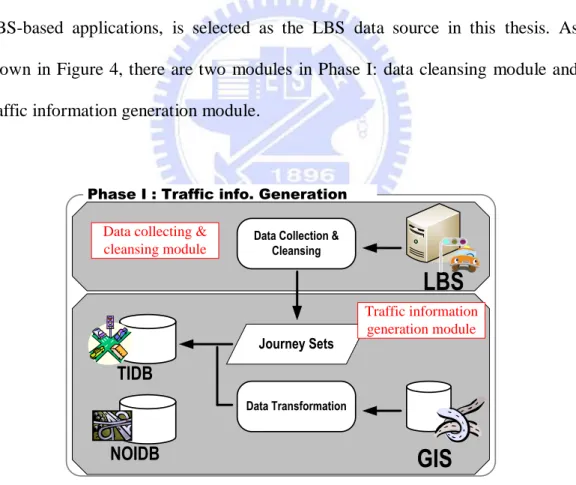
Taxi dispatching system (TDS) [7], which is one of the most complicated LBS-based applications, is selected as the LBS data source in this thesis. As shown in Figure 4, there are two modules in Phase I: data cleansing module and traffic information generation module.
Phase I : Traffic info. Generation
GIS
LBS
Journey Sets
Data Collection & Cleansing
Data Transformation
TIDB
Traffic information generation module Data collecting &
cleansing module
NOIDB
In data collection and cleansing module, a batch process collects raw data from TDS system periodically (e.g., every day), and also collects the communication logs between the front-end devices (i.e., OBU) in the vehicles (i.e., taxis here) and backend system in the TDS system. The extracted vehicle journey information of each vehicle can then be transformed into vehicle journeys information.
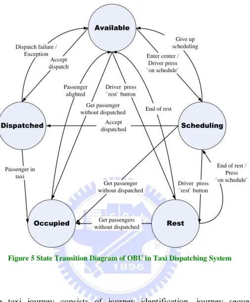
Traffic information generation module extracts „meaningful‟ taxi journey information by grouping and sorting the uplink records of each taxi and transforms the data into traffic spots by combining traffic network information from GIS. Thus, a journey consists of a set of meaningful continuous traffic spots reported by the same vehicle starting from origination to the destination. Here “meaningful” journey means the taxi is in the „dispatched‟ or „occupied‟ states. In other words, the taxi must be in „driving‟ state, and a journey is a set of continuous traffic spots of the same vehicle. The state transition diagram of OBU in TDS is shown in Figure 5.
19 Available Dispatched Scheduling Occupied Rest Dispatch failure / Exception Accept dispatch Passenger alighted Get passenger without dispatched Driver press `rest` button End of rest Accept dispatched Get passenger without dispatched Get passengers without dispatched Driver press `rest` button End of rest / Press `on schedule` Passenger in taxi Enter center / Driver press `on schedule` Give up scheduling
Figure 5 State Transition Diagram of OBU in Taxi Dispatching System
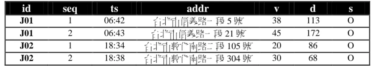
The taxi journey consists of journey identification, journey sequence, timestamp, address, speed, vehicle direction, and state of a taxi. It can be formulated as a vector <id, seq, ts, addr, v, d, s>, where the information of address, speed, and direction provides good data sources for mining traffic status of urban network. Journey id and sequence provide information for OD (origination and destination) analysis, where seq=1 indicates the origination and the last seq number of the same journey id represents the journey destination. Table 1 gives an example to illustrate the taxi journey.
Table 1 An example of taxi journey reported from probing vehicles id seq ts addr v d s J01 1 06:42 台北市信義路一段 5 號 38 113 O J01 2 06:43 台北市信義路一段 21 號 45 172 O J02 1 18:34 台北市敦化南路二段 105 號 20 86 O J02 2 18:38 台北市敦化南路一段 304 號 30 68 O
After data collecting process, noise data (e.g., invalid values of speed, direction, or GPS state) need to be removed from the collection date, so we classify the useless data into three categories which are listed as follows:
1. Missing Values
There are some links of which probing vehicles do not record the traffic status information may due to GPRS communication or GPS errors. GPS errors might occur when a probing vehicle passes under an infrastructure such as tunnel or the vicinity of elevated structures (the so called urban canon). GPRS communication might be done in similar way or any unknown events to cause missing values.
2. Useless Data
If a probing vehicle`s speed is 0 for a long time and its status is ”driving”, we assume the vehicle is stopping in the ranking station and waiting for servicing because the LBS based probing vehicles are commercial taxi fleets and have “taxi behaviors” on their operating. Therefore in the content of URP, if a probing vehicle`s speed is 0 in the same position for a long time, this record is thought as a useless data.
21
3. Redundant
Some reports of URP show the same messages from the same vehicle. This is because there may be several events occurred simultaneously, such as periodically report event after the cross boundary event. So, the reports of message which are counted twice need to be pruned.
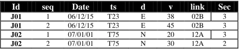
Data cleansing module is used to filter out the useless or incomplete data described above to facilitate the further analysis. Traffic information generation module then extracts useful taxi journey information and transforms it into traffic information database (TIDB) which contains the useful and meaningful traffic journey information by combining traffic network information from GIS. This can be done by transforming the report coordinates of each vehicle report point to the real traffic network address helped by the coordinate to address transforming function in GIS engine [10]. Each record in TIDB includes eight fields, journey identification, journey sequence, date, timeslot, dir, speed, link identification, and the section number of link, it can be formulated as a vector <id, seq, date, ts, d, v, link, sec>, where the timeslot is normalized, e.g., T1 to T96 which splits every 15 minutes into a timeslot, the link indicates the corresponding link identification, and sec means the section number of the location. Table 2 gives an example of TIDB.
Table 2 An example of TIDB
Id seq Date ts d v link Sec
J01 1 06/12/15 T23 E 38 02B 3
J01 2 06/12/15 T23 E 45 02B 3
J02 1 07/01/01 T75 N 20 12A 3
J02 2 07/01/01 T75 N 30 12A 2
The traffic information of the traffic network objects can be obtained by an aggregation on the TIDB generated in the first phase. Each record in TIDB (i.e., a traffic information spot (TIS)) represents a piece of traffic information about where, when and how the vehicle is in the spatial and temporal condition.
Furthermore, we also construct network objects information database (NOIDB) which records the traffic status about all objects in the traffic network in each timeslot, there are six attributes in NOIDB: link, sec, dir, ts, limit, speed; limit indicates the speed limitation of this link, and speed are average driving speed calculated from TIDB of the corresponding link, sec, dir, and timeslot, and Table 3 gives an example of NOIDB.
Table 3 An example of NOIDB
link sec dir ts limit speed
01A 1 N T1 60 30
01A 1 S T1 60 55
10B 1 E T3 50 36
23
4.2 Phase II: Traffic Congestion Patterns Mining
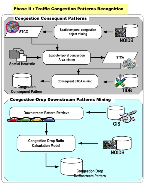
Figure 6 represents the architecture of Phase II in STBM, and there are two modules for discovering the congestion patterns which are congestion consequent patterns (CCP) mining and congestion drop downstream patterns (CDDP) mining from the traffic information derived from Phase I.
Phase II : Traffic Congestion Patterns Recognition
STCA STCO Spatiotemporal congestion object mining
TIDB
Spatial Heuristic
Spatiotemporal congestion Area mining
Congestion Consequent Patterns
NOIDB
Congestion-Drop Downstream Patterns Mining
Downstream Pattern Retrieve
GIS
Congestion Drop Ratio Calculation Model
Congestion Drop Downstream Pattern
NOIDB
Consequent STCA mining Congestion
Consequent Pattern
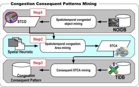
4.2.1 Congestion Consequent Patterns Mining
Figure 7 represents the architecture of congestion sequential patterns mining module, and including three processes: (1) spatiotemporal congested object (STCO) mining, (2) spatiotemporal heuristic clustering Algorithm (SHC) to cluster a set of STCOs into a spatiotemporal congestion area (STCA), and (3) discovering the consequent STCAs for each STCA as the congestion consequent patterns.
Congestion Consequent Patterns Mining
STCA STCO Spatiotemporal congested object mining
TIDB
Spatial Heuristic
Spatiotemporal congestion Area mining
Consequent STCA mining Congestion Consequent Pattern NOIDB Step1 Step2 Step3
Figure 7 The architecture of congestion consequent patterns mining
As we know, it is very difficult to represent the traffic status of each network object because of the different road categories and different time. For example, traffic status of average speed 35 km/hr on the workday peak hours for street may indicate that the traffic status on the street is „free‟, but on the expressway the same condition indicates the „congestion‟ state.
25
As mentioned above, a normalized formulation about the traffic status of a network object must be given. Traffic index factor (θ) is defined in order to normalize the traffic status, as shown in equation (4.1), where i is for the object index andVi, Si represents the average speed and speed limit of the object i
respectively due to the different road categories. The greater value of θ means the more serious congestion level of the object. θ equals one means the object is in a serious congestion status and θ near around zero means the object is in a free flow status. The traffic status of a network object Oi is formulated as a four elements vector Oi=<Sid, Tid, d, θ>, elements in the vector represent spatial id, temporal id,
direction, and traffic index factor.
Si
Vi
-1
(4.1) By normalizing the traffic index factor (θ) of all the objects, we classify the traffic status of a network object by five classes (i.e., 1~5), where 1 indicates free flow state, and 5 indicates strongly congested state. So, the network object vector can be modified as Oi=<Sid, Tid, d, θ, c>, where c is the traffic status class (1~5).By aggregating the TIS, each network object in the traffic network has its own θ
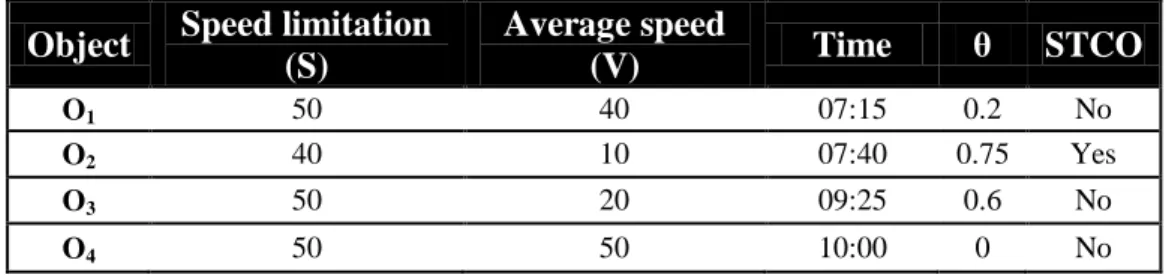
i, a threshold of θ called Congestion-Bound (CB) is used to determine whether an object is in congested status or not, if θ of network object is bigger than CB then the object is thought as a spatiotemporal congested object (STCO). An example of network object attribute and STCO determination is listed in Table 4, and CB is set to 0.75. In this example, only network object O
2 is justified as STCO because its θ value is greater than or equal to the threshold (0.75).
Table 4 An example of network object status, CB=0.75
Object Speed limitation (S) Average speed (V) Time θ STCO O1 50 40 07:15 0.2 No O2 40 10 07:40 0.75 Yes O3 50 20 09:25 0.6 No O4 50 50 10:00 0 No
All traffic spots by spatial and temporal domain can be aggregated to represent the traffic status of urban network, where spatial domain groups the traffic spots by network objects, and temporal domain groups the traffic spots by time periods, for example, 15 minutes. Therefore it is easy to snapshoot the traffic status of the urban network by spatiotemporal aggregating all the traffic spots, and the traffic status of urban network can be easily represented using the traffic status snapshots. For example, the traffic status of urban network in morning peak hour (7~9 AM) includes eight 15-minutes network snapshots.
Since the congested objects are found, we have to decide which congested objects might be the bottleneck. Only mining the information of objects (a link or an intersection) to find the relation between each other is not reliable due to the lower confidence. Our idea is to raise the confidence by clustering the STCOs into clusters so that the reliability will be increased. The clustering Algorithm we proposed called Spatiotemporal Heuristic Clustering Algorithm (SHC) is proposed.
27
Spatial Heuristic Clustering Algorithm (SHC)
After STCOs are found, the second process in this phase is spatiotemporal congestion area (STCA) clustering, which clusters the STCOs in urban network into several clusters. We develop a Spatiotemporal Heuristic Clustering (SHC) Algorithm which is a three-dimensional clustering algorithm comparing to traditional two-dimensional clustering algorithm such as K-means, ISODATA. The SHC algorithm (Algorithm 1) clusters the STCOs by the spatiotemporal clustering consideration.
Unlike the traditional two-dimension spatial clustering algorithm, the SHC algorithm is a three-dimension algorithm with additional temporal dimension. Every round of the SHC Algorithm deals with a network snapshot, and clusters all the STCOs on that snapshot by the temporal dimension.
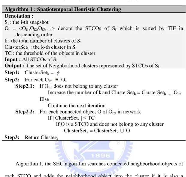
Algorithm 1 Spatiotemporal Heuristic Clustering Algorithm
Algorithm 1 : Spatiotemporal Heuristic Clustering Denotation :
Si : the i-th snapshot
Oi = <Oi1,Oi2,Oi3,…> denote the STCOs of Si which is sorted by TIF in descending order
k: the total number of clusters of Si ClusterSetk : the k-th cluster in Si
TC : the threshold of the objects in cluster Input : All STCOs of Si
Output : The set of Neighborhood clusters represented by STCOs of Si Step1: ClusterSetk =
Step2: For each Oim Oi
Step2.1: If Oim does not belong to any cluster
Increase the number of kand ClusterSetk = ClusterSetk ∪ Oim Else
Continue the next iteration
Step2.2: For each connected object O of Oim in network If | ClusterSetk | ≤ TC
If O is a STCO and does not belong to any cluster ClusterSetk = ClusterSetk ∪ O
Step3: Return Clusterk
Algorithm 1, the SHC algorithm searches connected neighborhood objects of each STCO and adds the neighborhood object into the cluster if it is also a congested object (STCO) and does not belong to any cluster. Besides, we assume the total number of objects in cluster is less than TC, which is the length limitation of cluster, and each cluster contains no more than TC congested objects. Until all STCOs in snapshot belong to some cluster, SHC is finished. Finally, all clusters returned are the spatiotemporal congestion areas (STCA) of each snapshot.
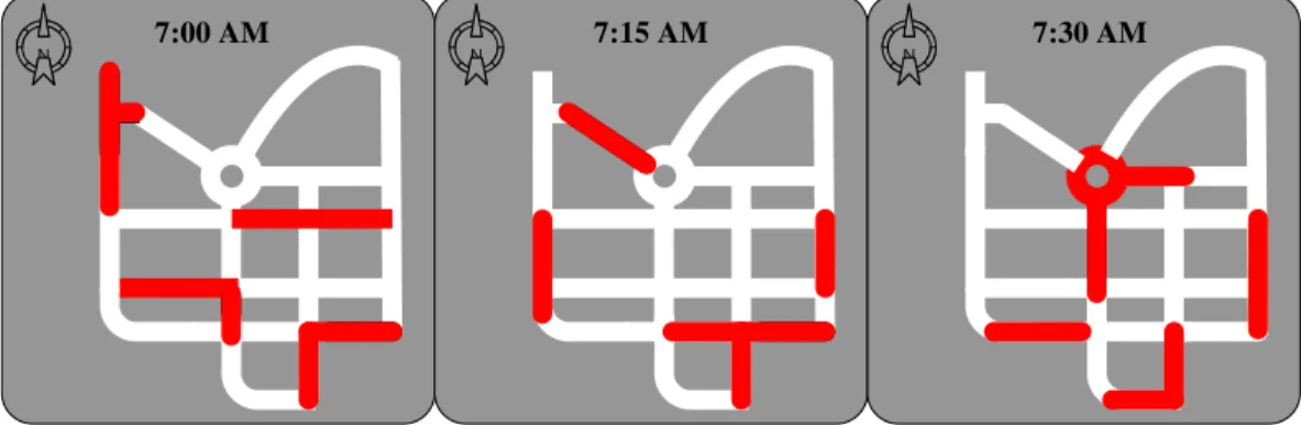
Figure 8 gives an example of three snapshots of the same network, which are 7:00AM, 7:15AM, 7:30AM respectively. Each connected red part indicates a
29
STCA which is composed of at least STCO, and we can find each snapshot has four STCAs.
N 7:00 AM N 7:15 AM N 7:30 AM
Figure 8 An example of three snapshots of the same traffic network.
The final process of congestion sequential patterns mining module we proposed here is to discover the relations between STCAs (i.e., Consequent STCA Mining Algorithm (CSM)) by utilizing the TIDB derived from Phase I and the congestion area produced by SHC algorithm.
Consequent STCA Mining Algorithm (CSM)
After the connected congested objects of each snapshot are clustered as a set of STCAs, the next step is to find the consequent relationship between congestion areas by an algorithm so called Consequent STCA Mining (CSM) Algorithm which is described in the following.
Algorithm 2 Consequent STCA Mining Algorithm
Algorithm 2 : Consequent STCA Mining (CSM) Denotation:
S=<So,S1,S2,…> denotes all snapshots ordered by timestamp Ai=<Ai1,Ai2,Ai3> denote all STCAs of Si
T: the temporal limitation of consequent STCAs DOR-Bound: threshold of DOR
Consequent Pair (Am,An) : pair (Am,An) , where the time interval between Am and An ≤ T and the DOR of the pair ≥ DOR-Bound
PairSet: all pairs
ResultSet : the set of all consequent pairs Input: STCAs on all snapshots
Output: ResultSet
Step1: PairSet = and ResultSet = Step2: For each Aik of Si
For each A in Si+1, Si+2,…, Si+T
Construct P=(Aik,A) and PairSet = PairSet ∪ P Step3: For each P=(Am,An) in PairSet
Step3.1: Calculate DOR(P)
Step3.2: If DOR(P) ≥ DOR-Bound ResultSet = ResultSet ∪ P Step4: Return ResultSet
CSM aims to find out all consequent STCAs of each STCA; therefore, we find pair P=(Am, An) which denotes there might be a consequent relation between Am and An. Moreover Consequent Pair (CP) denotes the pair P=(Am, An) and there is a consequent relation between Am and An indeed which means An is the c of Am and also the difference of timestamp of Am and timestamp of An should be less than T. In other words, if Am is in congestion, An will be in congestion consequently. The TIDB derived from Phase I, in detail, records the information about the journey: the journey identity, origin, destination, the position with the time it traveled. These particular records can help us to identify which An is really a consequent of Am.
31
The Demand overlapped ratio (DOR) of P=(Am, An) is defined in equation (4.2), which indicates how much proportion of journeys of An are coming from Am, and Om,n means the number of the same journeys in Am and An; Jn means the total journey number of An. By definition, the value of ranges from 0 to 1, when =0 means there is no journey from Am to An and also implies P is not a CP; otherwise, if =1, it means the all journeys in An are coming from Am and they have a very strong consequent relationship and P is a CP. Therefore the larger then the stronger relationship of P will be, and if larger than DOR-Bound, which is the threshold of , then P is a CP.
n n m
J
O
,
(4.2) There gives an example in Table 5 to illustrate the demand overlapped ratio, and DOR-Bound is set to 0.6, after DOR being calculated, the P1 and P3 are considered as Congestion Consequent Pairs (CCP).Table 5 An example of Demand Overlapped Ratio with DOR-Bound=0.6
pair (Am,An) Om,n Jn DOR Consequent Pair
P1=(A1,A2) 40 60 0.667 Yes
P2=(A1,A3) 10 40 0.25 No
P3=(A3,A5) 60 80 0.75 Yes
4.2.2 Congestion-Drop Downstream Patterns Mining
Congestion-Drop Downstream Patterns Mining
Downstream Pattern Retrieve
GIS
Congestion Drop Ratio Calculation Model
Congestion Drop Downstream Pattern
NOIDB
Figure 9 The architecture of Congestion-Drop Downstream Patterns mining
The Congestion-Drop Downstream Patterns (CDDP) Mining module is shown in Figure 9. The traffic stream has some directions, and then each object with direction in network has its upstream and downstream objects. Figure 4.9 gives an example to illustrate the traffic stream. Each number represents the identity of every network object; if the direction of object4 is “east” then its upstream objects are: (object1, south), (object3, east), and (object6, north) and its downstream objects are: (object2, north), (object5, east), and (object7, south). The GIS engine can provide the geographical features of traffic network and the geographical relationship between each pair of network objects, which can be used to construct the downstream patterns.
33
Definition: Downstream Patterns (DP)
Each object in traffic network has its own downstream objects, the Downstream Pattern (DP) can be defined as follows:
DS (Oi) = {Oi1, Oi2, … , Oik} : which is a set of objects denoting the
downstream objects of Oi, where k is the total number of downstream objects of Oi.
DP(Oi) = (Oi, DS(Oi), k) : each DP is defined as a triple indicates the
network object Oi, its downstream objects as a set, and the number of its downstream objects.
N
1
2
3
4
5
6
7
Figure 10 An example of traffic stream in network
Take Figure 10 as an example, we can get seven DPs from the network, e.g., DP (Obiect4) = (Object4, {Object2, Obect5, Object7}, 3). After DPs are constructed, we utilize the NOIDB derived from Phase I to find out the Congestion-Drop Downstream Patterns (CDDP) from DPs based on Congestion-Drop Heuristic (CDH). The idea of CDH is:” if the congested status
of an object decreases dramatically or even disappear afterwards, then it is treated as a bottleneck”; therefore, we can use the traffic index factor θ to extract CDDP from DPs, since the serious congested status indicates the higher θ and the free traffic indicates the lower θ.
For each DP= (Oi, DS(Oi), k) and DS (Oi) = {Oi1, Oi2, … , Oik}, we can calculate the difference of θ between Oi and its downstream objects DS(Oi) called Congestion Drop Ratio (CDR) χ , which is defined as equation (4.4), and θi is θ of Oi and θi1 to θik are θ of Oi`s downstream objects and k is the total number of downstream objects, so χ is the congestion difference between Oi and its
downstream objects.
k
O
k j ij i i
1)
)
DP(
(
(4.4)The value of χ is less than or equal to 1 and might be negative, when χ is close to 1 means the average θ of downstream objects is almost equal to 0 and θ of Oi is very close to 1 then DP(Oi) is a CDDP according to CDH. Otherwise, if χ is smaller than 0 means the θ of Oi is smaller than the average θ of its downstream
objects and its physical meaning indicates the congested status is more serious in downstream than in Oi, then DP(Oi) disobeys the CDH and it is not a CDDP. Therefore if χ of DP is bigger than CD-bound, which is threshold of χ, and we can conclude this DP is also a CDDP.
35
4.3 Phase III: Spatiotemporal Bottleneck Mining
The two congestion patterns mining from Phase II are: (1) congestion consequent pair (CCP): (Am, An) which means if the STCA Am congests, An will congest consequently. Am is the antecedent of the pair and Aj is the consequent of the pair, (2) congestion drop downstream pattern (CDDP): (Oi, DS(Oi), k), DS(Oi) means the downstream objects of Oi and k is the number of DS(Oi). In this phase, we use two heuristics to verify the CCP we discovered from Phase II, and use the congestion confidence (CC) τ to verify the CDDP and to find out all the three kinds of bottlenecks.
4.3.1 Congestion-Propagation Heuristic
The idea of congestion-propagation heuristic (CPH) is:” if a bottleneck congests, as a consequence, it may result in more congestions to other objects”, therefore we know this heuristic is based on congestion consequent pairs discovered from Phase II. According to congestion-propagation heuristic, the bottlenecks may occur in the antecedent of consequent pairs.
We define root-cause STCA (RC-STCA) as STCA which may imply more STCAs in consequent pairs, and means RC-STCA appears in the antecedent part of all consequent pairs is more than CPH-Bound times, which is a threshold of CPH. By definition of congestion-propagation heuristic, the bottlenecks may exist
in RC-STCA; therefore, the bottleneck mining can only be limited to RC-STCAs. All STCOs in RC-STCAs are thought as the bottleneck candidates.
i i i
all
c
(4.3) The bottleneck must be in congested status more often or otherwise it is not a bottleneck; therefore, the congestion confidence τ is used to extract the real bottleneck from the bottleneck candidates. The definition of τ is given in equation (4.3), where ci means the congested days in the experiment and alli means the total experiment days. The value of τ ranges from 0 to 1 and when τ= 1 means the object is always congested; otherwise when τ= 0 indicates the object is always free. Therefore, if the congestion confidence of bottleneck candidate BC is larger than CC-Bound, which is the threshold of τ, we may conclude it is an STB.4.3.2 Congestion-Converge Heuristic
The idea of congestion-converge heuristic (CCH) is:” if a bottleneck congests, it must be caused by some other prior congested objects”; therefore, we know this heuristic is also based on congestion consequent pairs, and the bottlenecks may occur in the consequence of consequent pairs. The root-cause STCA (RC-STCA) is defined as the STCA, which appeared in the consequent part of all consequent pairs, is more than CCH-Bound times, which is a threshold of CCH. As shown in Section 4.3.1, the bottleneck mining can only be limited to RC-STCAs. All STCOs in RC-STCAs are thought as the bottleneck candidates
37
and we use congestion confidence τ (defined in equation (4.3)) to finally determine whether it is an STB or not. If τ of a bottleneck candidate is bigger than CC-Bound, we may conclude the bottleneck candidate is an STB.
4.3.3 Congestion-Confidence to Verify CDDP
Since congestion drop downstream pattern (CDDP) =(Oi, DS(Oi), k), DS(Oi) are found in Phase II, the Oi is thought as a bottleneck candidate based-on congestion drop heuristic (CDH); therefore, we have to check the congestion confidence τ of Oi to decide if it is a spatiotemporal bottleneck or not. If τ of a bottleneck candidate is bigger than CC-Bound, we may conclude the bottleneck candidate is an STB.
38
Chapter 5
Experiments
The STBM prototype model was implemented based on a real time LBS-based application: taxi dispatch system (TDS) [2]. The TDS is an online 724 system operated in Taipei urban area, and the current fleet size is about 500 taxis, where the OBU reports its current status periodically (30 sec) or when some events occur. The types of event include spatial trigger event, dispatch/response event, customer on/off taxi events, etc. Currently TDS raw data could be half a million uplink reports per day, which becomes a good data source for this prototype model. In the data collecting and cleansing module, the OBU raw data has been collected and transformed to TISs in a period of 5 minutes in order to catch the real time traffic information and only the traffic information in „dispatch‟ or „occupied‟ state of OBU is extracted.
Historical traffic information consists of journey sets, which can be obtained from the raw data by combining the GIS road network. For example, „dispatch‟ state journey starts from the dispatch location to the customer‟s location, and „occupied‟ state journey starts from the customer‟s location to customer‟s destination.
39
Figure 11 Main roads in Taipei urban network
As shown in Figure 11, the target area of this prototype system focused on the urban network in Taipei city; each arterial in the network may have at least one link. The predefined link attributes including category, length, direction, speed limit, average signal delays and geographical coordinates vectors with default values are given by domain expert to facilitate STB discovering. In the congestion area mining phase (Phase II), traffic index factor θ is classified by aggregating the TISs at temporal and spatial dimensions and normalized by category and speed limit attributes. For example, if the traffic index factor is very close to 0 it means the link is in free flow state and the traveling speed is near around the speed limit; on the other hand, if traffic index factor is close to 1 it represents that the link is in extremely congestion status.
In the experiment, raw data was collected during 2006/02~2007/03; the data in the first eleven months is for training the STBM model and the remaining is for
testing. The traffic index factor (θ) for workday and weekend are summarized as depicted in Figure 12, where each plot in Y-axis means a 15 minutes time slot. In Figure 12, it can be easily seen that there are two peaks in the curve of workday, which verify the common experience of on-duty and off-duty peak hours. Nevertheless, the curve of weekend does not have the obvious peak due to different patterns on workday and weekend. Therefore, we limit the STB search period on two peak hours of the workday in order to reduce the computing complexity. The average θ of the on-duty peak hour (07:30~09:30) is 0.45, and off-duty peak hour (17:30~19:30) is 0.54.
Figure 12 Traffic index factor (θ) for workday and weekend
The testing data from January to March in 2007 is divided into twelve weeks for testing, and three methods we proposed will be compared to the statistic model, which chooses the top k objects with the highest TIF and highest congestion
41
confidence. The experimental results in workday and weekend are shown in Figure 13 and Figure 14 respectively. Figure 13 shows the experiment of workday accuracy between three heuristics in STBM and statistic model, the accuracy of four methods are all around 75%; moreover, CPH and CCH are more stable than other two methods (CDH, statistic) and also have higher accuracy. Though the average accuracy (see Table 6) of statistic model is as good as STBM but it is not steady, the accuracy in some weeks are not higher as we expected.
Figure 13 Three heuristics of STBM compare to statistic model in workday
Table 6 The average experiment accuracy.
CCH CPH CDH Statistic
Workday 0.795982 0.776282 0.7469 0.759009
Weekend 0.726056 0.618511 0.714767 0.55
The experimental results as shown in Figure 14, the accuracy in weekend is much unstable than the experiment results in workday and the workday results are better than weekend because the weekend traffic does not have the general traffic
pattern, like the workday traffic which always has the two clear patterns: (1) on-duty pattern which from home to company in the morning and (2) off-duty pattern which from company to home in the evening, so the accuracy distribution is much dispersed. But the average accuracy of STBM is still better than statistic result as shown in Table 5.1.
Figure 14 Three methods of STBM compare to traditional statistic model in weekend
In Figure 15, the link on the map is the main roads of urban network, and the right-down side is the urban center and there are three arrows mined by CPH located on Taipei urban network: white means the on-duty bottlenecks on 7:30 to 9:30 in the morning; blue means the off-duty bottlenecks on 5:30 to 7:30 in the evening; and yellow means the bottlenecks both in the morning and evening. The four edges of the map is the suburban, and we can see the on-duty bottlenecks is from the suburban into the urban center which is just like the traffic pattern when go to the work; furthermore the off-duty bottlenecks is just from the urban city
43
center to suburban which also means the traffic pattern going home. In Figure 15, we can see that the reliability and accuracy of STBM are quite high.
44
Chapter 6
Conclusions and Future Works
Finding out bottlenecks in traffic network is one of the major tasks in ATMS in order to take some actions for improving global network performance. The STBM model, we proposed in this thesis, consists of three phases (traffic information generation, traffic congestion patterns and spatiotemporal bottleneck mining) for discovering the spatiotemporal bottlenecks in urban network. It utilizes the raw data collected from LBS-based applications (which has the advantages in term of cost and coverage comparing to traditional sensor based surveillance system) and the road network information from GIS for discovering the bottlenecks.
Three heuristics for finding out bottlenecks are proposed to find the total solution to traffic network bottleneck, and experimental results showed that the average accuracy in workday using three heuristic-modules are higher than 76% and better than statistic model. Moreover, the average accuracy in weekend is little lower than workday may due to the clear traffic patterns in workday i.e., on-duty pattern in the morning and off-duty pattern in the evening. The basic idea of CPH and CCH is utilizing the consequent rules to gain the bottleneck; therefore the accuracy in weekend is a little bit lower than workday.
45
In the near future, the STBM model will be enhanced as a real time bottleneck detection and prediction system, which integrates the historical traffic patterns and real-time traffic information to predict the bottlenecks. And further traffic assignment suggestions will be provided by combining the domain knowledge of traffic assignment experts with the enhanced STBM model.
46
Reference
[1] E. Chung, “Classification of Traffic Pattern,” Proc. 11th World Congress on ITS, 2003.
[2] E. Chung, et al., “Travel Time Prediction: Issues and Benefits,” Proc. of the 10th World Conference on Transport Research, 2003.
[3] Hsiao-Han Chen, Wei-Hsun Lee and Shian-Shyong Tseng “A Spatiotemporal Traffic Bottlenecks Mining Model for Discovering Bottlenecks in Urban Network,” 14th World Congress on ITS 2007, Beijing, China.
[4] T. Kawahara, S. Kamijo and M. Sakauchi, “Travel time measuring by using vehicle sequence matching between adjacent intersections,” Proc. IEEE International Conf. on Intelligent Transportation Systems, 2005, pp. 712-717.
[5] B. S. Kerner and DaimlerChrysler AG, ”Control of Spatiotemporal Congested Traffic Patterns at Highway Bottlenecks,” Proc. of the 8th International IEEE Conference on ITS, 2005.
[6] B. S. Kerner, C. Demir, R. G. Herrtwich, S. L Klenov, H. Rehborn, M. Aleksi, A. Haug and G. DaimlerChrysler A, “Traffic State Detection with Floating Car Data in Road Networks,” Proc. of the 8th International IEEE Conference on ITS, 2005.
47
[7] H. Y. Liu, C. H. Wang, V. S. Shieh and B. S. Jeng, “An intelligent taxi dispatching management system,” Proc. of Cross Strait Conference on ITS, 2004, pp. 111-117.
[8] W.-H. Lee, B.-S. Jeng, S.-S. Tseng and C.-H. Wang, “Electronic Toll Collection Based on Vehical-Positioning System Techniques,” Proc. 2004 IEEE International Conf. on Networking Sensing and Control, pp. 643-648. [9] H.-E. Lin and R. Zito, “A Review of Travel-Time Prediction in Transport and Logistics,” Proc. of the Eastern Asia Society for Transportation Studies, Vol. 5, pp. 1433 - 1448, 2005.
[10] Sheng-Han Tsai, Wei-Hsun Lee and Shian-Shyong Tseng, “A spatiotemporal traffic patterns mining on LBS-based application,” TAAI 2005
[11] C. W. Wang, C. C. Chiu, S. D. Jeng, S. R. Hsiao, L. G. Wei, C. H. Chao, and C. H. Hwang. “A Geocoding Application on GIS Using Address Data: Case Study of Taiwan Address Database,” Proc. of TGIS 2003 Annual Conf., Taipei, Taiwan, pp. 25-26.
[12] J.-S. Yang “Travel Time Prediction Using the GPS Test Vehicle and Kalman Filtering Techniques,” Proc. of the 2005 American Control Conference, pp. 2128-2133, June 8 - 10, 2005.
[13] H. S. Zhang, Yi Zhang, Z. H. Li and D. C. Hu, “Spatial-Temporal Traffic Data Analysis Based on Global Data Management Using MAS,” IEEE Trans. on ITS, Vol. 5, No. 4, December 2004, pp. 267-275.