以全域最佳化方法求解DNA序列之共同區間定址問題(II)

行政院國家科學委員會專題研究計畫 期中進度報告

以全域最佳化方法求解 DNA 序列之共同區間定址問題(2/3)

計畫類別： 個別型計畫

計畫編號： NSC94-2213-E-009-040-

執行期間： 94 年 08 月 01 日至 95 年 07 月 31 日

執行單位： 國立交通大學資訊管理研究所

計畫主持人： 黎漢林

計畫參與人員： 傅昶瑞

報告類型： 精簡報告

報告附件： 出席國際會議研究心得報告及發表論文

處理方式： 本計畫可公開查詢

中 華 民 國 95 年 5 月 22 日

行政院國家科學委員會專題研究計畫期中進度報告

以全域最佳化方法求解 DNA 序列之共同區間定址問題 (2/3)

A Linear Programming Approach for Identifying a Consensus Sequence on

DNA Sequences (2/3)

計畫編號：NSC 94-2213-E-009-040

執行期限：94 年 8 月 1 日至 95 年 7 月 31 日

主持人： 黎漢林 國立交通大學資訊管理研究所

本研究為三年期計畫，目的在於發展全域最佳化技術來解決基因序列共同區間的尋找問 題。在多組基因序列間尋找共同區間的問題，在生物資訊的分析上是相當常見的。部分案例中 這個共同區間還需要包含結構性的限制，mRNA 中 stem-loop motifs 的尋找即為其中一例。

在本計畫中這類問題首先將被轉換成非線性 0-1 的數學模式。該模式經過轉換後可以變成 包含有限個 0-1 變數的線性模式，且可利用分散式計算來快速求解。此方法保證可以找到全域 最佳解，其運算速度也遠優於任何現今被提出的方法。 第一年本計畫將進行該方法的發展及驗證，第二年與第三年針對各種在生物資訊分析方面 可能的應用來延伸開發其應用的作法，且發展自動化的應用程式系統來完成分散運算的能力。 關鍵詞：最佳化、生物資訊、分子生物學、蛋白質鍵結 Abstract

This plan is about to develop a global optimization method in identifying a set of protein binding sites in a set of unaligned DNA fragments. The identification of common sites in multiple sequences is frequently encountered in the analysis of biopolymer sequence data. In several cases there exists various kind of structural constraints in such a problem. An example is the stem-loop motifs in mRNA molecules.

Firstly the problem is formulated as a nonlinear 0-1 optimization model. This model is then converted into a linear 0-1 problem solvable by distributed computation system. The technique is guaranteed to find a global optimum. In additional, the computational speed of this technique is much

In first year we develop this methodology and verify the performance. And in the following two years we will apply this method to various types of practical use. Meanwhile a distributed computation system will developed to enhance the computation.

Keywords: Optimization, Bioinformatics, Molecular biology, Protein binding

1. Introduction

The methods for determining a consensus pattern can be split into two parts. The first part is the model for describing the shared pattern; the second part is the algorithm for identifying the optimal common site according to its shared pattern. This study belongs to the second part. A consensus sequence identification (CSI) problem is, given a set of sequences known to contain binding sites for a common factor but not knowing where the site are, discover the location of the sites in each sequence (Stormo, 2000).

The CSI problem is critical in research on gene expression such as the protein-binding site in a DNA strand. For the last decade several good methods have been developed for solving such problems (Brazma et al., 1998). Of those methods, the maximum likelihood approach (Stormo et al., 1989; Hertz et al., 1990) is the best known. The traditional maximum likelihood approach, which measures information content to determine alignments, works fairly well and is reliable on discovering the common sites. However, they are still not able to determine the complete set of regulatory interactions for complicated promoters typical of metazoans (Stormo, 2000).

Recently, Ecker et al. (2002) utilized optimization techniques to reformulate the maximum likelihood approach for solving CSI problems. They adopted a probabilistic model and formulated a well-designed nonlinear model with reference to the expectation maximization algorithm of Lawrence and Reilly (1990). Their method, however, occasionally only finds a feasible solution or a local optimum: which means the best solution may not be found. Additionally, no further structural feature in a CSI problem can be embedded conveniently in their model.

This study proposes a linear programming method for solving a CSI problem to reach the globally optimal consensus sequence. Two examples of searching for CRP-binding sites and for FNR-binding sites in the Escherichia coli genome are used to illustrate the proposed method. The CSI problem is firstly formulated as a nonlinear mixed 0-1 program for alignment of DNA sequences, each of the four bases are coded with two binary variables and a matching score is designed. This nonlinear mixed 0-1 program is then converted into a linear mixed 0-1 program by linearization techniques. This study decomposes a CSI problem into several subprograms to be solved by a set of distributed computers linked via internet. Owing to some special features of the binary relationships, this linear 0-1 program includes 2m binary variables where m is the number of active letters in the common site. Some very attractive properties of this method are firstly that the required number of binary variables is independent of the number of sequences and the size of each sequence. That means, the proposed method is computationally efficient in solving a CSI problem with a large data size. Secondly, the proposed method is guaranteed to find the global optimum instead of a local optimum.

Thirdly, many kinds of specific features accompanied with a CSI problem can be formulated straight forwardly as logical constraints and embedded into the linear program.

An example of searching CRP-binding sites, as discussed in Stormo et al. (Stormo et al., 1989) and Ecker et al. (Ecker et al., 2002), is described as follows. Given eighteen letter sequences each 105 positions long, where each position contains a letter from the set {A, T, C, G}, find a common site of length16 with the pattern

5 4 3 2 1

L

L

L

L

L

□□□□□□

L

₆

L

₇

L

₈

L

₉

L

₁₀

where

L

_i, □ ∈ {A, T, C, G}and □’s mean the positions of ignored letters. Restated, the problem is to specify

(i) the

L

_i’s of the common site pattern

(ii) the location of the site in each given sequence, which can fit most closely the common site.

The following are difficulties associated with the method of Ecker et al. (2002) and other maximum likelihood methods (as reviewed in Brazma et al., 1998) for solving a CSI problem:

(i) Only a local optimal or feasible solution is obtained

Since Ecker et al. (2002) formulated a CSI problem as a non-convex nonlinear program, their method may only find local optima, as has been acknowledged (Ecker et al., 2002). Other maximum likelihood methods, which intend to maximize the probability of binding to the promoters in the sequences, may only find a feasible solution instead of finding a local optimal solution. It is not guaranteed that current maximum likelihood methods can reach the global optimum for general CSI problems.

(ii) Heavy computational burden

The nonlinear program in Ecker et al. (2002) contains too many nonlinear terms. The heavy computational burden in their method prohibits it from treating a CSI problem with a large number of sequences.

(iii) Difficulty of adding logical constraints

When identifying protein binding sites, there usually exists some specific features to be

considered as logical constraints. For example, the letters of position and are expected to be complement (i.e. G with C and A with T). Formulating such a constraint in maximum likelihood approaches is a complex task. It is even impossible to formulate more complicated logical constraints (e.g. those with some ambiguity) when applying these approaches.

i

L

L

11_−i

(iv) Fixed number of ignored letters

Maximum likelihood methods are mainly used to solve CSI problems with fixed number of ignored letters (e.g. six in the above example). However, in real world this number is unknown and need to be found by some preliminary processes.

the best solution.

In order to overcome the above difficulties of solving a CSI problem, this study proposes a novel method to treat the same problem that molecular biologists actually are interested in solving. We formulate a CSI problem as the identification of a consensus sequence that minimizes the number of differences between the proposed sites. Our basic concept is to reformulate a CSI problem as a mixed 0-1 linear program which only contains a limited number of 0-1 variables and most variables are continuous. Such a mixed 0-1 linear program can be solved effectively by commonly used branching-and-bound algorithms or a branch-cut algorithm (Balas et al. 1996). The advantages of the proposed method are listed below:

(i) It is guaranteed to find the globally optimal solution. Since the objective function and constraints are all linear, the program should converge to the global optimum.

(ii) It can effectively solve a CSI problem by a set of on-line computers as illustrated by our numerical experiments.

(iii) It is convenient to add logical constraints. Since the binary variables are very suitable to express logical relationship, various complicated constraints can be embedded directly into the proposed method.

(iv) It can be extended to treat CSI problems with unknown number of ignored letters.

(v) It is very straight forward to find the complete set of the second, third, etc. best consensus sequences.

In the following section we will discuss the linear programming technique for solving a CSI problem.

2. Proposed Method

This study firstly formulates a CSI problem as a nonlinear mixed 0-1 program. Then it converts this nonlinear mixed 0-1 program into a linear mixed 0-1 program using linearization techniques. To reduce the computational burden, many 0-1 variables in this linear mixed 0-1 program can actually be solved as continuous variables by an all or nothing assignment technique which improves greatly the computational efficiency of this program.

Nonlinear mixed 0-1 program

Here we use the example data in Stormo (1989), as listed in Appendix, to describe the proposed method. Firstly, represent the data in Appendix as an 18*105 data matrix D:

⎥

⎥

⎥

⎥

⎦

⎤

⎢

⎢

⎢

⎢

⎣

⎡

=

105 , 18 2 , 18 1 , 18 105 , 2 2 , 2 1 , 2 105 , 1 2 , 1 1 , 1

b

b

b

b

b

b

b

b

b

D

"

#

%

#

#

"

"

(1)

where b_l,p is the letter in the position p of the sequence l.

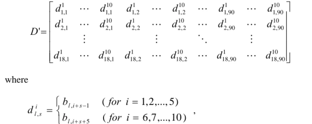
Recall the example discussed in previous section, the common site we want to find has 16 positions (ten ’s and six ignored letters), a sequence has 90 corresponding sites, so an 18*900 data matrix D’ is generated from D.

i

L

⎥ ⎥ ⎥ ⎥ ⎥ ⎦ ⎤ ⎢ ⎢ ⎢ ⎢ ⎢ ⎣ ⎡ = 10 90 , 18 1 90 , 18 10 2 , 18 1 2 , 18 10 1 , 18 1 1 , 18 10 90 , 2 1 90 , 2 10 2 , 2 1 2 , 2 10 1 , 2 1 1 , 2 10 90 , 1 1 90 , 1 10 2 , 1 1 2 , 1 10 1 , 1 1 1 , 1 ' d d d d d d d d d d d d d d d d d d D " " " " # % # # " " " " " " " " (2) where

⎩

⎨

⎧

=

=

=

+ + − +

)

10

,...,

7

,

6

(

)

5

,...,

2

,

1

(

5 , 1 , ,

_b

_for

_i

i

for

b

d

s i l s i l i s l ,

and s = 1…90 is the starting position of each candidate site.

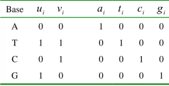
For {A, T, C, G}, two binary variables and can be used to express , an element of the consensus sequence, as shown in Tab. 1.

∈

i

L

u

_i

v

_i

L

_i

Tab. 1 indicates that if is A, T, C, or G respectively, then = 1, = 1, = 1 or = 1, which implies following conditions.

i

L

a

_i

t

_i

c

_i

g

_i (3)

)

1

(

)

1

(

)

1

)(

1

(

i i i i i i i i i i i i

v

u

g

v

u

c

v

u

t

v

u

a

−

=

−

=

=

−

−

=

Now let

Score

_l be the degree of fitting to the found common site, specified as

∑

= + + + = 90 1 10 , 2 , 1 , , ( ... ) s ls ls ls ls l z θ θ θ Score (4)

where is the element of candidate sites extracted from D’. The constraints associated with (4) are below:

i s l

(i)

∑

for all l and s. (5) = ∈ = 90 1 , , 1, {0,1} s s l s l z z (ii) (6) ⎪ ⎪ ⎩ ⎪ ⎪ ⎨ ⎧ = = = = = G C T A , , , , , i s l i i s l i i s l i i s l i i s l d if g d if c d if t d if a θ

Clearly,

0

≤

Score

_l

≤

10

. And the objective is to maximize the total sum of

Score

_l.

Consider the sample data in Fig. 1 for instance:

1

Score

= z1,1(a1+a2 +g3 +a4 +c5 +t6 +t7 +t8 +g9 +a10) (7) ) ( _{1 2 3 4 5 6 7 8 9 10} 2 , 1 a g a c t t t g a t z + + + + + + + + + + ) ( _{1 2 3 4 5 6 7 8 9 10} 3 , 1 g a c t g t g a t c z + + + + + + + + + +

Tab. 1. Base code in the determined common site

Base

u

_i

v

_i

a

_i

t

_i

c

_i

g

_i A 0 0 1 0 0 0 T 1 1 0 1 0 0 C 0 1 0 0 1 0 G 1 0 0 0 0 1

(a)

AAGACTGTTTTTTTGATC

GATTATTTGCACGGCGTC

(b)

l = 1, s = 1

AAGACTGTTTTTTTGATC

l = 1, s = 2

AAGACTGTTTTTTTGATC

l = 1, s = 3

AAGACTGTTTTTTTGATC

l = 2, s = 1

GATTATTTGCACGGCGTC

l = 2, s = 2

GATTATTTGCACGGCGTC

l = 2, s = 3

GATTATTTGCACGGCGTC

(c)

⎥

⎦

⎤

⎢

⎣

⎡

TTATTGCGTC

ATTATGGCGT

GATTACGGCG

GACTGTGATC

AGACTTTGAT

AAGACTTTGA

Fig. 1. A small example of finding consensus sequence: (a) two sequences to be compared;

(b) Schematic representation of the candidate sites; (c) The associated D’ matrix

2

Score

= z2,1(g1 +a2 +t3 +t4 +a5 +c6 +g7 +g8 +c9 +g10) (8) ) ( 1 2 3 4 5 6 7 8 9 10 2 , 2 a t t a t g g c g t z + + + + + + + + + + ) (1 2 3 4 5 6 7 8 9 10 3 , 2 t t a t t g c g t c z + + + + + + + + + +

All in (4) are binary variables. Equation (5) implies that for a sequence l, only one site is

chosen and no other sites contribute to . Suppose the k’th site is selected, then and

for all {1, 2, ..., 90}, . Since a huge amount of (i.e, s l z, l

Score

zl,k =1 0 ,s = l z

s

∈

s

≠

k

z_l,_s

l *

s

) are involved,

to treat as binary variables would cause a heavy computational burden. Therefore should be resolved as continuous variables rather than binary variables. An important proposition is introduced below:

s l

z, zl,s

Proposition 1 (All or nothing assignment) Let be continuous variables instead of binary variables. If there is a k, 0 ,s ≥ l z } 90 ..., , 2 , 1 { ∈ k , such that

, then assigning and

}

90

,...,

2

,

1

max{

10 1 , 10 1 ,

=

∑

=

∑

=

θ

i=

θ

for

s

i s l i i k l zl,k =1 zl,s =0

for all

s

≠

k

, s∈{1,2,...,90}, can maximize the value of

Score

_l.

Proof Since

∑

_, =1 and , it is true that

s

z

ls zl,s ≥0

∑

∑

∑

∑

≤ = = _i i k l i i s l s i i s l s l

θ

θ

s

θ

z

, , )} max{ , for 1,2,...,90} , ( { max

Remark 1 The objective function of a CSI problem f(x) can be rewritten as

∑

∑

∑

∑

∑

= ∈ ∈ ∈ ∈ + + + = 10 1 (, ) , ) , ( , ) , ( , ) , ( , } { ) ( i ls S s l i SC s l s l i ST s l s l i SA s l s l i i i i i

z

g

z

c

z

t

z

a

x

f

G (9) where , ,

, and for i=1,2,…10.

}

|

)

,

{(

l

s

d

_,

A

SA

i s l i

=

=

ST

{(

l

,

s

)

|

d

,

T

}

i s l i

=

=

}

|

)

,

{(

l

s

d

_,

C

SC

i s l i

=

=

SG

{(

l

,

s

)

|

d

,

G

}

i s l i

=

=

This result implies that (or , , ) is a set composed of (l, s) in which the product term (or , , respectively) appears on the right hand side of (4)

i

SA

ST

_i

SC

_i

SG

_i i s l a z, zl,sti zl,sci zl,sgi

because that

θ

_li_,s

=

a

_i.

For instance, the sum of

Score

₁ and

Score

₂ in (7) and (8) becomes

1

Score

+

Score

₂ = a1(z1,1+z1,2 +z2,2)+...+a10z1,1 1 , 2 10 1 , 2 3 , 1 1( ) ... ...+g z +z + +g z + (10)

Some logical constraints can be conveniently expressed by binary variables. For instance, the constraint that a CRP dimer binds a symmetrical site requires that

⎩

⎨

⎧

=

=

=

− −

G.

then

C

T,

then

A

if

11 11 i i i

L

L

L

Such a logical structure can be formulated conveniently as the following constraints.

}.

1

,

0

{

,

,

,

where

5

,

4

,

3

,

2

,

1

for

1

1

11 11 11 11

∈

=

⎭

⎬

⎫

=

+

=

+

− − − − i i i i i i i i

v

u

v

u

i

v

v

u

u

(11)

With reference to Tab. 1, clearly if

L

_i

=

A

(i.e,

u

_i

=

0

and

v

_i

=

0

) then (i.e, ) and vice versa; (ii) if

T

L

11_−i

=

1

and

1

11 11−i

=

v

−i

=

u

L

_i

=

C

(i.e,

u

_i

=

0

and

v

_i

=

1

) then (i.e,

) and vice versa. A CSI problem can then be formulated as a nonlinear mixed 0-1 program below based on these constraints:

G

L

11_−i

=

0

and

1

11 11−i

=

v

−i

=

u

Program 1 (Nonlinear 0-1 CSI program)

Maximize

∑

∑

∑

∑

∑

∑

= = ∈ ∈ ∈ ∈

+

+

+

=

18 1 10 1 (, ) , ) , ( , ) , ( , ) , ( ,

}

{

l i ls SG s l i SC s l s l i ST s l s l i SA s l s l i l i i i i

z

g

z

c

z

t

z

a

Score

(12) subject to 10 ..., , 2 , 1 for 1 , , , 0 10 ..., , 7 , 6 for 1 , 0 5 ..., , 2 , 1 for } 1 , 0 { , 5 ..., , 2 , 1 for s constraint Logical 1 1 10 ..., , 2 , 1 for s constraint ve Conservati ) 1 ( ) 1 ( ) 1 )( 1 ( all for 0 , 1 11 11 , 90 1 , = ≤ ≤ = ≤ ≤ = ∈ = ⎭ ⎬ ⎫ = + = + = ⎪ ⎪ ⎭ ⎪ ⎪ ⎬ ⎫ − = − = = − − = ≥ = − − =

∑

i g c t a i v u i v u i v v u u i v u g v u c v u t v u a s l, z z i i i i i i i i i i i i i i i i i i i i i i i i s l s s l

This program intends to solve { } for i =1,2, …10 thus to maximize the total degree of fitting to the common site for the given 18 sequences, subjected to a possible logical constraint. A

i i i i

t

c

g

very important feature of Program 1 is that we can treat as continuous variables rather than binary variables, which can improve the computational efficiency dramatically. We can ensure all found still have binary values as discussed in the next section.

s l z, s l z, Linearization of Program 1

Program 1 is a mixed nonlinear 0-1 program where

q

_i

∑

z

_l,s for and are product terms. These product terms can be linearized directly by the following propositions:

}

,

,

,

{

_{i i i i} i

a

t

g

c

q

∈

i i

v

u

Proposition 2 The product term

λ

_i

=

q

_i

∑

z

_l,s where

λ

_i is to be maximized and can be linearized as follows:

}

1

,

0

{

∈

i

q

(13) i i s l i i i s l i

q

M

z

q

M

z

≤

≤

≥

−

+

≥

∑

∑

λ

λ

λ

λ

, ,

0

)

1

(

where M is a big constant larger than or equal to the number of sequences. Proof If = 1 then

q

_i

λ

_i

=

∑

z

_l,s ; and otherwise

λ

_i= 0.

Proposition 3 The product term

w

_i

=

u

_i

v

_i where

u

_i

,

v

_i

∈

{

0

,

1

}

can be linearized as follows:

(14)

.

1

0

−

+

≥

≥

≤

≤

i i i i i i i i

v

u

w

w

v

w

u

w

Denote =

∑

_∈ , i SA s l ls i i a z a Z( ) _(,) , =

∑

_∈ i ST s l ls i i t z t Z( ) _(,) , , , and

. Program 1 is then linearized into Program 2 below based on Proposition 2 and Proposition 3.

∑

∈ = i SC s l ls i i c z c Z( ) _(,) ,

∑

∈ = i SG s l ls i i g z g Z( ) _{(, )} ,

Program 2 (Linear mixed 0-1 CSI program)

Maximize

∑

∑

= = + + + = 18 1 10 1 )) ( ) ( ) ( ) ( ( l i i i i i l Z a Z t Z c Z g Score (15)

subject to

10

...,

,

2

,

1

for

s

constraint

ve

Conservati

1

0

1

all

for

0

,

1

_, 90 1 ,

=

⎪

⎪

⎪

⎪

⎪

⎭

⎪

⎪

⎪

⎪

⎪

⎬

⎫

−

+

≥

≥

≤

≤

−

=

−

=

=

+

−

−

=

≥

=

∑

=

i

v

u

w

w

v

w

u

w

w

u

g

w

v

c

w

t

w

v

u

a

s

l,

z

z

i i i i i i i i i i i i i i i i i i i i s l s s l

5

...,

,

2

,

1

for

s

constraint

Logical

1

1

11 11

₌

⎭

⎬

⎫

=

+

=

+

− −

i

v

v

u

u

i i i i

rms

product te

g

linearizin

for

s

Constraint

)

(

0

)

(

)

1

(

)

(

0

)

(

)

1

(

)

(

0

)

(

)

1

(

)

(

0

)

(

)

1

(

) , ( , ) , ( , ) , ( , ) , ( , ) , ( , ) , ( , ) , ( , ) , ( ,

⎪

⎪

⎪

⎪

⎪

⎪

⎪

⎭

⎪

⎪

⎪

⎪

⎪

⎪

⎪

⎬

⎫

≤

≤

≤

≤

−

+

≤

≤

≤

≤

−

+

≤

≤

≤

≤

−

+

≤

≤

≤

≤

−

+

∑

∑

∑

∑

∑

∑

∑

∑

∈ ∈ ∈ ∈ ∈ ∈ ∈ ∈ i i SG s l ls i i SG s l ls i i SC s l ls i i SC s l ls i i ST s l ls i i ST s l ls i i SA s l ls i i SA s l ls

g

M

g

Z

z

g

Z

g

M

z

c

M

c

Z

z

c

Z

c

M

z

t

M

t

Z

z

t

Z

t

M

z

a

M

a

Z

z

a

Z

a

M

z

i i i i i i i i

10

...,

,

2

,

1

for

1

,

,

,

0

10

...,

,

7

,

6

for

1

,

0

5

...,

,

2

,

1

for

}

1

,

0

{

,

=

≤

≤

=

≤

≤

=

∈

i

g

c

t

a

i

v

u

i

v

u

i i i i i i i i s l

z, ’s are treated as non-negative continuous variables for l =1,2, … ,18 and s

=1,2, … ,90 where M can be any value greater than or equal to 18.

In Program 2, since and are binary variables, , , , and should have binary values following (3). Although are treated as continuous variables, the values of should be 0 or 1. This is because the optimal solution of a linear program should be a vertex point satisfying for all l.

i

u

v

_i

a

_i

t

_i

c

_i

g

_i s l z, zl,s

1

,

=

∑

s

z

ls

Proposition 4 Let the optimal solution of Program 2 be and . Assume

that a sequence l contains sites such that for j=1, 2, … k, then,

)

,

,

(

*

₌

∗ ∗ ∗

v

u

Z

x

∑

_,

=

1

s

z

ls k

s

s

s

₁

,

₂

,

...,

0

<

*_,

<

1

j s l

z

∑

∑

∑

∑

=

=

=

=

_i i s l i i s l i i s l i i s l,1

θ

,2

...

θ

,k

max{

θ

,

}

θ

,

(6)

in

specified

are

where

_li_,s j

θ

. Proof For

∑

_,

=

1

, if s

z

ls sp,sq∈{s1,s2,...sk} where

∑

>

∑

_i i s l i i s l, p

θ

, q

θ

, then to

maximize Scorel =

∑

_l,_jzl,sj

∑

_iθli,sj requires

z

l,sq

=

0

. This conflicts with the

observation that

0

<

_,

<

1

q

s l

z

, therefore

∑

_i

θ

_li,_s1

=

∑

_i

θ

_li,_s2

=

...

=

∑

_i

θ

_li,_sk .

After solving Program 2 we can obtain the globally optimum solution

“TGTGA□□□□□□TCACA” with objective value 147. The related nonzero values indicate the starting positions of the binding sites in the 18 sequences, as listed below:

s l z,

1

81 , 18 87 , 17 56 , 16 20 , 15 74 , 14 51 , 13 44 , 12 64 , 11 17 , 10 12 , 9 42 , 8 27 , 7 63 , 6 53 , 5 66 , 4 79 , 3 58 , 2 64 , 1

=

=

=

=

=

=

=

=

=

=

=

=

=

=

=

=

=

=

z

z

z

z

z

z

z

z

z

z

z

z

z

z

z

z

z

z

All other _zl,s’s have value 0.

In Program 2 the total number of 0-1 variables is 2m and the total number of the continuous variables is 20m+

l *

s

. Since the number of 0-1 variables is independent of the lengths of l and s, a CSI problem with many long sequences can be solved effectively.

Suboptimal common sites

Program 2 can find the exact global optimum solution. Sometimes the second best and the third best solution may also be useful. It is very convenient for the proposed method to find a complete set of common sites by adding some extra constraints. For instance, the second best solution of Program 2 can be obtained conveniently by solving the following program:

Maximize

∑

= 18 1 l l Score (16)

subject to

(i) The same constraints in Model 1

(ii)

t

1

+

g

2

+

t

3

+

g

4

+

a

5

+

t

6

+

c

7

+

a

8

+

c

9

+

a

10

≤

9

(new constraint)

The new constraint is used to force the program to find a new solution different from the solution of Program 2. The found second best common site is “TTTGA□□□□□□TCAAA” with score 129. Similarly we can find another solution by adding following constraint into (16).

9

10 9 8 7 6 5 4 3 2 1

+

t

+

t

+

g

+

a

+

t

+

c

+

a

+

a

+

a

≤

t

The found third best common site is “AAATT□□□□□□AATTT” with score 129.

3. Implementation

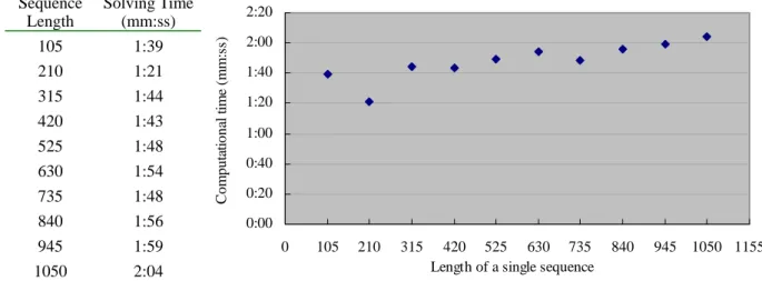
Several experiments are tested here, using the example in the Appendix, to analyze the effect of sequence length and number of sequences on the computational time. All examples are solved by LINGO (Schrage, 1999), a widely used optimization software, on a personal computer with a Pentium 4 2.0G CPU. A software package named “Global Site Seer” is developed based on Program 2 for solving CSI problems. This software is available from http://www.iim.nctu.edu.tw/~cjfu/gss.htm.

Fig. 2 illustrates the experimental results for analyzing the time complexity. Fig. 2(a) is the computational time given various sequence lengths, where the number of sequences is fixed at 18. The results show that the computational time changes slightly even if the sequence length is increased from 105 to 1050. Fig. 2(b) is the computational time with various numbers of sequences. It shows that the solving time is roughly proportional to the number of sequences. The proposed model is quite promising for treating CSI problems with large sequence length and a large number of sequence number. Fig. 2(c) shows that the computational time rises exponentially as the number of independent positions increases.

(a)

Computational time versus sequence length

Sequence Length Solving Time (mm:ss) 105 1:39 210 1:21 315 1:44 420 1:43 525 1:48 630 1:54 735 1:48 840 1:56 945 1:59 1050 2:04 0:00 0:20 0:40 1:00 1:20 1:40 2:00 2:20 0 105 210 315 420 525 630 735 840 945 1050 1155 Length of a single sequence

Com put at iona l t im e (m m :s s)

(b)

Computational time versus number of sequences

Number of Sequences Solving Time (mm:ss) 9 0:30 18 1:39 27 3:21 36 4:32 45 6:15 54 6:01 63 8:16 72 10:29 81 10:01 90 9:37 00:00 02:00 04:00 06:00 08:00 10:00 12:00 0 9 18 27 36 45 54 63 72 81 90 99 |l | : Number of sequences C o mp u tatio n al time ( mm:s s)

(c)

Computational time versus number of independent positions

Number of Indep Pos Solving Time (h:mm:ss) 2 0:00:01 3 0:00:03 4 0:00:21 5 0:01:23 6 0:03:38 7 0:05:18 8 0:08:25 9 0:15:52 10 0:53:27 11 2:33:20 0.1 1.0 10.0 100.0 1000.0 10000.0 100000.0 1 2 3 4 5 6 7 8 9 10 11 12 13

m : Number of independent positions

C o mp u tati o n al tim e (s ec o n d s)

Fig. 2.

The relationship between computational time and various factors involved in a CSI

problem. This figure illustrates the computational time of solving Program 2 with (a) various

sequences sizes; (b) various number of sequences and (c) various independent positions.

Time complexity and distributed computing

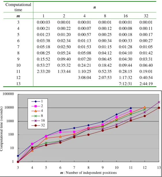
From the result of Fig. 2 we know that the time complexity is roughly proportional to the number of sequences and is influenced slightly by the length of sequences. However, the computational time rises exponentially as the number of independent positions increases. The worst case of time complexity of solving Program 2 on a single machine is estimated as O(

l

2

2m), where

l

is the number of sequences and m is the number of independent positions.

To treat CSI problems with more independent positions, a method of distributed computing is discussed in this section. Suppose there are n PCs available for solving Program 2, we can decompose Program 2 into n subprograms by specifying different values on some ’s and ’s. For instance, if

n = 32 then the first subprogram can be formulated as

i

u

v

_i Subprogram 1 Maximize

=

∑

l l

Score

x

f

(

)

(17) subject to

(i) The same constraint sets as in Program 2

(ii)

u

1

=

v

1

=

u

2

=

v

2

=

u

3

=

0

(new constraint)

The new constraint (ii) is used to reduce the number of 0-1 variables from 10 to 5. Similarly, constraint (ii) for the second subprogram can be set as

u

₁=1 and

v

₁

=

u

₂

=

v

₂

=

u

₃

=

0

. Constraint (ii) for the 32th subprogram could be

u

1

=

v

1

=

u

2

=

v

2

=

u

3

=

1

. All these 32 subprograms are solved simultaneously. Such a distributed computation algorithm can enhance the computational efficiency greatly. The computational time of Program 2 can be estimated as follows:

⎣log ⎦) 2 ( 2

2

)

,

,

(

l

m

n

l

m n

Time

=

_α

β − (18) where α and β are parameters, m is the number of independent positions, n is the number of

available PCs.

Fig. 3 is the results of some experiments for solving Problem 2 with various m and n while |l| = 18. For the example of finding CRP-binding sites, the estimated α and β values are α = 0.014 and β = 0.621.

Computational time n m 1 2 4 8 16 32 3 0:00:03 0:00:01 0:00:01 0:00:01 0:00:01 0:00:01 4 0:00:21 0:00:22 0:00:07 0:00:12 0:00:08 0:00:11 5 0:01:23 0:01:20 0:00:57 0:00:25 0:00:18 0:00:17 6 0:03:38 0:02:34 0:01:13 0:00:34 0:00:33 0:00:27 7 0:05:18 0:02:50 0:01:53 0:01:15 0:01:28 0:01:05 8 0:08:25 0:05:24 0:05:08 0:04:12 0:04:10 0:01:42 9 0:15:52 0:09:40 0:07:20 0:06:45 0:04:30 0:03:31 10 0:53:27 0:35:32 0:24:21 0:18:42 0:09:44 0:06:40 11 2:33:20 1:33:44 1:10:25 0:52:35 0:28:15 0:19:01 12 3:08:04 2:07:53 1:17:32 0:40:54 13 7:12:31 2:44:19 1 10 100 1000 10000 100000 3 4 5 6 7 8 9 10 11 12 13

m : Number of independent positions

Com put at io n al t im e (s ec onds ) 1 2 4 8 16 32

Fig. 3.

Computational time of distributed computing with various

m

(independent

positions) and

n

(number of available PCs)

A more complicated CSI problem is to search for the common site in an uncertain

pattern format where the number of ignored letters between the two half sites is unknown. An

example is to find a common site of length 2*5+k with the pattern

5 4 3 2 1

L

L

L

L

L

□

...

□

L

₆

L

₇

L

₈

L

₉

L

₁₀

where k, the number of

□

’s, is an unknown integer between 0 and 10.

Program 2 can be modified slightly to treat this type of extended CSI problems. Firstly

we expand D in (1) as D’ below:

D’ = [ D’(0) D’(1) D’(2) …… D’(10) ]

⎥ ⎥ ⎥ ⎥ ⎥ ⎦ ⎤ ⎢ ⎢ ⎢ ⎢ ⎢ ⎣ ⎡ = 10 , 90 , 18 1 , 90 , 18 10 , 2 , 18 1 , 2 , 18 10 , 1 , 18 1 , 1 , 18 10 , 90 , 2 1 , 90 , 2 10 , 2 , 2 1 , 2 , 2 10 , 1 , 2 1 , 1 , 2 10 , 90 , 1 1 , 90 , 1 10 , 2 , 1 1 , 2 , 1 10 , 1 , 1 1 , 1 , 1 ) ( ' k k k k k k k k k k k k k k k k k k d d d d d d d d d d d d d d d d d d k D " " " " # % # # " " " " " " " "

where

k∈{0,1,...,10}

.

⎩

⎨

⎧

=

=

=

− + + − +

)

10

,

9

,

8

,

7

,

6

for

(

)

5

,

4

,

3

,

2

,

1

for

(

1 , 1 , , ,

i

b

i

b

d

k s i l s i l i k s l i k s l .,

θ

=

a

_i

,

t

_i

,

c

_i

, or

g

_i

when

d

_li_,s.k

= ‘A’, ‘T’, ‘C’, or ‘G’ respectively.

The cases with k larger than 10 are not considered since they are relatively rare. A linear

mixed 0-1 program for solving this example is formulated below:

Program 3

Maximize

∑

= + + + m i i i i i Z t Z c Z g a Z 2 1 )) ( ) ( ) ( ) ( (

(15)

subject to

(i)

z z_lsk l,s k k k s k s l 1, , , 0 forall , 10 0 96 1 , , = ≥

∑ ∑

= − =

(ii)

∑

=

∑

=

=

∑

s k s s k s s k s

z

z

z

_{1, , 2,,}

...

_18,,

for

k∈{0,1,...,10}

(iii) the same conservative and logical constraints in Program 2

(iv) the same constraints for linearizing product terms in Program 2 but

replace

z_l,s

by

z_l,s.k

.

Constraints (i) and (ii) are used to ensure that when a specific k is chosen then

and

.

1

, ,

=

∑

s

z

lsk

∑

s

z

l,s,k'

=

0

for

k'

≠

k

Using Program 3 to search CRP binding sites we obtain the globally optimal solution as

“TGTGA□□□□□□TCACA” with score 147, which is exactly the solution found in

Program 2. And the second best solution is “GTGAA□□□□TTCAC” with score 134. The

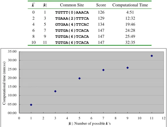
relationship between the computational time and the number of possible k’s (i.e. |k|) is linear,

as shown in the experiment result listed in Fig. 4. The number of ignored letter k is between 0

and

k ,

the upper bound of k, and thus we have |k| =

k

+ 1 in this experiment.

k |k| Common Site Score Computational Time 0 1 TGTTT(0)AAACA 126 4:51 2 3 TGAAA(2)TTTCA 129 12:32 4 5 GTGAA(4)TTCAC 134 19:46 6 7 TGTGA(6)TCACA 147 24:28 8 9 TGTGA(6)TCACA 147 25:49 10 11 TGTGA(6)TCACA 147 32:35 00:00 05:00 10:00 15:00 20:00 25:00 30:00 35:00 0 1 2 3 4 5 6 7 8 9 10 11 12 |k |: Number of possible k 's C o mp u tatio n al time ( mm:s s)

Fig. 4.

Computational time of Program 3 with various numbers of possible k’s. The

number enclosed in the common site is the solution of k.

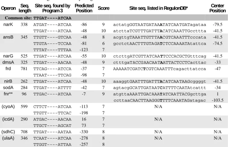
Finding FNR-binding sites

Program 3 is also applied to solve an example of searching for binding sites of fumarate

and nitrate reduction regulatory protein (FNR) in E. coli. Both CRP and FNR belong to the

CRP/FNR helix-turn-helix transcription factor superfamily (Tan et al., 2001). The sequence

data, which is taken from GenBank, contains 12 DNA sequences with lengths varied from 96

to 781. Owing to the dimer structure of the binding protein, the common site in this example

also has a constraint of inverse symmetry. The RegulonDB database (Huerta et al., 1998) lists

the found regulatory binding sites for eight of these twelve sequences while the exact

positions of other four sequences are not listed yet. Solving this example by Program 3 we

obtained the global optimal common site as “TTGAT

□□□□

ATCAA” with score 107,

which is the same common site as indicated by Tan et al. (2001). Tab.2 illustrates the result

including the common site and the predicted binding sites for all of the 12 sequences. Some

sites downstream of the transcription start (i.e. with positive indices) are also listed because

there are a few known cases in which regulatory sites appear within transcription units (Tan

et al., 2001). The proposed method has found some sites not listed in RegulonDB but having

scores higher than those listed in RegulonDB (e.g. the third solution in the Operon ansB row

of Tab.2). The best predicted sites in the four undetermined sequences are also listed in Tab.2.

5. Discussion

This study proposes a linear mixed 0-1 programming approach for solving CSI

problems. Comparing with the widely used maximum likelihood methods, the proposed

method can reach a global optimum rather than finding a local optimum or a feasible solution.

Additionally, by utilizing binary variables some logical constraints can be embedded into the

models. It is also convenient to find the complete set of the second, third, etc. best common

sites. Since the number of binary variables is fully independent of the number of sequences

and the length of a sequence, the proposed method can treat a large CSI problem with many

long sequences. For treating a CSI problem with many independent positions in an

acceptable time, this study also proposes a method for distributed computing.

The proposed method can also be conveniently extended to treat more complicated CSI

problems. In this study an extension of the linear program is designed to solve CSI problems

with an unknown number of ignored letters between the two half sites. The result of

searching for FNR-binding sites shows that the extended model can find not only the

locations of known binding sites listed in the RegulonDB database but also those not yet

Tab. 2.

FNR binding sites found by Program 3

Operon Seq. _length Site seq. found by _{Program 3} Predicted _{Position Score} Site seq. listed in RegulonDB* _Position Center

Common site: TTGAT----ATCAA

narK 338 ATGAT----ATCAA TTGAT----ATCAA -86 -48 9 10 actatgGGTAATGATAAATATCAATGATagataa atcttaTCGTTTGATTTACATCAAATTGccttta -79.5 -41.5 ansB 345 TTGTT----GTCAA TTGTA----TCCAA TTTAT----TTTAA -48 -81 -123 8 6 7 acgttgTAAATTGTTTAACGTCAAATTTcccata gcctctAACTTTGTAGATCTCCAAAATAtattca -41.5 -74.5

narG 525 TTGAT----ATCAA -55 10 ctcttgATCGTTATCAATTCCCACGCTGtttcag -41.5

dmsA 325 TTGAT----AACAA -48 9 ctttgaTACCGAACAATAATTACTCCTCacttac -33

frd 781 TTCAG----ATCCA TTAAT----TTCAG -37 -98 7 7 AAAAATCGATCTCGTCAAATTTcagacttatcca -47

nirB 262 TTGAT----ATCAA -48 10 aaaggtGAATTTGATTTACATCAATAAGcggggt -41.5

sodA 284 TTGAT----ATTTT -42 7 agtacgGCATTGATAATCATTTTCAATAtcattt -34

fnr** 96 TTGAC----ATCAA -7 9 atgttaAAATTGACAAATATCAATTACGgcttga ccttaaCAACTTAAGGGTTTTCAAATAGatagac 1 -103.5 (cyoA) 599 CTTCT----ATCAA TTGTT----TTCAC -113 -198 7 7 N/A N/A (icdA) 290 ATGAC----AACAA TTGCT----AGCAT 16 73 7 7 N/A N/A

(sdhC) 708 TTGAT----AATAA -330 8 N/A N/A

(ulaA) 346 TCAAT----ATCAA TTGGT----ATTAA -278 -257 8 8 N/A N/A

* For visualizing the comparison, the letters in uppercase represent the binding site listed in RegulonDB; the letter in bold face is the center of the site sequence; and the encompassed letters represent the exact binding site obtained by Program 3.

delimitated.

Two issues remaining for further study. The first is to extend this method to treat various

practical CSI problems. The second is to develop a more refined distributed algorithm to

solve some CSI problems by numerous computers via internet.

Appendix

The 18 unaligned DNA sequences containing CRP binding sites are used as the

example throughout this paper. It is taken from Stormo et al. (1989)

cole1 TAATGTTTGTGCTGGTTTTTGTGGCATCGGGCGAGAATAGCGCGTGGTGTGAAAGACTGTTTTTTTGATCGTTTTCACAAAAATGGAAGTCCACAGTCTTGACAG ecoarabop GACAAAAACGCGTAACAAAAGTGTCTATAATCACGGCAGAAAAGTCCACATTGATTATTTGCACGGCGTCACACTTTGCTATGCCATAGCATTTTTATCCATAAG ecobglr1 ACAAATCCCAATAACTTAATACTTGACATTTGTTATATATAACTTTATAAATTCCTAAAATTACACAAAGTTAATAACTGTGAGCATGGTCATATTTTTATCAAT ecocrp CACAAAGCGAAAGCTATGCTAAAACAGTCAGGATGCTACAGTAATACATTGATGTACTGCATGTATGCAAAGGACGTCACATTACCGTGCAGTACAGTTGATAGC ecocya ACGGTGCTACACTTGTATGTAGCGCATCTTTCTTTACGGTCAATCAGCAAGGTGTTAAATTGATCACGTTTTAGACCATTTTTTCGTCGTGAAACTAAAAAAACC ecodeop AGTGAATTATTTGAACCAGATCGCATTACAGTGATGCAAACTTGTAAGTAGATTTCCTTAATTGTGATGTGTATCGAAGTGTGTTGCGGAGTAGATGTTAGAATA ecogale GCGCATAAAAAACGGCTAAATTCTTGTGTAAACGATTCCACTAATTTATTCCATGGCACACTTTTCGCATCTTTGTTATGCTATGGTTATTTCATACCATAAGCC ecoilvbpr GCTCCGGCGGGGTTTTTTGTTATCTGCAATTCAGTACAAAACGTGATCAACCCCTCAATTTTCCCTTTGCTGAAAAATTTTCCATTGTCTCCCCTGTAAAGCTGT ecolac AACGCAATTAATGTGAGTTAGCTCACTCATTAGGCACCCCAGGCTTTACACTTTATGCTTCCGGATCGTATGTTGTGTGGAATTGTGAGCGGATAACAATTTCAC ecomale ACATTACCGCCAATTCTGTAACAGAGATCACACAAAGCGACGGTGGGGCGTAGGGGCAAGGAGGATGGAAAGAGGTTGCCGTATAAAGAAACTAGAGTCCGTTTA ecomalk GGAGGAGGCGGGAGGATGAGAACACGGCTTCTGTGAACTAAACCGAGGTCATGTAAGGAATTTCGTGATGTTGCTTGCAAAAATCGTGGCGATTTTATGTGCGCA ecomalt GATCAGCGTCGTTTTAGGTGAGTTGTTAATAAAGATTTGGAATTGTGACACAGTGCAAATTCAGACACATAAAAAAACGTCATCGCTTGCATTAGAAAGGTTTCT ecoompa GCTGACAAAAAAGATTAAACATACCTTATACAAGACTTTTTTTTCATATGCCTGACGGAGTTCACACTTGTAAGTTTTCAACTACGTTGTAGACTTTACATCGCC ecotnaa TTTTTTAAACATTAAAATTCTTACGTAATTTATAATCTTTAAAAAAAGCATTTAATATTGCTCCCCGAACGATTGTGATTCGATTCACATTTAAACAATTTCAGA ecouxul CCCATGAGAGTGAAATTGTTGTGATGTGGTTAACCCAATTAGAATTCGGGATTGACATGTCTTACCAAAAGGTAGAACTTATACGCCATCTCATCCGATGCAAGC pbr-p4 CTGGCTTAACTATGCGGCATCAGAGCAGATTGTACTGAGAGTGCACCATATGCGGTGTGAAATACCGCACAGATGCGTAAGGAGAAAATACCGCATCAGGCGCTC trn9cat CTGTGACGGAAGATCACTTCGCAGAATAAATAAATCCTGGTGTCCCTGTTGATACCGGGAAGCCCTGGGCCAACTTTTGGCGAAAATGAGACGTTGATCGGCACG (tdc) GATTTTTATACTTTAACTTGTTGATATTTAAAGGTATTTAATTGTAATAACGATACTCTGGAAAGTATTGAAAGTTAATTTGTGAGTGGTCGCACATATCCTGTT

References

Balas,E., Ceria,S. and Cornuéjols,G. (1996) Mixed 0-1 Programming by Lift-and-Project in a

Branch-and-Cut Framework. Management Science, 42, 1229-1246.

Brazma,A., Jonassen,I., Eidhammer,I. and Gilbert,D. (1998) Approaches to the automatic

discovery of patterns in biosequences. J. Comput. Biol., 5, 279-305.

Ecker,J.G., Kupferschmid,M., Lawrence,C.E., Reilly, A.A. and Scott, A.C.H. (2002) An

application of nonlinear optimization in molecular biology. European Journal of

unaligned DNA sequences known to be functionally related. Computa. Appl. Biosci., 6,

81-92.

Huerta,A.M., Salgado,H., Thieffry,D. and Collado-Vides,J. (1998) RegulonDB: a database on

transcriptional regulation in Escherichia coli. Nucl. Acids Res., 26, 55-59.

Lawrence,C.E. and Reilly,A.A. (1990) An expectation maximization (EM) algorithm for the

identification and characterization of common sites in unaligned biopolymer sequences.

PROTEINS: Structure, Function, and Genetics, 7, 41-51.

Schrage,L. (1999) Optimization Modeling With Lingo, LINDO Systems Inc., Chicago.

Stormo,G.D. and Hartzell,G.W. (1989) Identifying protein-binding sites from unaligned DNA

fragments. Proceedings of the National Academy of Sciences of the USA, 86, 1183-1187.

Stormo,G.D. (2000) DNA binding sites: representation and discovery. Bioinformatics, 16,

16-23.

Tan,K., Moreno-Hagelsieb,G., Collado-Vides,J. and Stormo,G.D. (2001) A comparative

genomics approach to prediction of new members of regulons. Genome Research, 11,

566-584.

八、計畫成果自評

1、 本研究已發展以全域最佳化方法求解 DNA 序列之共同區間定址問題，研究成果也已發表於 生物資訊之國際知名頂級期刊 Bioinformatics：

Han-Lin Li, and Chang-Jui Fu, “A Linear Programming Approach for Identifying a Consensus Sequence on DNA Sequences”, Bioinformatics, 21, 1838-1845, May 2005.

2、 本研究正陸續求解更深入的課題，並將於 INFORMS 2006 H.K. Conference 發表：

Han-Lin Li, and Chang-Jui Fu, “Identifying DNA Consensus Sequence Without Shared Patterns Using Linear Programs”, INFORMS International Conference, Hong Kong, June 25-28, 2006.