使用調適網格加密功能之有限元素平行化三維Poisson-Boltzmann Equation程式之發展與驗證

(1)

國

立

交

通

大

學

機

械

工

程

學

系

博士論文

使用調適網格加密功能之有限元素平行化三維

Poisson-Boltzmann Equation 程式之發展與驗證

Development and Verification of a 3-D Parallelized

Poisson-Boltzmann Equation Solver Using Finite

Element Method with Adaptive Mesh Refinement

研究生：邵雲龍

指導教授：吳宗信博士

(2)

使用調適網格加密功能之有限元素平行化三維

Poisson-Boltzmann Equation 程式之發展與驗證

Development and Verification of a 3-D Parallelized Poisson-Boltzmann Equation Solver Using Finite Element Method with Adaptive Mesh Refinement

研究生：邵雲龍 Student：Yun-Long Shao

指導教授：吳宗信博士 Advisor：Dr. Jong-Shinn Wu

國立交通大學

機械工程學系

博士論文

A Thesis

Submitted to Institute of Mechanical Engineering Collage of Engineering National Chiao Tung University

In Partial Fulfillment of the Requirements for the Degree of

Doctor of Philosophy in

Mechanical Engineering July 2006

Hsinchu, Taiwan, Republic of China

(3)

致謝

首先，感謝吳宗信教授這幾年的悉心教誨與熱心的指導，讓我在課業上或生活上均受益良多，在此表達由衷的感謝與敬意。且感謝各位口試委員：洪哲文教授、傅武雄教授、陳維新教授、江仲驊教授與黃楓南教授不吝指正，提出許多的寶貴意見，使得本論文的內容更加完備。同時要感謝MuST 所有的成員，包括國賢在理論與數值模擬上的大力協助、又永熱心協調平行計算設備資源的分配、允民在計算分析與欣芸在有限元素法技巧上的幫忙、捷粲在平行化程式上的協助、凱文在網格繪製上的幫助，以及坤樟、祐霖、哲維、富利熱情的鼓勵。此外，也要特別感謝已經畢業的碩士班學弟妹們的鼓勵與支持，讓我有源源不斷地動力繼續完成我的學業。最後，要感謝國家高速網路與計算中心提供叢集式電腦資源、國家奈米元件實驗室與交大奈米中心提供我學習相關設備的機會。邵雲龍謹誌 2006 年 07 月風城交大

(4)

Development and Verification of a 3-D Parallelized

Poisson-Boltzmann Equation Solver Using Finite

Element Method with Adaptive Mesh Refinement

Student：Yun-Long Shao Advisors：Dr. Jong-Shinn Wu

Department of Mechanical Engineering National Chiao Tung University

Abstract

Understanding of the interactive particle-particle and particle-wall forces in colloidal systems (electrolytes) plays a very important role in bio-chemistry related research. By assuming equilibrium in the electrolytes, the potential distribution with a very thin electrical double layer near the charged object can be well described by the well-known Poission-Boltzmann equation. Thus, a parallelized 3-D nonlinear Poisson-Boltzmann equation solver (PPBES) using finite element method (FEM) with parallel adaptive mesh refinement (PAMR) is proposed and verified. In this thesis, the research is divided into two phases, which are described as follows.

In the first phase, the nonlinear Poisson-Boltzmann equation is discretized using

Galerkin finite element method with unstructured tetrahedral mesh. Interpolation within a typical element includes the first-order and second-order shape functions. Inexact Newton iterative scheme is used to solve the nonlinear matrix equation resulting from the FE discretization. Jacobian matrix resulting from the Newton

(5)

easier parallel implementation. A parallel conjugate gradient (CG) method with a subdomain-by-subdomain (SBS) scheme is then used to solve the linear algebraic equation each iterative step. Completed code is verified using two typical examples. The first validated case is the potential distribution around a charged sphere. Excellent agreement of the simulation results with analytical (linearized case) and approximate (nonlinear case) solutions are obtained. The second validated case is the interaction between like-charged spheres within a cylindrical pore. Results show that the agreement between the present simulation and previous results are excellent. The above two typical simulations validate the present implementation of the PPBES. Further, the parallel performance is studied on a HP PC-cluster system at NCHC using a test case with a charged sphere confined in a cylindrical pore. Results show that 76.2% of parallel efficiency can be reached at processors of 32. Also FE discretization using the second-order shape function is demonstrated to be more accurate than using the first-order shape function at the end of this phase.

In the second phase, an h-refinement based PAMR scheme for an unstructured

tetrahedral mesh using dynamic domain decomposition on a memory-distributed machine is developed and tested in detail. A memory-saving cell-based data structure is designed such that the resulting mesh information can be readily utilized in both node- or cell-based numerical methods. The general procedures include isotropic refinement

(6)

from one parent cell into eight child cells and then followed by anisotropic refinement, which effectively removes the hanging nodes, with a simple mesh-quality control scheme. Parallel performance of this PAMR is studied on a PC-cluster system up to 64 processors. Results show that the parallel speedup scales approximately as N1.5_up

to 32 processors, where N is the number of processors. Then, procedure of coupling the PPBES with the PAMR using a posteriori error estimator is presented and verified using a test case with two like-charged spheres in a cylindrical pore. Results show that PAMR can systematically increase the solution accuracy of the PPBES. Finally, the coupled PPBES-PAMR code is used to simulate the interactive force between two like-charged spheres near a charged planar wall. Results are in excellent agreement with experimental data considering the experimental uncertainties, which is the first simulation in the literature to the best knowledge of the author.

Keywords: parallel Poisson-Boltzmann equation solver (PPBES), finite element method (FEM), parallel adaptive mesh refinement (PAMR), a posteriori error estimator.

(7)

使用調適網格加密功能之有限元素平行化三維

Poisson-Boltzmann Equation 程式之發展與驗證

學生：邵雲龍指導教授：吳宗信博士國立交通大學機械工程學系博士班

中文摘要

探討微粒-微粒與微粒-平板之間的相互作用力在生物化學的領域是相當重要的。在假設電解液為平衡的狀態下，可以經由著名的 Poisson-Boltzmann 方程式電雙層理論得到帶電物體的勢能分佈。因此，我們決定開發以有限元素法三維平行化非線性 Poisson-Boltzmann 方程式程式(PPBS)搭配平行化調適網格加加密功能程式(PAMR)，並且完成驗證的工作。本論文之研究分成兩大主軸，分別敘述如下：第一部分，以非線性 Poisson-Boltzmann 方程式採用非結構性四面體網格之葛勒金有限元素法來完成程式開發，包括了典型的一階與二階的形狀函數元素。

因為使用了nodal quadrature 的技巧，使得原先的牛頓法 Jacobian 矩陣僅剩下對

角線，以此擬牛頓疊代法來處理非線性項矩陣的部份，有助於平行化程式的完成。接下來，則使用SBS 的技巧搭配平行的共軛梯度法來處理線性矩陣方程組。完成的程式以兩個範例來驗證，第一個驗證的範例是帶電球體的勢能分佈，所得答案與解析解、近似解作一比較，結果相當正確。第二個驗證範例則是兩個帶電球體在圓柱孔內，結果顯示與先前所發表的論文結果相符。以上兩個驗證範例證明了平行化 Poisson-Boltzmann 方程式程式的開發完成。此外，平行化效能使用

(8)

國家高速網路與計算中心的HP 叢集式電腦系統來做驗證，測試一個帶電球體在圓柱孔內的範例，結果顯示使用了32 顆 CPU 時仍有 76.2%的平行效能。在第一部份的最後，我們使用了二階形狀函數元素，所得結果證明了比一階形狀函數元素要來的準確。 第二部份，主要是發展一個以非結構性四面體網格為主，採用 h-切割為基礎 之分散式記憶體動態領域分解的 PAMR 程式，而資料結構則使用了較節省記憶

體空間之cell-base 方式來記錄網格的資訊，可以同時運用在 node-base 與 cell-base

的數值方法上。一般的步驟包括了一個分為八個網格的等向性切割，然後以非等

向切割搭配網格品質控制將hanging node 有效率地移除。我們測試 PAMR 在叢

集式電腦上最多 64 顆 CPU 的平行化效能，結果呈現在 32 顆 CPU 時仍有 N1.5

的效能(N 為 CPU 個數)。接著我們將 PPBES 與 PAMR 做一個結合，並使用 a posteriori 的誤差評估方法，驗證兩個帶電球體在圓柱孔內，結果證明了使用

PAMR 可以增加 PPBES 解的準確度。最後，利用 PPBES-PAMR 的程式模擬兩個帶電球體靠近帶電平板的相互影響力之分析，與實驗結果相比較，若考慮實驗本身的不確定因素與誤差，模擬結果與實驗結果有相當程度的符合，這是目前已知與實驗結果相比較之最佳模擬結果。

關鍵字: 平行Poisson-Boltzmann方程式求解系統、有限元素法、平行搭配調適 網格功能、a posteriori誤差評估方法

(9)

List of Tables

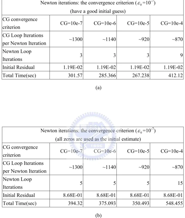
Table 3-1 The CG Solver and Newton Iteration for have a good initial guess and all

zeros are used as the initial estimate. (CPU=6; 81,354 nodes; 458,064 elements) ...84

Table 3-2 Analytical and approximate solutions for the simulation of the potential

distribution around a charged sphere. ...85

Table 3-3 The time breakdown (in seconds) for various components of the

parallelized Poisson-Boltzmann equations solver (electrostatic potential distribution around a charged sphere within a cylindrical pore; 106,390 nodes; 612,107 elements)...86

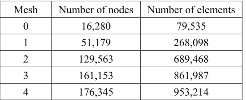
Table 3-4 The test mesh of number of nodes and elements for the second-order

element...87

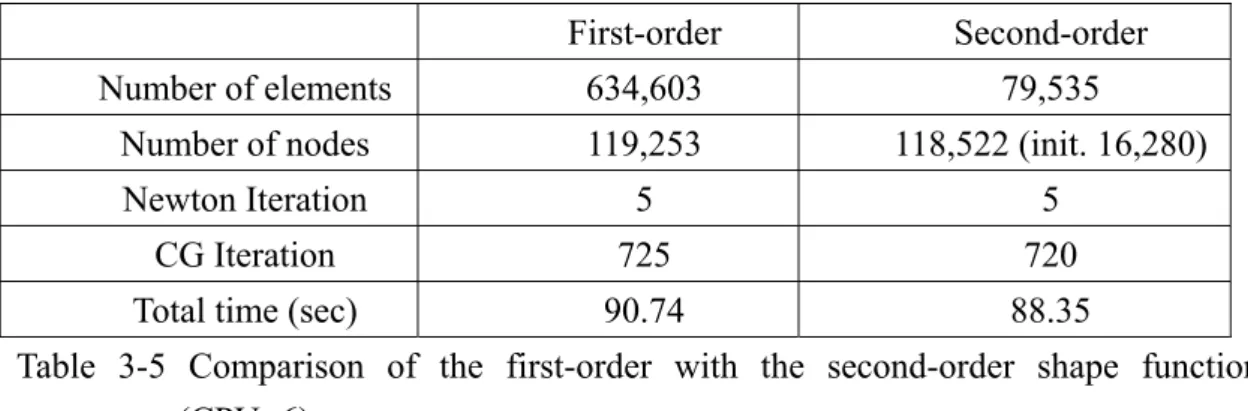
Table 3-5 Compare the first-order with the second-order element for level 0 (CPU=6)

...88

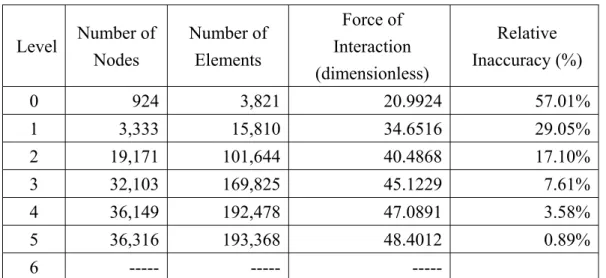
Table 4-1 Evolution of adaptive mesh refinement for computing force of interaction

between two charged spheres (radius=5) within a cylindrical pore (λ=0.416, 0003

. 0 =

pre

ε for a posteriori error estimator) use the first-order element. ...89

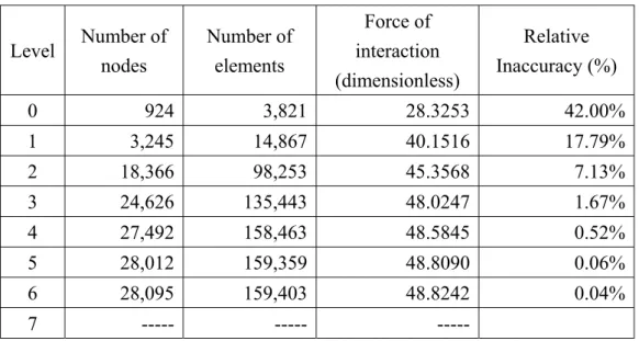
Table 4-2 Evolution of adaptive mesh refinement for computing force of interaction

between two charged spheres (radius=5) within a cylindrical pore (λ=0.416, 0003

. 0 =

pre

ε for a posteriori error estimator) use the second-order

element...90

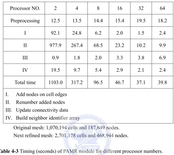
Table 4-3 Timing (seconds) of PAMR module for different processor numbers. ...91 Table 4-4 Evolution of force interaction between two identical charged spheres near a

like-charged flat plate (h=2.5μm, r=3μm, a=0.325μm and spheresΨ =3.0, ₀ flat plateΨ =5.0). ...92 ₀

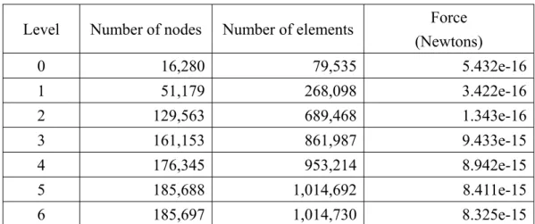
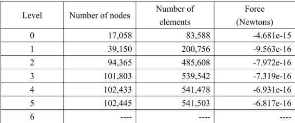
Table 4-5 Force of interaction with different refinement level mesh in the

simulation of two identical charged spheres near a charged flat plate

(h=2.5, r=4.5, a=0.325) for the first-order element...93

Table 4-6 Force of interaction with different refinement level mesh in the simulation

of two identical charged spheres near a charged flat plate (h=2.5, r=4.5, a=0.325) for the second-order element. ...94

(12)

List of Figures

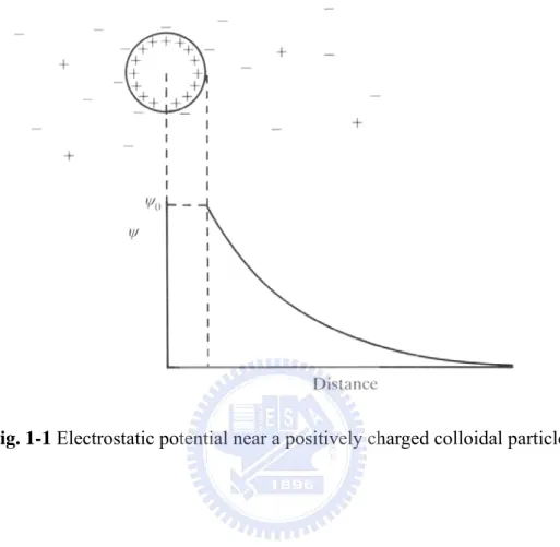
Fig. 1-1 Electrostatic potential near a positively charged colloidal particle...95

Fig. 1-2 The illustration of colloidal particle ...96

Fig. 1-3 The Electric Double Layer distribution...97

Fig. 1-4 p-refinement ...98

Fig. 1-5 r-refinement...99

Fig. 1-6 h-refinement ...100

Fig. 2-1 Three-dimensional tetrahedral element and face...101

Fig. 2-2 Interpolation functions of ten variable-number-nodes three-dimensional tetrahedral element...102

Fig. 2-3 Traditional shared memory multiprocessor model...103

Fig. 2-4 Distributed memory multiprocessor architecture...103

Fig. 2-5 PC cluster at MuST ...104

Fig. 2-6 The Poisson-Boltzmann equation solver by subdomains...105

Fig. 2-7 The flow chart of parallel Poisson-Boltzmann equation solver ...106

Fig. 3-1 The surface mesh distribution for the potential distribution of the a sphere (176309 elements; 36396 nodes) ...107

Fig. 3-2 Comparison of potential distributions around a charged sphere (a) surface potential Ψ =1.0 (b) surface potential ₀ Ψ =5.0 (18,253 nodes; 96,638 ₀ elements)...109

Fig. 3-3 The potential distribution for the sphere confined in a pore at separation distance r=6...110

Fig. 3-4 Potential along midplane between two spheres (r=6) ... 111

Fig. 3-5 The parallel speedup for the parallelized Poisson-Boltzmann equation solver for simulating the potential distribution around a charged sphere (radius=5) within a cylindrical pore (106,390 nodes; 612,107 elements)...112

Fig. 3-6 The distribution of potential around the charged spheres (radius a=0.325μm) near a like-charged plate (h = 2.5μm) at level-0 for solutions of (a) the first-order element (b) the second-order element...114

Fig. 3-7 The profiles of different mesh levels of the first-order element and the second-order element. the distribution of potential around the charged spheres (radius a=0.325μm) near a like-charged plate (distance h = 2.5μm) ...115 Fig. 3-8 The profiles of different mesh levels of the first-order element and the

second-order element (in local). the distribution of potential around the charged spheres (radius a=0.325μm) near a like-charged plate (distance h =

(13)

2.5μm)...116

Fig. 3-9 Potential along midplane between two spheres (r=6), compare the first-order element with the second-order element. (nodes 42,308 and elements 246,155) ...117

Fig. 4-1 Isotropic mesh refinement of tetrahedral mesh (T: Tetrahedron)...118

Fig. 4-2 Mesh refinement rules for two-dimensional triangular cell ...119

Fig. 4-3 Schematic diagram for mesh refinement rules of tetrahedron ...120

Fig. 4-4 Example of the common edge shared by the neighboring cells...121

Fig. 4-5 Schematic diagram of the proposed cell quality control ...122

Fig. 4-6 Schematic diagram of typical cell quality control...123

Fig. 4-7 A case that the proposed cell-quality-control would not affect to it...124

Fig. 4-8 Flow chart of parallel mesh refinement module...125

Fig. 4-9 Coupled PPBS-PAMR method...126

Fig. 4-10 The surface mesh distribution between two identical charged spheres (radius=5) in a cylindrical pore (λ=0.416) at (a) level-0 (initial; 924 nodes; 3,821 elements) (b) level-5 (final; 36,316 nodes; 193,368 elements) mesh refinement ...128

Fig. 4-11 Original (Level-3, 1,070,194 tetrahedral cells and 187,649 nodes) mesh distribution and next (Level-4, 2,701,178 cells and 468,944 nodes) refined mesh ...130

Fig. 4-12 Timing for different modules of PAMR at different processors...131

Fig. 4-13 Sketch of two identical charged spheres near a charged infinite flat plate 132 Fig. 4-14 The surface mesh distribution between two identical charged spheres (radius a=0.325μm) near a like-charged plate (h = 2.5μm) at the (a) level-0 (initial, 16,280 nodes; 79,535 elements) (b) level-5 (finial, 185,697 nodes; 1,014,730 elements) mesh refinement ...134

Fig. 4-15 The distribution of potential around the charged spheres (radius a=0.325μm) near a like-charged plate for (a) h = 2.5μm (b) h=9.5μm ...136

Fig. 4-16 Computed electrostatic force between charged spheres near a like-charged infinite flat plate as a function of the sphere center-to-center distance (h = 2.5μm for the second-order element. ...137

Fig. 5-1 Compare the code of tetrahedral mesh with the code of hybrid mesh of collapsed nodes ...138

(14)

Symbols

a The radius of the particle (m)

E The electric field vector

e The charge of a proton (C)

F The force acting on the spherical particle (Newton)

h The distance between plate and particle (m)

i

N FEM shape function

i

n Concentration of type i ion (m ) −3

0

i

n Bulk ionic concentration of type i ion (m ) −3

r The separation distance of particles (m)

T Absolute temperature ( K )

i

z Valence of type i ion

Greek symbols

ψ Electrical potential (V), and

T k ze b ψ ψ =

λ A cylindrical pore with the sphere radius to pore radius ratio

d

λ Debye length (m)

e

ρ The net charge density ( _{/ m}3

(15)

0 ε Permittivity of vacuum ( mV C ₎ κ Debye-Huckel parameter ( −1 m ) b κ Boltzmann constant (J /K)

δ The global absolute error

m

δ The current mean absolute error

pre

δ The prescribed global relative error ΔΠ The osmotic pressure

(16)

Chapter 1 Introduction

1-1 Motivation

Understanding of the electrostatic distribution in the electrical double layer (EDL) near charged particles or charged solid wall is crucial in understanding several important physical problems, including microscopic colloidal system [Okubo and Aotani,1998; Quddus and Moussa, 2004], electrokinetics in microfluidic system [Quddus and Moussa, 2004; Shao et. al., 2006; Collins and Lee, 2004], to name a few. Behavior of the EDL in a solution can be approximated by the nonlinear Poisson-Boltzmann equation (PBE). The Poisson-Boltzmann equation has been traditionally used to find the electrostatic potential around a macromolecule. Numerical investigation of models based on the PB equation can provide important information on effective particle interaction in colloidal systems.

The Poisson-Boltzmann equation is a second-order partial differential equation with a hyperbolic sine term that makes it exponentially nonlinear in the electrical double layer around the charged objects. Analytical solution is only possible for some problems with simple geometries and boundary conditions. However, most of the applications are three-dimensional with very complicated geometries, which necessitate the efficient and accurate numerical simulation of the Poisson-Boltzmann

(17)

three-dimensional Poisson-Boltzmann equation solver (PPBES) using the finite-element method (FEM), coupling with parallel adaptive mesh refinement (PAMR), which can be used efficiently and accurately for practical 3-D applications in the future.

1-2 Background

In this section, several important concepts about the microscopic colloidal behavior that is relevant to the Poisson-Boltzmann equation are described first. Then adaptive mesh refinement which is important to the accuracy and efficiency in solving the Poisson-Boltzmann equation is described in turn.

1-2-1 Poisson-Boltzmann Equation

1-2-1-1 Nature of Colloidal Solutions

Microscopic particles of one phase dispersed in another are generally called colloidal solution or dispersions. Three fundamental forces operate on fine particles in solution:

1. gravitational force, depending on particles density relative to the solvent; 2. viscous drag force, often described by Stoke’s Law, which depicts the force

(18)

velocity;

3. the ‘natural’ kinetic energy of particles and molecules.

The ‘natural’ kinetic energy including electrostatic force, which is an important factor of interaction for particles and molecules.

Fig. 1-1 shows the typical electrostatic potential distribution around a positively charged colloidal particle. Negative counter-ions are attracted towards the particle by the electric field generated by the positively charged surface, but they are also subject to thermal motion, which tends to spread then uniformly through the surrounding medium.

1-2-1-2 Zeta Potential

Almost all particulate or macroscopic materials in contact with a liquid acquire an electronic charge on their surfaces. Zeta potential is an important and useful indicator of this charge which can be used to predict and control the stability of colloidal suspensions or emulsions.

Colloidal particles dispersed in a solution are electrically charged due to their ionic characteristics and dipolar attributes. Each particle dispersed in a solution is surrounded by oppositely charged ions called the fixed layer shown as Fig. 1-2. Outside the fixed layer, there are varying compositions of ions of opposite polarities,

(19)

forming a cloud-like area. This area is called the diffuse double layer, and the whole area is electrically neutral in general.

When a voltage is applied to the solution in which particles are dispersed, particles are attracted to the electrode of the opposite polarity, accompanied by the fixed layer and part of the diffuse double layer, or internal side of the "sliding surface".

Zeta potential is considered to be the electric potential of this inner area including this conceptual "sliding surface". As this electric potential approaches zero, particles tend to aggregate.

1-2-1-3 Electric Double Layer

Electrokinetic phenomena are of considerable importance in many fields of science and engineering. In particular, they exert a strong influence on the flow behavior of a fluid, for example, in microchannels and capillaries.

The earliest studies of the electric double layer near a metal surface, by Helmholtz [Hunter, 1989] in the mid-nineteenth century, assumed that the electric charge on the metal surface was balanced by an equal charge which sat in the surrounding solutions a little way from the surface. Around 1910 a better model was proposed by a French scientist name Gouy and a similar treatment was developed

(20)

independently a few years later by the British scientist, Chapman. The result is known as the Gouy-Chapman model [Hunter, 1989] of the electric double layer, modified by Helmholtz model. It assumes that most solid surfaces bear electrostatic charges. When a charge surface is in contact with an electrolyte, the electrostatic charges on the solid surface will influence the distribution of nearby ions in the electrolyte solution. Ions of opposite of charges to that of the surface are attracted towards the surface, while ions of like charges are repelled from the surface; thus, an electric field is established. The charges on the solid surface and the balancing charge in the liquid are called the “electric double layer” (EDL). The EDL potential distribution is show in Fig 1-3. The sign and magnitude of the EDL field depend on the nature of the surface and the liquid.

Immediately next to the charged solid surface, there is a layer of ions that are strongly attracted to the solid surface and are immobile. This layer is called the compact or stern layer, normally about several Angstroms thick. The charge and potential distributions in this layer are mainly determined by the geometrical restriction of ion molecule size and the short-range interactions between ions, the wall and the adjoining dipoles.

From the compact layer to the electrically neutral bulk liquid, the net charge density gradually reduces to zero. Ions in this region are affected less strongly by the electrostatic interaction and are mobile. This region is called the diffuse layer of the

(21)

EDL. As will be discussed later, an equation called the Poisson-Boltzmann equation is used to describe approximately the ion and potential distributions in the diffuse layer.

The EDL width, called Debye length and afterward noted, determines the electric interaction range between macromolecules and therefore controls the static phase behavior of these systems.

1-2-1-4 Applications of Poisson-Boltzmann Equation

The Poisson-Boltzmann equation (PBE) provides a "fast" and approximate method for calculating the effects of solvent on electrostatic interactions in the modeled system. There are at least five major applications of the PBE:

1. Calculation of the electrostatic potential at the surface of a biomolecule, which is expected to give information about the concentration of small charged solutes in the neighborhood of the molecule and whose inspection may suggest docking sites for biomolecules [Bowen and Sharif, 1998]; 2. Calculation of the electrostatic potential outside the molecule, which is

expected to give information on the free energy of interaction of small molecules at different positions in the surrounding of the molecule. [Kozack and Subramaniam, 1993];

(22)

biomolecule which gives information on the stability of a biomolecule or of its different states [Sharp and Honig, 1990];

4. Calculation of the electrostatic field to derive mean forces to be added in standard molecular dynamics calculations [Gilson et. al., 1993].

5. Calculation of the electrostatic force among charged particles/walls, which is important in the study of colloidal system.

In the present thesis, we are mainly concerned about the last application of the Poisson-Boltzmann equation, to which it is not limited. The related derivation of Poisson-Boltzmann Equation will be discussed in chapter 2.

1-2-2 Adaptive Mesh Refinement (AMR)

Adaptive mesh refinement (AMR) is a computational technique for improving the efficiency and accuracy of solution of numerical simulations. In the AMR technique we start with a base coarse grid. As the solution proceeds we identify the regions requiring more resolution by some parameter characterizing the solution. We superimpose finer subgrids only on these regions. Finer and finer subgrids are added recursively until either a given maximum level of refinement is reached or the local truncation error has dropped below the desired level.

(23)

polynomial-degree-variation (p-refinement); (2) mesh movement (r-refinement); and (3) mesh enrichment (h-refinement), which will be briefly described respectively in the following.

1-2-2-1 Local Polynomial-Degree-Variation (p-refinement)

As shown in Fig. 1-4, local p-refinement scheme increases resolution of the solution by increasing the order of polynomial of the shape function in the element, which originated from finite element modeling. However, its implementation in three-dimensional finite-element modeling is rather complicated and not as popular as the mesh refinement (h-refinement) which will be introduced later.

1-2-2-2 Mesh Movement (r-refinement)

As shown in Fig. 1-5, the total mesh points remain the same in the computational domain after refinement. It is common to use a spring analogy, in which the nodes of the mesh are connected by springs whose stiffness is proportional to certain measure of solution activity over the spring. The mesh points are moved closer into the region where solution gradients are relatively large. This is often applied to the spatial adaptation of a structured mesh.

(24)

1-2-2-3 Mesh Enrichment (h-refinement)

As shown in Fig 1-6, with mesh enrichment, mesh points are added or embedded into the regions where relatively large solution gradients are detected, while the global mesh topology remains intact. It is generally regarded that mesh enrichment method has certain advantages over the first two methods. For example, the use of the h-refinement scheme generally does not impact the coding structure of the original

numerical scheme if hanging nodes are properly treated, while the use of p-refinement does, thus complicating the practical implementation. One of the most important advantages is that the mesh enrichment technique is in general many times faster and robust than the remeshing technique.

1-3 Literature Surveys

1-3-1 Numerical Simulation of Poisson-Boltzmann Equation

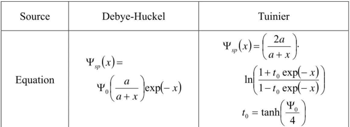
The Poisson-Boltzmann equation plays an important role in describing many physical phenomena, including like-charge particle interaction [Dyshlovenko, 2001; Squires and Brenner, 2000; Tuinier, 2003], particle-membrane interaction [Bowen, 1998; Tuinier, 2003], and electrokinetic flow [Yang et. al., 2001], among others. For example, one of the applications, colloidal dispersion, requires the knowledge of electrostatic potential distribution, which can then be used to calculate other quantities,

(25)

such as particle-particle interaction force. Features of particle interaction are of great importance for the stability and properties of colloidal dispersions. Accurate numerical modeling based on the Poisson-Boltzmann equation can provide important information on effective particle interaction in colloidal systems.

Bowen and Sharif [1997] presented a two-dimensional (axisymmetric) finite-element solution combined with adaptive mesh refinement. They used the Galerkin finite-element method with nine-node quadrilateral elements to discretize the Poisson-Boltzmann equation. The Newton-Raphson iterative scheme was used to handle the nonlinear hyperbolic sine term, while the Debye-Huckel solution was used as the initial guess Later, Bowen and Sharif [1998] applied the axisymmetric Poisson-Boltzmann equation solver to simulate the interactive force between two like-charge particles within a cylindrical pore with the same sign of charge on the surface. The results showed that at some inter-particle distance the two particles exhibit attractive forces, which is similar to that observed experimentally in Larsen and Grier [1997], although the magnitude is about one order different. It was then argued that in Ref. [Bowen and Sharif, 1998] the difference might be due to the fact that the wall is planar in the experiments [Larsen and Grier, 1997], whereas in the simulation it is cylindrical. For realistic applications like this, a three-dimensional simulation is required for accurate results. However, not only are 3D simulations extremely

(26)

time-consuming in practice, but developing efficient tools for them is also quite difficult.

Dyshlovenko [2001] also presented an axisymmetric Poisson-Boltzmann equation solver using finite-element method combined with adaptive mesh refinement. Instead of using nine-node quadrilateral elements, he used six-node triangular elements with a second-order shape function. Later, Dyshlovenko [2002] simulated the same problem as Bowen and Sharif [1998], but found no like-charge attractive force at any inter-particle distance in his simulation. In addition, Das and Bhattacharjee [2005] examined the effects of the roughness of the wall on the distribution of the electrostatic force using the two-dimensional finite-element method.

As shown in the above reviews, most existing studies use finite-element method with adaptive mesh refinement to solve the two-dimensional Poisson-Boltzmann equation. Very few studies have focused on developing a parallelized three-dimensional Poisson-Boltzmann equation solver even though the development of one would be valuable in understanding real physical phenomena. Two possible obstacles that have hindered the development of three-dimensional simulation are the time-demanding computation of a meaningful 3D simulation and the very complicated implementation of a parallel adaptive mesh refinement for a 3D unstructured mesh. Thus, it is important that to develop a parallelized three-dimensional

(27)

Poisson-Boltzmann equation solver using the Galerkin finite-element method using the first- and the second-order shape function combined with a parallel adaptive mesh refinement (PAMR) module.

1-3-2 Mesh Refinement

1-3-2-1 Adaptive Mesh Refinement

In previous section, we have briefly described three kinds of mesh refinement scheme: local polynomial-degree-variation (p-refinement), mesh movement (r-refinement) and mesh enrichment (h-refinement). As described earlier in previous section, the first [Zienkiewicz et. al., 1983; Peano, 1976] and second [Brackbill, 1993; Mackenzie and Robertson, 2002] methods have some disadvantages. Thus, comparatively few studies were conducted along these directions. It is generally regarded that mesh enrichment method (h-refinement) outperforms the first two methods [Rausch et. al., 1991]. One of the most important advantages is that the mesh enrichment technique is in general many times faster and robust than the re-meshing technique [Connell and Holms, 1994]. However, some disadvantages were mentioned in Ref.[Rausch et. al., 1991]. For example, appearance of the hanging nodes induces significant modification to the numerical method which couples the mesh refinement scheme. Fortunately, this can be overcome by some simple methods through the

(28)

elimination of hanging nodes, such as that proposed by Kallinderis and Vijayan [1993]. In the current study, we intend to employ similar technique to improve the accuracy of the Poisson-Boltzmann equation solver.

1-3-2-2 Parallel Adaptive Mesh Refinement (PAMR)

For treating large-scale simulation problems, not only we have to parallelize the numerical solver, but also we have to parallelize the mesh refinement scheme. There are several ways to classify PAMR algorithm, and some of them are reviewed in the following.

First, from the viewpoint of practical implementation on computers, PAMR can be generally categorized into two types: vectorized shared memory and distributed memory. In the shared memory type [Waltz, 2004], the hardware for parallel implementation is generally very expensive, and the coding is comparably easy, like using OpenMP [Chandra et. al., 2001], for instance. Memory access is direct and fast, which makes communication cost among processors minimal. Moreover, load balancing among processors is expected to be good, while memory contention may occur which possibly slows down the speed. In contrast, the hardware is more affordable for the distributed memory type than the shared memory type, while the coding is rather involved using MPI [Karypis et. al., 2003], for instance. Global data access is gained through network communication, which often becomes the bottleneck for better parallel performance if a large number of processors is used. However, this becomes increasingly unimportant because of the rapid increase in the

(29)

speed of network communication, and the dramatic reduction of costs in the past decade. Deciding on what type of parallel machine to implement greatly impacts the fundamental algorithm design as well as the practical implementation of the PAMR.

Second, from the viewpoint of the adaptive mesh refinement (AMR) algorithm itself, there are generally two kinds of mesh refinement: h-refinement and mesh regeneration. Mesh regeneration AMR [Wang and Harver, 1994] regenerates mesh from a mesh generator based on the distribution of error estimator obtained from the previous coarse mesh. For a large-scale 3-D computation, there exist two problems. First, the process often takes too much time, and second, the interpolation of previous solutions onto the new mesh is rather inefficient, which may slow down the convergence for the simulation on the new mesh. However, the data structure is relatively simple as compared to the h-refinement AMR. The h-refinement AMR adds grid points onto cell edges based on the error estimator obtained from the previous coarse mesh. It is generally much faster than the mesh regeneration type, and the interpolation onto the new mesh from the previous solution is straightforward, which may speed up the convergence for the computation on the new mesh. Often, the resulting “edge-based” data structure is very complicated and memory demanding, especially for the 3-D PAMR on the memory-distributed type of machine. Nevertheless, this type of AMR also has another advantage in that its data structure may be readily modified for mesh de-refinement, which may become important for a time-dependent simulation. Additionally, the h-refinement AMR possesses high spatial locality, which makes possible the parallel implementation on a memory-distributed machine using domain decomposition.

(30)

mesh data are required: the finite element type of connectivity (or connectivity) and cell-based connectivity (or cell neighbor-identifying information). The equation solver often needs the former, while the latter is required by some particle method for particle tracking, such as DSMC and PIC for solving the Boltzmann equation with neutral and charged species, respectively. However, the past development of the AMR scheme only produced the finite element type of connectivity. Related cell neighbor-identifying information can of course be obtained by post-processing serially (not in parallel) the node-based connectivity, while it may become time-consuming if the resulting mesh size is large. Thus, an ideal PAMR scheme may be expected to directly generate both these two sets of data.

For adaptive mesh refinement of three-dimensional tetartohedral mesh for the Poisson-Boltzmann equation, Cortis and Friesner [1997a, 1997b] proposed an automatic Finite-Element mesh generation system. Authors presented the algorithms of the construction of a tetrahedral mesh using a predetermined spatial distribution of vertices adapted to the geometry of the dielectric continuum solvent model. Besides, Baker[2000, 2001b] and his co-worker [Holst, 2000] publish the adaptive multilevel finite element treatment of the nonlinear PB equation using highly scalable parallel adaptive meshing methods which all of the numerical procedures are implemented in MANIFOLD CODE (MC) [web site, http://www.scicomp.ucsd.edu/ ~mholst/ codes/

(31)

mc/], a small self-contained parallel adaptive multilevel finite element software package.

1-4 Objectives of the Thesis

Based on previous reviews, the specific objectives of the thesis are summarized as follows:

1. To develop a parallelized 3-D Poisson-Boltzmann equation solver (PPBES) using finite element method with first- and second-order shape function on an unstructured tetrahedral mesh;

2. To develop a parallel adaptive mesh refinement (PAMR) for unstructured tetrahedral mesh;

3. To couple the PPBES and PAMR and apply it to compute a realistic 3-D problem.

1-5 Organization of the Thesis

The organization of this thesis is described as follows. Chapter 2 describes the numerical method for the parallelized Poisson-Boltzmann equation solver. Chapter 3 describes the validation and parallel performance study of the PPBES. Chapter 4 describes the proposed parallel adaptive mesh refinement, coupling scheme with

(32)

PPBES and application to a realistic 3-D problem. Finally, Chapter 5 describes the concluding remarks and recommendation of the future work. In addition, Appendix A describes the derivation of the nodal quadrature used in the present finite element formulation. Appendix B describes finite element formulation for hybrid mesh, which includes hexahedral, pyramid and tetrahedral mesh. Appendix C describes the first-order shape function of tetrahedral mesh and Appendix D describes the second-order shape function of tetrahedral mesh.

(33)

Chapter 2 Parallelized Poisson-Boltzmann Equation

Solver (PPBES) Using Finite-Element Method

In this chapter, derivation of the Poisson-Boltzmann equation is first demonstrated, followed by the discretization of the Poisson-Boltzmann equation using Galerkin finite element method, introduction to general conjugate gradient method for solving linear algebraic equation, inexact Newton iterative scheme and the parallel implementation of the finite-element discretization is deliberated in turn. Finally, formula of calculating electrostatic force used in the present thesis is shown

2-1 Theoretical Model and Analysis EDL

Consider a liquid phase containing positive and negative ions in contact with a planar negatively charged surface. An EDL field near a charged surface is established. According to the theory of electrostatics, the relationship between the electrical potential ψ and the net charge density per unit volume ρ_e at any point in the solution is described by the three-dimensional Poisson’s equation as

0 2 2 2 2 2 2 2 εε ρ ψ ψ ψ ψ e z y x ∂ =− ∂ + ∂ ∂ + ∂ ∂ = ∇ (2-1)

where ε is dielectric constant of the solution and ε₀ is permittivity of vacuum.

Applying the Boltzmann relation, assuming equilibrium, to the ionic number concentration distribution near a charged surface in a symmetric electrolyte solution (1:1), we have

(34)

) exp( 0 T k e z n n b i ψ − = + _and _exp( ₎ 0 T k e z n n b i ψ = − _(2-2)

Assuming the equilibrium Boltzmann distribution is reasonable, the number concentration of the type-i ion in a symmetric electrolyte solution is of the form

₀exp( ) T k e z n n b i i i ψ − = (2-3)

where n and _i₀ z are bulk ionic concentration and the valence of type-i ions, _i respectively, e is the charge of a proton, k is the Boltzmann constant, _b T is the absolute temperature, and exp( )

T k

e z

b

i ψ _{is the Boltzmann factor. The Boltzmann}

distribution is applicable only when the system is in the thermodynamic equilibrium state. Then the net charge density in a unit volume of the fluid is given by:

) sinh( 2 ) ( ₀ T k ze zen n n ze b e ψ ρ = +− − =− _(2-4)

For a symmetric 1:1 electrolyte system, substituting Equation (2-4) in Equation (2-1), a nonlinear second-order three-dimensional Poisson-Boltzmann equation is obtained as ) sinh( 2 0 0 2 2 2 2 2 2 T k ze zen z y x _b ψ εε ψ ψ ψ ₌ ∂ ∂ + ∂ ∂ + ∂ ∂ (2-5) By defining the Debye-Huckel parameter

T k n e z b 0 0 2 2 2 2 εε

κ = and applying the

dimensionless groups as follows, x x =κ , y=κy, z =κz and T k ze b ψ ψ =

The Poisson-Boltzmann equation, equation (2-5), can be re-written as: ) sinh( 2 2 2 2 2 2 ψ ψ ψ ψ ₌ ∂ ∂ + ∂ ∂ + ∂ ∂ z y x (2-6)

(35)

where 1κ (Debye length λ_d) is the characteristic length of the EDL.

Generally, solving this equation with appropriate boundary conditions, the electrical potential distribution ψ of the EDL can be obtained, and the local charge density distribution ρ_e can then be determined from equation (2-4). It should be noted that the Debye-Huckel parameter _κ2_{is independent of the solid surface}

properties and is determined by the liquid properties only, such as the electrolyte’s valence and the bulk ionic concentration.

2-2 Discretization Using Finite Element Method with Tetrahedral

Mesh

The FEM is the computer-aid mathematical technique for obtaining approximate numerical solution to the abstract of calculus that predicts the response of physical system subjected to the external influences.

Such problems arise in many areas of engineering, science, and applied mathematics. Applications to date have occurred principally in the areas of solid mechanics, heat transfer, fluid mechanics, and electromagnetism.

There are many salient features in FEM:

1. The domain is divided into smaller regions called elements. Adjacent elements touch without overlapping, and there are no gaps between the

(36)

elements. The shapes of the elements are intentionally made as simple as possible.

2. In each element the governing equations, usually in differential or variation (integral) form, are transformed into algebraic equation. The element equations are algebraically identical for all elements of the same type, which usually need to be derived for only one or two typical elements. 3. The resulting numbers are assembled (combined) into a much larger set of

algebraic equations called the system equations. Such huge systems of equations can be solved economically because the matrix of coefficients is “spares”.

4. Solved the matrix problem.

FEM seeks an approximate solution U~, an explicit expression for U, in terms of known functions, which approximately satisfies the governing equations and boundary conditions. It obtains an approximate solution by using the classical trial-solution procedure. Normally, it is not possible to obtain strong solutions for the problem at hand. Instead one usually decretive the otherwise continuous problem and obtain so-called weak solutions; weak in the sense of approximation.

(37)

the following six steps [Thompson, 2003; Zienkiweicz, 2000]: 1. Development of element equation.

2. Discretization of solution domain into a finite element mesh. 3. Assembly of element equations.

4. Introduction of boundary conditions. 5. Solution for nodal unknowns.

6. Computation of solution and related quantities over each element.

2-2-1 Interpolation with First-order Shape Function

In this section, we will describe the FE discretization of the three-dimensional nonlinear Poisson-Boltzmann equation using first-order shape function in detail. In general, the procedure are divided into the following steps.

Step1:

We use ψ~ to approximate ψ , then we set the trial solution:

∑

= = + + + = 4 1 ) ( 4 ) ( 4 3 ) ( 3 2 ) ( 2 1 ) ( 1 ) ( ₍ _, _, ₎ ~ j j e j e e e e e a z y x N a N a N a N a N ψ (2-7)

where x, y, z are the independent variables in the problems. The functions )

, , (x y z

N_j are known functions called trial functions (basis).

The purpose is to determine specific numerical values for each of the parameters

j

(38)

require that a weighted average of R(x,y,z) over the entire domain to be zero. The

weighting functions are trial functions N(x,y,z) associated with each a . _j Step2:

Applying Galerkin residual method, from Equation (2-6):

∫

Ω ∂ Ω= Ω Ω ∂ + ∂ ∂ + ∂ ∂ d N d z y x N_ie ( ₂ ) _i(e)sinh( ) 2 2 2 2 2 ) ( ψ ψ ψ _ψ _(2-8)

the Galerkin residual method is a weighting residual method, which uses the trial function as the weighting function. Thus, (e)

i

N is not only a weighting function, but

also a shape function. Note the integral

∫

ΩdΩ means integrate over the volume of element. In the present study, we employ tetrahedral elements, which have four degree of freedom (DOF) in each element.

Within the tetrahedral element, as shown in Fig.2-1, the function e i

ψ~ , the

first-order shape function, can be approximated as, z d y c x b a z y x _i e _i e _i e _i e e i ) *( ) *( ) *( ) *( ) ( ₍ _, _, ₎ ~ ₌ ₊ ₊ ₊ ψ , i=1~4 (2-9)

The coefficients *(e)

i

a , b_i*(e), c_i*(e) and d_i*(e) can be determined by enforcing Equation (2-9) at the four nodes of the element a unit value at each of the vertex. From which we can obtain,

) ( 6 1 6 1 ) ( 4 ) ( * 4 ) ( 3 ) ( * 3 ) ( 2 ) ( * 2 ) ( 1 ) ( * 1 ) ( ) ( 4 ) ( 3 ) ( 2 ) ( 1 ) ( 4 ) ( 3 ) ( 2 ) ( 1 ) ( 4 ) ( 3 ) ( 2 ) ( 1 ) ( 4 ) ( 3 ) ( 2 ) ( 1 ) ( ) ( * e e e e e e e e e e e e e e e e e e e e e e e e e e e a a a a V z z z z y y y y x x x x V a φ φ φ φ φ φ φ φ + + + = = (2-10)

(39)

) ( 6 1 1 1 1 1 6 1 ) ( 4 ) ( * 4 ) ( 3 ) ( * 3 ) ( 2 ) ( * 2 ) ( 1 ) ( * 1 ) ( ) ( 4 ) ( 3 ) ( 2 ) ( 1 ) ( 4 ) ( 3 ) ( 2 ) ( 1 ) ( 4 ) ( 3 ) ( 2 ) ( 1 ) ( ) ( * e e e e e e e e e e e e e e e e e e e e e e e b b b b V z z z z y y y y V b φ φ φ φ φ φ φ φ + + + = = (2-11) ) ( 6 1 1 1 1 1 6 1 ) ( 4 ) ( * 4 ) ( 3 ) ( * 3 ) ( 2 ) ( * 2 ) ( 1 ) ( * 1 ) ( ) ( 4 ) ( 3 ) ( 2 ) ( 1 ) ( 4 ) ( 3 ) ( 2 ) ( 1 ) ( 4 ) ( 3 ) ( 2 ) ( 1 ) ( ) ( * e e e e e e e e e e e e e e e e e e e e e e e c c c c V z z z z x x x x V c φ φ φ φ φ φ φ φ + + + = = (2-12) ) ( 6 1 1 1 1 1 6 1 ) ( 4 ) ( * 4 ) ( 3 ) ( * 3 ) ( 2 ) ( * 2 ) ( 1 ) ( * 1 ) ( ) ( 4 ) ( 3 ) ( 2 ) ( 1 ) ( 4 ) ( 3 ) ( 2 ) ( 1 ) ( 4 ) ( 3 ) ( 2 ) ( 1 ) ( ) ( * e e e e e e e e e e e e e e e e e e e e e e e d d d d V y y y y x x x x V d φ φ φ φ φ φ φ φ + + + = = (2-13) where ) ( 4 ) ( 3 ) ( 2 ) ( 1 ) ( 4 ) ( 3 ) ( 2 ) ( 1 ) ( 4 ) ( 3 ) ( 2 ) ( 1 ) ( 1 1 1 1 6 1 e e e e e e e e e e e e e z z z z y y y y x x x x

V = = volume of the element (2-14)

Thus, the coefficients *(e)

i

a , b_i*(e), c_i*(e) and d_i*(e) can be easily determined from expansion of the determinants and are not listed here for brevity. They can be found in Appendix C.

Substituting the expression for *(e)

a , b*(e), c*(e) and d*(e) back into Equation

(2-9), we obtain the interpolation function as given by: ) ( 6 1 ) , , ( N *() *() *( ) *() ) ( (e) j a b x c y d z V z y x = _e _je + _je + _je + _je (2-15)

(40)

as it should be. ⎩ ⎨ ⎧ ≠ = = = j i j i z y x _ij e i 0 1 ) , , ( N() _δ _(2-16)

and furthermore that N( )( , , ) z y x

e

i vanishes when the observation point is on the

surface of the tetrahedron opposite the j -th node. As a result, inter-element continuity of the interpolated function is guaranteed.

Step3:

Integrating Equation (2-8) by part, we can obtain

∑∫∫∫

= ∂ ∂ ∂ ∂ + ∂ ∂ ∂ ∂ + ∂ ∂ ∂ ∂ − ∂ ∂ ∂ ∂ + ∂ ∂ ∂ ∂ + ∂ ∂ ∂ ∂ i e e i i e i e e i e e i e e i e i e i e e i e dxdydz N dxdydz z N z y N y x N x dxdydz N z z N y y N x x ) sinh( ] ) ( ) ( ) [( )] ( ) ( ) ( [ ) ( ) ( ) ( ) ( ) ( ) ( ) ( ) ( ) ( ) ( ) ( ) ( ) ( ) ( ψ ψ ψ ψ ψ ψ ψ (2-17) Step4:

Applying Gauss divergence theorem to Equation (2-17), we can obtain

∑∫∫∫

∑∫∫

= ∂ ∂ ∂ ∂ + ∂ ∂ ∂ ∂ + ∂ ∂ ∂ ∂ − ⋅ ∂ ∂ + ∂ ∂ + ∂ ∂ i e e i i e i e e i e e i e j e i dxdydz N dxdydz z N z y N y x N x dxdy n N k z j y i x ) sinh( ] ) ( ) ( ) [( ˆ ] ˆ ˆ ˆ [ ) ( ) ( ) ( ) ( ) ( ) ( ) ( ) ( ) ( ψ ψ ψ ψ ψ ψ ψ (2-18)

Then, by substituting trial function, Equation (2-7), into Equation (2-18), we can obtain

(41)

∑∫∫∫

∑∑∫∫∫

∑∑∫∫

= ∂ ∂ ∂ ∂ + ∂ ∂ ∂ ∂ + ∂ ∂ ∂ ∂ − ⋅ ∂ ∂ + ∂ ∂ + ∂ ∂ i e e i j i e i j e j e i j e j e i j e j j i e i j e j j e j j e j dxdydz N dxdydz z N z a N y N y a N x N x a N dxdy n N k z a N j y a N i x a N ) ~ sinh( ] ) ( ) ( ) [( ˆ ] ˆ ˆ ˆ [ ) ( ) ( ) ( ) ( ) ( ) ( ) ( ) ( ) ( ) ( ) ( ) ( ψ (2-19) Now define: ) ˆ ˆ ˆ ( ˆ ) ( ) ( ) ( k z a N j y a N i x a N_je _j _je _j _je _j ∂ ∂ + ∂ ∂ + ∂ ∂ − = τ (2-20)

Equation (2-19) can be rewritten as follows,

∫∫

∑∫∫∫

∑∑∫∫∫

− − = ∂ ∂ ∂ ∂ + ∂ ∂ ∂ ∂ + ∂ ∂ ∂ ∂ dxdy dxdydz N dxdydz a z N z N y N y N x N x N n i e e i j j i e i e j e i e j e i e j τ ψ~ ) sinh( ] ) ( ) ( ) [( ) ( ) ( ) ( ) ( ) ( ) ( ) ( ) ( (2-21) or,

∫∫

∑∫∫∫

∑∑∫∫∫

− − = + + = = = dxdy dxdydz N dxdydz a d d c c b b V n i e e i j e i e j e i e j e i e j j i e τ ψ 4 1 ) ( ) ( ) ( * ) ( * ) ( * ) ( * ) ( * ) ( * 4 1 4 1 ( ) ) ~ sinh( ) ( 36 1 2 (2-22) where

∫∫∫

=_V(e) dxdydz (2-23)

Next, by substituting Equation (2-23) into Equation (2-22), we can obtain

∫∫

∑∫∫∫

∑∑

− − = + + = = = dxdy dxdydz N a d d c c b b V n i e e i j i j e i e j e i e j e i e j e τ ψ 4 1 ) ( ) ( 4 1 4 1 ) ( * ) ( * ) ( * ) ( * ) ( * ) ( * ) ( ) ~ sinh( ) ( 36 1 (2-24) Define

∑∑

= = + + = 4 1 4 1 ) ( * ) ( * ) ( * ) ( * ) ( * ) ( * ) ( ) ( ₍ ₎ 36 1 j i e i e j e i e j e i e j e e ij b b c c d d V K (2-25)

∫∫

∑∫∫∫

− − = = dxdy dxdydz N F _n i e e i e i ψ τ 4 1 ) ( ) ( ) ( _sinh(~ ₎ _(2-26)

(42)

Finally, we can obtain the matrix equation of the FE-discretized Poisson-Boltzmann Equation as

{ } { }

() ( ) ) ( _] [ e i e j e ij a F K = (2-27)

2-2-2 Interpolation with Second-order Shape Function

For some physical problems, tetrahedral elements with first-order shaper function are good enough for maintaining high accuracy. However, it may not be so for some problems like the present Poisson-Boltzmann equation due to the exponentially varying source term. Elements with higher order shape function are often necessary to improve the accuracy of the numerical solution, while the complexity of implementation and required memory increases with increasing order of shape function. Considering the compromise between numerical accuray and complexity of implementation, elements with the second-order shape function represents an optimum choice. Although the 4-node tetrahedron is the simplest solid element, they are not the preferred elements in engineering analysis because of their low accuracy. In what follows, elements with the second-order shape function are presented in detail.

The natural or tetrahedral coordinates system L₁, L₂ , L and ₃ L₄ of a

(43)

there are 10 nodal unknowns, 1 at each of the nodes as indicated in Fig. 2-2. The nodes 1, 2, 3 and 4 correspond to the corners, whereas the nodes 5 to 10 are located at the midpoints of the edges of the tetrahedron element. The variation of the field variable is given by

[ ]

[

]

( ) 10 2 1 ) ( ... ) , , (x y z = N Φe = N N N Φe φ (2-28)

where N can be found as _i

⎪ ⎪ ⎪ ⎪ ⎩ ⎪ ⎪ ⎪ ⎪ ⎨ ⎧ = = = = = = = − = 4 1 10 4 3 9 4 2 8 3 1 7 3 2 6 2 1 5 4 4 4 4 4 4 4 , 3 , 2 , 1 ), 1 2 ( N L L N L L N L L N L L N L L N L L N i L L_i _i i (2-29) and ⎪ ⎪ ⎭ ⎪ ⎪ ⎬ ⎫ ⎪ ⎪ ⎩ ⎪ ⎪ ⎨ ⎧ = = = = = = = = = = = = = ⎪ ⎪ ⎭ ⎪ ⎪ ⎬ ⎫ ⎪ ⎪ ⎩ ⎪ ⎪ ⎨ ⎧ = ⎪ ⎪ ⎭ ⎪ ⎪ ⎬ ⎫ ⎪ ⎪ ⎩ ⎪ ⎪ ⎨ ⎧ Φ Φ Φ = Φ ) 0 , 2 1 ( ) 0 , 1 ( ) 0 , 1 ( ) , , ( ) , , ( ) , , ( 2 1 4 3 4 3 1 2 4 3 2 1 ) ( 10 10 10 2 2 2 1 1 1 ) ( 10 2 1 ) ( L L L L at L L L L at L L L L at z y x z y x z y x e e e φ φ φ φ φ φ M M M (2-30)

Note that L is defined the same as Equation (2-15), but j N are replaced with i L . j

(44)

⎪ ⎪ ⎪ ⎭ ⎪⎪ ⎪ ⎬ ⎫ ⎪ ⎪ ⎪ ⎩ ⎪⎪ ⎪ ⎨ ⎧ + − + + − + + − = ⎪ ⎭ ⎪ ⎬ ⎫ ⎪ ⎩ ⎪ ⎨ ⎧ + + + ⋅ − + + + + ⋅ − + + + + ⋅ − = ∇ k L d j L c i L b V k y d c y d b d a d V z d j z d c y c b c a c V y c i z d b y c b b a b V x b V ] 2 2 1 [ ] 2 2 1 [ ] 2 2 1 [ 3 1 ] 2 2 2 3 ) 2 [( ] 2 2 2 3 ) 2 [( ] 2 2 2 3 ) 2 [( 18 1 1 * 1 1 * 1 1 * 1 * 1 * 1 * 1 * 1 * 1 * 1 * 1 2 * * 1 * 1 * 1 * 1 * 1 * 1 * 1 2 * 1 * 1 * 1 * 1 * 1 * 1 * 1 * 1 2 * 1 2 1 1 φ (2-31) and ) 4 1 2 4 ( 9 ) ( 9 ) 2 2 1 )( ( 1 2 1 2 2 * 1 2 * 1 2 * 1 2 2 1 2 * 1 2 * 1 2 * 1 1 1 + − + + = + − + + = ∇ ⋅ ∇ L L v d c b v L d c b φ φ (2-32)

By employing area coordinates, the volume integrals can be easily evaluated from the relation V d c b a d c b a dv L L L L V d c b a ₆ )! 3 ( ! ! ! ! 4 3 2 1 = ₊ ₊ ₊ ₊

∫

(2-33) Then,

∫∫∫

∇ ⋅∇ = + + 20 3 9 ) ( *2 1 2 * 1 2 * 1 1 1 v d c b dxdydz φ φ (2-34)

Some discussion of the derivation are shown in Appendix D and are not described here for brevity.

2-3 Conjugate Gradient Method for Linear Algebra Equation

The conjugate gradient method was developed in 1952 by Hestenes and Stiefel [1952] as an improvement to the steepest descent method. Whereas steepest descent

(45)

approaches the solution asymptotically, the conjugate gradient method will find the solution in n iterations (assuming no round-off error). There are many solvers including this method or subroutine presently [Holst et. al., 2000]. In our laboratory, the subroutine of conjugate gradient method of parallel version has developed by Hsu, K.-H [2006].

Generally, in the linear system Ax=b suppose the coefficient matrix A is

symmetric and positive definite. Solving Ax=b is equivalent to minimizing the

quadratic function Q x = xTAx−xTb 2

1 )

( . The conjugate gradient method is based on the idea that the convergence to the solution could be accelerates if we minimize Q over just the line that points down gradient. To determine i+1

x we minimize Q over ) , , , , ( 0 1 2 0 i p p p p span

x + _L , where the p represent previous search directions. An k added advantage to this approach is that, if we can select the k

p to be linearly

independent, then the dimension of the hyperplane will grow one dimension with each iteration of the conjugate gradient method. This would imply that (assuming infinite precision arithmetic) the solution of the linear system Ax=b would be obtained in

no more than N steps, where N is the number of unknowns in the system. Major algorithm in this method is summarized as:

For each process j;

(46)

step 2. 0 ₌0 j x , x_I0_j =0; r_j0 =b_j and r_I0_j =b_I_j step 3. Solve ( 0, 0 ) ( 0, 0 ) j I j j I j z r r z M = ; p0_j =z0_j, p_I0_j =z0_I_j step 4. 0 Pr ( 0, 0 ; 0, 0 ) j I j j I j z r r z oduct Inner r = Do k = 0, 1, 2…., Maximum Iterations step 5. ( , ) ( ,( , k )) j I k j k j I k j q MatrixMultiply A p p q = step 6. Pr ( 0, 0 ; 0, 0 ) j I j j I j k q q p p oduct Inner = τ step 7. k k k _r τ α = step 8. k j k k j k j r p x +1= +α ; x_Ik+1_j =r_Ik_j +αkp_Ik_j step 9. k j k k j k j r q r +1= −α ; r_Ik_j+1=r_Ik_j−αkq_Ik_j step 10. Solve ( +1, +1)₌( +1, k+1) j I k j k j I k j z r r z M step 11. +1 ₌ Pr ( +1, +1; +1, k+!) j I k j k j I k j k r r z z oduct Inner r

step 12. If ( rk+1 ≤Tolerance) END

step 13. k k k r r +1 = β ; k j k k j k j z p p +1 = +1+β , p_Ik+_j1 =z_Ik+_j1+βkp_Ik_j END DO

For parallel conjugate gradient method, in step 1 and step 5, the node-node of interface of subdomain need to do a communication. Besides, in step 6, all node of subdomain need to do one collective communication.

使用調適網格加密功能之有限元素平行化三維Poisson-Boltzmann Equation程式之發展與驗證

國

立

交

通

大

學

機

械

工

程

學

系

博士論文

使用調適網格加密功能之有限元素平行化三維

Poisson-Boltzmann Equation 程式之發展與驗證

Development and Verification of a 3-D Parallelized

Poisson-Boltzmann Equation Solver Using Finite

Element Method with Adaptive Mesh Refinement

研 究 生：邵雲龍

指導教授：吳宗信 博士

使用調適網格加密功能之有限元素平行化三維

Poisson-Boltzmann Equation 程式之發展與驗證

研 究 生：邵雲龍 Student：Yun-Long Shao

指導教授：吳宗信 博士 Advisor：Dr. Jong-Shinn Wu

國 立 交 通 大 學

機 械 工 程 學 系

博 士 論 文

致謝

Development and Verification of a 3-D Parallelized

Poisson-Boltzmann Equation Solver Using Finite

Element Method with Adaptive Mesh Refinement

Abstract

使用調適網格加密功能之有限元素平行化三維

Poisson-Boltzmann Equation 程式之發展與驗證

中文摘要

Table of Contents

List of Tables

List of Figures

Symbols

Chapter 1 Introduction

1-1 Motivation

1-2 Background

1-3 Literature Surveys

1-4 Objectives of the Thesis

1-5 Organization of the Thesis

Chapter 2 Parallelized Poisson-Boltzmann Equation

Solver (PPBES) Using Finite-Element Method

2-1 Theoretical Model and Analysis EDL

2-2 Discretization Using Finite Element Method with Tetrahedral

Mesh

∑

∫

∫

∫

∑∫∫∫

∑∫∫∫

∑∫∫∫

∑∫∫∫

∑∫∫∫

∑∫∫

∑∫∫∫

∑∑∫∫∫

∑∑∫∫

∫∫

∑∫∫∫

∑∑∫∫∫

∫∫

∑∫∫∫

∑∑∫∫∫

∫∫∫

∫∫

∑∫∫∫

∑∑

∑∑

∫∫

∑∫∫∫

{ } { }

[ ]

[

研究生：邵雲龍

指導教授：吳宗信博士

研究生：邵雲龍 Student：Yun-Long Shao

指導教授：吳宗信博士 Advisor：Dr. Jong-Shinn Wu

國立交通大學

機械工程學系

博士論文