Temperature Prediction Using Fuzzy Time Series
Shyi-Ming Chen, Senior Member, IEEE, and Jeng-Ren Hwang
Abstract—A drawback of traditional forecasting methods is that
they can not deal with forecasting problems in which the historical data are represented by linguistic values. Using fuzzy time series to deal with forecasting problems can overcome this drawback. In this paper, we propose a new fuzzy time series model called the two-factors time-variant fuzzy time series model to deal with fore-casting problems. Based on the proposed model, we develop two algorithms for temperature prediction. Both algorithms have the advantage of obtaining good forecasting results.
Index Terms—Main-factor fuzzy time series, second-factor fuzzy
time series, temperature prediction, time-invariant fuzzy time se-ries, time-variant fuzzy time series.
I. INTRODUCTION
I
T is obvious that forecasting activities play an important role in our daily life. Every day the weather forecast tells us what the weather will be like tomorrow. We can prevent huge damage by forecasting the coming of storms or typhoons. We usually forecast many things concerned with our daily life, such as economy, stock market, population growth, weather, etc. To make a forecast with 100% accuracy may be impossible, but we can do our best to reduce the forecasting errors or increase the speed of the forecasting process. To solve the forecasting prob-lems, many researchers have proposed many different methods or models. A drawback of traditional forecasting methods is that they can not deal with forecasting problems in which the historical data are linguistic values. In order to overcome the drawback of the traditional forecasting methods, in [17], Song and Chissom proposed the concepts of fuzzy time series to deal with the forecasting problem in which the historical data are lin-guistic values. In [18] and [19], they proposed two fuzzy time series models to deal with the forecasting problems for fore-casting enrollments of the University of Alabama.In [18], Song et al. use the following method to forecast en-rollments of the University of Alabama:
(1) where
fuzzified enrollment of year ;
forecasted enrollment of year represented by fuzzy sets;
Manuscript received May 13, 1998; revised January 5, 2000. This work was supported in part by the National Science Council, R.O.C., under Grant NSC 85-2213-E-009-123. This paper was recommended by Associate Editor A. Kandel.
S.-M. Chen is with the Department of Electronic Engineering, National Taiwan University of Science and Technology, Taipei, Taiwan, R.O.C.
J.-R. Hwang is with the Department of Computer and Information Science, National Chiao-Tung University, Hsinchu 300, Taiwan, R.O.C.
Publisher Item Identifier S 1083-4419(00)02965-4.
union of fuzzy relations; “ ” Max-Min composition operator.
It takes a lot of time to compute the union of fuzzy relations , but it is computed only once. In [19], Song et al.proposed the time-variant fuzzy time series model. The model also uses (1), but the calculation of the union of fuzzy relations is different from the method in [18]. The method presented in [19] takes less time to compute the union of fuzzy relations , but it must recalculate when we want to forecast the enrollments of dif-ferent years. The time complexities of the methods in [18] and [19] are all , where is the number of fuzzy logical re-lationships, and is the number of elements in the universe of discourse. Although some researchers have proposed new fuzzy time series models to improve Song's model, such as [4], [5], [7], and [21], all of these models can only deal with one-factor fore-casting problems. In [4], we presented a time-invariant fuzzy time series method to forecast university enrollments. In [5], Day proposed a time-variant fuzzy time series model which used expert opinions and genetic algorithms. In [7], we presented a one-factor time-variant fuzzy time series model and proposed an algorithm for handling forecasting problems. In [21], Sul-livan et al. proposed the Markov model which used linguistic labels with probability distributions.
In this paper, we propose a new fuzzy time series model which is called the “two-factors time-variant fuzzy time series model” to deal with forecasting problems. Based on the proposed model, we develop two algorithms for temperature prediction. The proposed algorithms have the advantage that they can obtain good forecasting results.
The rest of this paper is organized as follows. In Section II, we briefly review some basic concepts of fuzzy set theory [8]–[11], [28] and fuzzy time series [17]–[19]. In Section III, we propose the two-factors time-variant fuzzy time series model and pro-pose two efficient algorithms for temperature prediction. The conclusions are discussed in Section IV.
II. FUZZYSETTHEORY ANDFUZZYTIMESERIES
In the following, we briefly review some basic concepts of fuzzy set theory from [8]–[11], and [28]. A fuzzy set is a class with fuzzy boundaries. A fuzzy set can be characterized by a membership function defined as follows.
Definition 2.1: Let be the universe of discourse. A fuzzy subset on the universe of discourse can be defined as fol-lows:
(2)
where is the membership function of ,
and is the degree of membership of the element in the fuzzy set .
Definition 2.2: Let be the universe of discourse, , and be a finite set. A fuzzy set can be expressed as follows:
(3)
where the symbol “ ” means the operation of union instead of the operation of summation, and the symbol “ ” means the seperator rather than the commonly used algebraic symbol of division.
Definition 2.3: Let be the universe of discourse, where is an infinite set. A fuzzy set of can be expressed as follows:
(4)
Definition 2.4: Let be a fuzzy set of the universe of dis-course . The -significance level [27] of the fuzzy set is defined as follows:
if
otherwise (5)
where .
The concept of fuzzy time series was proposed by Song et
al. [17]. In a traditional time series, the values of observations
of a special dynamic process are represented by crisp numerical values. However, in a fuzzy time series, the values of observa-tions of a special dynamic process are represented by linguistic values. In [18] and [19], Song et al. used the fuzzy time series to forecast the enrollments of the University of Alabama, and they got good forecasting results. In the following, we briefly review the concept of fuzzy time series from [17].
Definition 2.5: Assume that is
a subset of real numbers and is the universe of discourse, and
assume that fuzzy sets are defined on .
Let be a collection of . Then, is
called a fuzzy time series of .
We can see that is a function of time , and
are linguistic values of , where are
represented by fuzzy sets. In [17], Song et al.divided the fuzzy time series into two categories which are the time-invariant fuzzy-time series and the time-variant fuzzy time series defined as follows.
Definition 2.6: If is caused by denoted by , then this relationship can be represented by
(6)
where is a fuzzy relationship between and and is called the first-order model of .
Definition 2.7: Assume that is a fuzzy time series, and is a first-order model of . If
for any time , then is called the time-invariant fuzzy time series. If is dependent on time , that is may be different from for any , then is called the time-variant fuzzy time series.
In [18], Song and Chissom proposed the time-invariant fuzzy time series model. In [19], Song et al. proposed the time-variant fuzzy time series model. Both of these two models only used one factor to forecast the enrollments of the University of Al-abama. In fact, an event may be influenced by many factors. In the following, we propose a new fuzzy time series called the two-factors fuzzy time series.
Definition 2.8: Assume that fuzzy time series and are the factors of the forecasting problems. If we only use to solve the forecasting problems, then it is called a one-factor fuzzy time series. If we use both and to solve the forecasting problems, then it is called a two-factors fuzzy time series.
III. A NEWFUZZY TIME SERIES MODEL FOR
TEMPERATUREPREDICTION
In [7], we have presented a one-factor time-variant fuzzy time series model and proposed an algorithm (called Algorithm-A) for handling the forecasting problems. However, in the real-world, an event can be affected by many factors. For example, the temperature can be affected by the wind, the sunshine dura-tion, the cloud density, the atmospheric pressure, , etc. If we only use one factor of them to forecast the temperature, the fore-casting results may lack accuracy. We can get better forefore-casting results if we consider more factors for temperature prediction. In [4], [18], [19], and [21], the researchers only use the one-factor fuzzy time series model to deal with the forecasting problems. In this section, we propose a new forecasting model which is a two-factors time-variant fuzzy time series model. Based on the proposed model, we develop two algorithms which use two factors (i.e., the daily average temperature and the daily cloud density) for temperature prediction.
Definition 3.1: Assume that
is a subset of and is the universe of discourse. Let
and be two fuzzy time series
on , where
is a fuzzy set on is a fuzzy set on , and . Assume that we want to forecast and use to aid the forecasting of , then and are called the main-factor fuzzy time series and the second-factor fuzzy time series of the two-factors time-variant fuzzy time series model, respectively.
For example, in the proposed two-factors time-variant fuzzy time series model for temperature prediction, “the daily average temperature” and “the daily cloud density” are called the main-factor and the second-factor of the two-factors time-variant fuzzy time series model, respectively.
The fuzzified variation of the main-factor fuzzy time series between time and time can be described as follows. Assume that the universe of discourse has been
divided into m intervals (i.e., and ). Furthermore, assume that there are linguistic terms (i.e., and
) described by fuzzy sets shown as follows:
.. .
(7) where the maximum membership value of occurs at and . If the difference of the historical data of the main-factor fuzzy time series between time and time is and , then the fuzzified variation of the historical data of the main-factor fuzzy time series between time and time is , where . That is,
The fuzzified data of the second-factor fuzzy times series at time can be described as follows. Assume that there are linguistic terms (i.e., and ) represented by fuzzy sets to describe the fuzzified historical data of the second-factor “the daily cloud density”, where the daily cloud density ranges from 0% to 100%
.. .
(8) If the data of the second-factor fuzzy time series , then the fuzzified data of is . If , then the fuzzified data of is . If , then the fuzzified data of is . If , then the fuzzified data of is . If , then the fuzzified data of is . If
, then the fuzzified data of is . If , then the fuzzified data of is .
To forecast the data of time , we must decide the window basis . Then, we can get the criterion vector and the op-eration matrix at time which are expressed as follows: (9)
.. .
..
. ... ... ... (10)
where is the fuzzified variation of the main-factor fuzzy time series between time and time is the
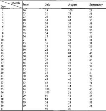
TABLE I
HISTORICAL DATA OF THE DAILY
AVERAGETEMPERATURE FROMJUNE1996TOSEPTEMBER1996
INTAIPEI(UNIT: C) [2]
number of elements in the universe of discourse, and
are crisp values, ,
and .
From (9) and (10), we can see that both the criterion vector and the operation vector are caused by the main-factor fuzzy time series . In the following, we define the second-factor vector which is composed by the second-factor fuzzy time series .
Definition 3.2: Let be a second-factor fuzzy time series in the universe of discourse. The second-factor vector is described by
(11) where is the second-factor vector at time is the fuzzified data of the second-factor fuzzy time series at time is the number of elements in the universe of discourse,
, and .
The fuzzy relationship of the one-factor time-variant fuzzy time series model is the relationship between the operation matrix and the criterion matrix. In the two-factors time-variant fuzzy time series model, we must decide the fuzzy relationship between the criterion vector, the operation matrix, and the second-factor vector. The new fuzzy relationship matrix is defined as follows.
Definition 3.3: Assume that is the main-factor fuzzy time series and is the second-factor fuzzy time series, is a criterion vector on is an operation matrix on
re-TABLE II
HISTORICALDATA OF THEDAILYCLOUDDENSITY FROMJUNE1996TO
SEPTEMBER1996INTAIPEI(UNIT: %) [2]
lationship matrix between , and is equal
to , where we have (12), shown
at the bottom of the page. is the number of elements in the universe of discourse,
, and “ ” is the multiplication operator.
From the fuzzy relationship matrix , we can get the fuzzi-fied forecasted variation between time and time de-scribed by
(13) where is the fuzzified variation of the fuzzy time series
between time and time .
TABLE III
FUZZIFIEDHISTORICALDATA OF THEMAIN-FACTOR(THEDAILYAVERAGE
TEMPERATURE)AND THESECOND-FACTOR(THEDAILYCLOUDDENSITY)
INJUNE1996INTAIPEI
In the following, we propose a new algorithm called Algo-rithm-B based on the proposed two-factors time-variant fuzzy time series model and we will use two factors (i.e., the daily average temperature and the daily cloud density) for tempera-ture prediction from June 1996 to September 1996 in Taipei, Taiwan, where “the daily average temperature” and “the daily cloud density” are called the main-factor and the second-factor of the two-factors time-variant fuzzy time series model, respec-tively. The algorithm is now presented as follows.
Algorithm-B:
Step 1) Partition the historical data into suitable groups and perform the following forecasting steps to each group, respectively. For example, we partition the historical data into four groups, i.e., June, July, August, and September, as shown in Table I.
..
. ... ... ...
..
Fig. 1. Curve of the actual temperature and forecasted temperature of Algorithm-A with the window basesw = 2 and w = 3.
Step 2) Compute the variations of the main-factor fuzzy time series between any two continuous data. Find the maximum decrease and the maximum increase between any two continuous data, and define the
universe of discourse ,
where and are suitable positive numbers. For example, assume that we want to forecast the tem-perature of June 1996 in Taipei. From Table I, we
can see that , and . We set
. Then, the universe of discourse
can be defined as .
Step 3) Partition the universe of discourse into
sev-eral even length intervals . For
example, in this case, we partition the universe of
discourse into seven intervals ,
where
, and .
Step 4) Define fuzzy sets on the universe of discourse for the fuzzified variation of the main-factor fuzzy time series . In this case, we consider seven fuzzy sets which are very big decrease big
decrease decrease no change
increase big increase very big
increase , where the fuzzy sets and in the universe of discourse are defined as follows:
(14)
Step 5) Define fuzzy sets on the universe of discourse for the second-factor fuzzy time series . In this case, the second-factor fuzzy time series is the daily cloud density which ranges from 0% to 100% as shown in Table II. We consider seven fuzzy sets which are very, very cloudy very cloudy more or less cloudy cloudy little cloudy very little cloudy
very very little cloudy for the second-factor fuzzy time series. We describe some human knowledge as follows.
1) When the cloud density increases, it seems that the weather becomes bad and the tempera-ture may go down. When the cloud density decreases, it seems that the weather becomes good and the temperature may go up. 2) When yesterday's cloud density was very low,
that means that yesterday was a sunny day. It is more likely that today's cloud density will increase and it is less likely that the cloud den-sity will decrease. Thus, a decrease of the tem-perature has a higher possibility than an in-crease of the temperature.
3) When yesterday's cloud density was very high, that means that yesterday was a cloudy day. It is more likely that today's cloud density will decrease and it is less likely that the cloud density will increase. Thus, an increase of the temperature has a higher possibility than a de-crease of the temperature.
According to the human knowledge described above, we can define fuzzy sets on
the universe of discourse ,
Fig. 2. Curve of the actual temperature and forecasted temperature of Algorithm-A with the window basesw = 4 and w = 5.
(15) Step 6) Fuzzify the variation of the main-factor (i.e., the daily average temperature) fuzzy time series and fuzzify the data of the second-factor (i.e., the cloud density) fuzzy time series. The fuzzification method is described as follows:
1) Assume that the variation of the main-factor fuzzy time series belongs to the interval (i.e., ), and assume that, from (14), we know that the maximum membership value of fuzzy set occured at , then the fuzzified variation of is .
2) If the data of the second-factor fuzzy time series , then the fuzzified data of is . If , then the fuzzified data of is . If , then the fuzzified data of is . If , then the fuzzi-fied data of is . If , then the fuzzified data of is . If , then the fuzzified data of is . If , then the fuzzified data of is . For example, the fuzzified variation of the main-factor (i.e., the daily average temperature) fuzzy time se-ries and the fuzzified data of the second-factor (i.e., the cloud density) fuzzy time series in June 1996 in Taipei are shown in Table III. Step 7) Choose a suitable window basis and define the
criterion vector , the operation matrix , and the second-factor vector . Then, calculate the fuzzy relationship matrix between the cri-terion vector , the operation matrix , and the second-factor vector based on (12), where t
is the date for which we want to forecast the temper-ature. From the fuzzy relationship matrix , we can get the fuzzified forecasted variation based on (13). Then, we can evaluate the fuzzified fore-casted output. For example, if we set window basis , and we want to forecast the average temper-ature for June 15, 1996, in Taipei. Then, we can set a operation matrix , a second-factor vector , and a criterion vector shown as follows1:
(June 15, 1996)
fuzzy variation of the main-factor of June 13, 1996 fuzzy variation of the main-factor of June 12, 1996 fuzzy variation of the main-factor of June 11, 1996
(June 15, 1996) fuzzy data of the second-factor of June 14, 1996
(VBD) (BD) (D) (NC) (I) (BI) (VBI) (June 15, 1996) fuzzy variation of the main-factor of June 14, 1996
(VBD) (BD) (D) (NC) (I) (BI) (VBI) Calculate the relation matrix by
, where ,
and . Then, based on (12), we can get (June 15, 1996)
1In Step 7, the following abbreviations are used: VBD = very big decrease;
BD = big decrease; D= decrease; NC = no change; I = increase; BI = big in-crease; and VBI = very big increase.
Fig. 3. Curve of the actual temperature and forecasted temperature of Algorithm-A with the window basesw = 6 and w = 7.
Fig. 4. Curve of the actual temperature and forecasted temperature of Algorithm-A with the window basesw = 8.
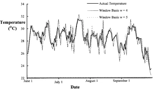
Fig. 6. Curve of the actual temperature and forecasted temperature of Algorithm-B with the window basesw = 4 and w = 5.
Fig. 7. Curve of the actual temperature and forecasted temperature of Algorithm-B with the window basesw = 6 and w = 7.
Based on (13), we can get the fuzzified forecasted variation June 15, 1996 shown as follows: (June 15, 1996)
Step 8) Defuzzify the fuzzified forecasted variations of the main-factor fuzzy time series obtained in Step 7. We use the following combined method to defuzzify the fuzzified forecasted variations:
1) If the grades of membership of the fuzzified forecasted variation are all 0, then we set the forecasted variation to 0.
2) If the maximum membership of the fuzzified forecasted variation occurred at and the midpoint of is , then the forecasted variation is . If the maximum membership of the fuzzified forecasted variation oc-curred at and , and the
mid-points of and are
and , respectively, then the forecasted
vari-ation is [4].
For example, in the above, we can see that the maximum membership value of June 15, 1996 is 0.5 which occurs at and , where the midpoint of is and the midpoint of is . Thus, the forecasted variation of June 15, 1996 is . Step 9) Calculate the forecasted data of the main-factor
fuzzy time series. The forecasted data is equal to the forecasted variation plus the actual data of the last day of the main-factor fuzzy time series. For example, if the forecasted variation of June 15, 1996, is , and the actual daily average temper-ature of June 14, 1996 is 27.5, then the forecasted average temperature of June 15, 1996 is equal to
.
Figs. 1–4 show the forecasting results using Algorithm-A from June 1996 to September 1996, where Algorithm-A only uses one factor (i.e., the daily average temperature) for temper-ature prediction. Figs. 5–8 show the forecasting results using Algorithm-B from June 1996 to September 1996 with different window basis. Table IV shows the forecasting errors of the daily average temperature using Algorithm-A [7] and Algorithm-B with different window bases from June 1996 to September 1996 in Taipei. In general, the forecasting accuracy of the two-factors time-variant fuzzy time series algorithm Algorithm-B is better than the one-factor time-variant fuzzy time series algorithm Al-gorithm-A [7]. In order to further enhance the forecasting accu-racy of the proposed algorithm Algorithm-B, we will modify Al-gorithm-B into AlAl-gorithm-B to further reduce the forecasting errors.
In the following, we will propose the algorithm Algorithm-B based on the concept of -significance level [27], where
, and the repeated transition method, where Algorithm-B is essentially a modification of Algorithm-B.
Definition 3.4: Assume that and are fuzzy time series of the daily average temperature, where is last year's is the data of at date , and is the data of at date . The boundary of ranges from to , where is the boundary length. Then, we can find the
TABLE IV
AVERAGEFORECASTINGERRORS OFALGORITHM-AANDALGORITHM-B WITH
DIFFERENTWINDOWBASES FORTEMPERATUREPREDICTION
TABLE V
DAILYAVERAGETEMPERATURE FROMMAY1995TOOCTOBER1995
INTAIPEI(UNIT: C) [2]
maximum and the minimum of these data. The forecasted temperature of date can not be bigger than and not be smaller than . The algorithm Algorithm-B is now presented as follows:
Algorithm-B :
Step 1) Partition the historical data into suitable groups. Step 2) Compute the variations of the main-factor fuzzy
time series between any two continuous data. Find the maximum decrease and the maximum in-crease , and define the universe of discourse , where and are suitable positive numbers.
Fig. 9. Curve of the actual temperature and forecasted temperature of Algorithm-B with the window basesw = 2 and w = 3.
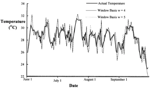
Fig. 10. Curve of the actual temperature and forecasted temperature of Algorithm-B with the window basesw = 4 and w = 5.
Step 3) Partition the universe of discourse into several even length intervals.
Step 4) Define fuzzy sets on the universe of discourse for the main-factor fuzzy time series . Step 5) Define fuzzy sets on the universe of discourse
for the second-factor fuzzy time series . Step 6) Fuzzify the variation of the historical data of the
main-factor fuzzy time series and fuzzify the his-torical data of the second-factor fuzzy time series. Step 7) Choose a suitable window basis . Define the
crite-rion vector , the operation matrix , and the second-factor vector . Then, calculate the fuzzy relationship matrix between the crite-rion vector , the operation matrix , and the second-factor vector. The fuzzified forecasted variation of the main-factor fuzzy time series can be obtained from the fuzzy relationship matrix.
Step 8) Defuzzify the fuzzified forecasted variations of the main-factor obtained in Step 7.
1) Compute the -significance level [27] of the fuzzified forecasted variation as follows:
(16)
where is the fuzzified forecasted varia-tion of date represented by a fuzzy set in the fuzzy time series is the number of elements in the universe of discourse, and
. If , then let ; if
Fig. 11. Curve of the actual temperature and forecasted temperature of Algorithm-B with the window basesw = 6 and w = 7.
Fig. 12. Curve of the actual temperature and forecasted temperature of Algorithm-B with the window basisw = 8.
In this paper, we set the value of the signifi-cance level .
2) If the grades of membership of the -signifi-cance level forecasted variation are all 0, then we set the forecasted variation to 0. 3) If the grades of membership of the
-sig-nificance level forecasted variation
have only one maximum , and the mid-point of is , then the forecasted vari-ation of date is . If the grades of mem-bership of the -significance level forecasted variation have more than one max-imum and , and the midpoints
of and are and
, respectively, then the forecasted
varia-tion of date is .
Step 9) Calculate the forecasted data of the main-factor fuzzy time series. The forecasted data is equal to the forecasted variation plus the actual data of the last day of the main-factor fuzzy time series.
Step 10) Set the boundary length to . Then, we can find the maximum and the minimum among the data from the date of last year to the date of last year. The forecasted temperature of date t obtained in Step 9 can not be bigger than and not be smaller than . If the forecasted temperature is larger than , then we set the forecasted temperature to ; if the forecasted temperature is smaller than , then we set the forecasted temperature to . For example, as-sume that we set the window basis and the boundary length , and we want to fore-cast the temperature of June 6, 1996, in Taipei. Furthermore, assume that the forecasted tempera-ture of June 6, 1996, by using the above steps is 30.0 C. Table V shows the daily average temper-ature from May 1995 to October 1995 in Taipei. The boundary data is from May 27, 1995 to June 16, 1995. According to Table V, we can find that 29.3 C and 24.4 C. Because 30
TABLE VI
COMPARISON OF THEAVERAGEFORECASTINGERRORS OFALGORITHM-A, ALGORITHM-BANDALGORITHM-B TOFORECAST THETEMPERATURE FROMJUNE
1996TOSEPTEMBER1996INTAIPEIWITHDIFFERENTWINDOWBASES
C , we set the forecasted temperature of June 6, 1996, to 29.3 C.
Figs. 9–12 show the forecasting results from June 1996 to September 1996 by using Algorithm-B with different window bases. Table VI shows a comparison of the average forecasting errors of Algorithm-A, Algorithm-B, and Algorithm-B with different window bases. We can see that the forecasting results of Algorithm-B are better than the forecasting results of Al-gorithm-A and Algorithm-B. From Table VI, we can see that when window basis , we almost can get the best fore-casting results, and the forefore-casting results of a smaller window basis are better than the ones of a bigger window basis. This is because the forecasted temperature usually is related to the tem-perature of the recent days. Because the time complexities of the algorithms (i.e., Algorithm-B and Algorithm-B ) are dominated by Step 7, i.e., calculating the fuzzy relationship matrix ,
where as shown in (12) and the
time complexity for calculating is , where is the window basis and is the number of elements in the universe of discourse derived in Step 3 of the proposed algorithms and because there are groups of the historical data derived in Step 1 of the proposed algorithms, the time complexities of the pro-posed algorithms are , respectively.
IV. CONCLUSIONS
In this paper, we have proposed a new fuzzy time series model called the two-factors time-variant fuzzy time series model for handling forecasting problems. Based on the
pro-posed model, we develop two algorithms (i.e., Algorithm-B and Algorithm-B ) for temperature prediction. From Table VI, we can see that the forecasting results of Algorithm-B are better than the forecasting results of Algorithm-A and Algorithm-B. Both of these algorithms have the advantages that they can get good forecasting results. The time complexities of the proposed algorithms are , respectively, where is the number of partitioned groups in the historical data, is the window basis, and is the number of elements in the universe of discourse.
ACKNOWLEDGMENT
The authors would like to thank the referees for providing very helpful comments and suggestions; their insight and com-ments led to a better presentation of the ideas expressed in this paper.
REFERENCES
[1] H. Bentley, “Time series analysis with REVEAL,” Fuzzy Sets Syst., vol. 23, no. 1, pp. 97–118, 1987.
[2] Central Weather Bureau, The Historical Data of the Daily Average
Tem-perature and the Daily Cloud Density Taipei, Taiwan, R.O.C, 1996. (from January 1995 to September 1996).
[3] S. M. Chen, “A new method for forecasting enrollments using fuzzy time series,” in Proc. 1995 National Computer Symp. Chungli, Taoyuan, Taiwan, R.O.C., 1995, pp. 603–609.
[4] , “Forecasting enrollments based on fuzzy time series,” Fuzzy Sets
Syst., vol. 81, no. 3, pp. 311–319, 1996.
[5] M. Y. Day, “Research of Applying Genetic Algorithms to Fuzzy Forecasting—Focus on Sales Forecasting,” M.S. thesis, Tamkang Univ., Taipei, Taiwan, R.O.C., 1995.
[6] J. R. Hwang, S. M. Chen, and C. H. Lee, “A new method for handling forecasting problems based on fuzzy time series,” in Proc. 7th Int. Conf.
Information Management. Chungli, Taoyuan, Taiwan, R.O.C., 1996, pp.
312–321.
[7] , “Handling forecasting problems using fuzzy time series,” Fuzzy
Sets Syst., vol. 100, no. 2, pp. 217–228, 1998.
[8] A. Kandel, Fuzzy Mathematical Techniques with Applica-tions. Reading, MA: Addison-Wesley, 1996.
[9] A. Kaufmann and M. M. Gupta, Fuzzy Mathematical Models in
En-gineering and Management Science. Amsterdam, The Netherlands: North-Holland, 1988.
[10] G. J. Klir and T. A. Folger, Fuzzy Sets, Uncertainty, and
Informa-tion. Englewood Cliffs, NJ: Prentice-Hall, 1988.
[11] G. J. Klir and B. Yuan, Fuzzy Sets and Fuzzy Logic: Theory and
Appli-cations. Englewood Cliffs, NJ: Prentice-Hall, 1995.
[12] K. S. Leung and W. Lam, “Fuzzy concepts in expert systems,” IEEE
Comput., vol. 21, no. 9, pp. 43–56, 1988.
[13] , “A fuzzy expert system shell using both exact and inexact rea-soning,” J. Autom. Reasoning, vol. 5, no. 2, pp. 207–233, 1989. [14] S. Mabuchi, “A proposal for a defuzzification strategy by the concept of
sensitivity analysis,” Fuzzy Sets Syst., vol. 55, no. 1, pp. 1–14, 1993. [15] T. A. Runkler and M. Glesner, “A set of axioms for defuzzification
strategies towards a theory of rational defuzzification operator,” in
Proc. 2nd IEEE Int. Conf. Fuzzy Systems, San Francisco, CA, 1993, pp.
1161–1166.
[16] Q. Song and G. Bortolan, “Some properties of defuzzification neural networks,” Fuzzy Sets Syst., vol. 61, no. 1, pp. 83–89, 1994.
[17] Q. Song and B. S. Chissom, “Fuzzy time series and its models,” Fuzzy
Sets Syst., vol. 54, no. 3, pp. 269–277, 1993.
[18] , “Forecasting enrollments with fuzzy time series—Part I,” Fuzzy
Sets Syst., vol. 54, no. 1, pp. 1–9, 1993.
[19] , “Forecasting enrollments with fuzzy time series—Part II,” Fuzzy
Sets Syst., vol. 62, no. 1, pp. 1–8, 1994.
[20] Q. Song and R. P. Leland, “Adaptive learning defuzzification techniques and applications,” Fuzzy Sets Syst., vol. 81, no. 3, pp. 321–329, 1996. [21] J. Sullivan and W. H. Woodall, “A comparison of fuzzy forecasting and
Markov modeling,” Fuzzy Sets Syst., vol. 64, no. 3, pp. 279–293, 1994. [22] L. X. Wang, A Course in Fuzzy Systems and Control. Englewood
Cliffs, NJ: Prentice-Hall, 1997.
[23] W. Wu, “Fuzzy reasoning and fuzzy relational equations,” Fuzzy Sets
Syst., vol. 20, no. 1, pp. 67–78, 1986.
[24] R. R. Yager, “Implementing fuzzy logic controllers using a neural net-work,” Fuzzy Sets Syst., vol. 48, no. 1, pp. 53–64, 1992.
[25] R. R. Yager and D. Filev, “On the issue of defuzzification and selection based on a fuzzy set,” Fuzzy Sets Syst., vol. 55, no. 3, pp. 255–271, 1993. [26] , “SLIDE: A simple adaptive defuzzification method,” IEEE Trans.
Fuzzy Systems, vol. 1, no. 1, pp. 69–78, 1993.
[27] Y. Yuan and M. J. Shaw, “Induction of fuzzy decision trees,” Fuzzy Sets
Syst., vol. 69, no. 2, pp. 125–139, 1995.
[28] L. A. Zadeh, “Fuzzy sets,” Inform. Contr., vol. 8, pp. 338–353, 1965. [29] , “Outline of a new approach to the analysis of complex system and
decision processes,” IEEE Trans. Syst., Man, Cybern., vol. SMC–3, pp. 28–44, 1973.
[30] , “The concept of a linguistic variable and its application to ap-proximate reasoning, part I–III,” Inform. Sci., vol. 8, 9, pp. 199–249, 301–357, 43–80, 1975.
[31] Z. Li, Z. Chen, and J. Li, “A model of weather forecast by fuzzy grade statistics,” Fuzzy Sets Syst., vol. 26, no. 3, pp. 275–281, 1988.
Shyi-Ming Chen (M'88–SM'96) was born on
Jan-uary 16, 1960, in Taipei, Taiwan, R.O.C. He received the B.S. degree in electronic engineering from Na-tional Taiwan University of Science and Technoilogy, Taipei, in 1992, and the M.S. and Ph.D. degrees in electrical engineering, all from National Taiwan Uni-versity, Taipei, in 1982, 1986, and 1991, respectively. From August 1987 to July 1989 and from August 1990 to July 1991, he was with the Department of Electronic Engineering, Fu-Jen University, Taipei. From August 1991 to July 1996, he was an Associate Professor in the Department of Computer and Information Science, National Chiao Tung University, Hsinchu, Taiwan. From August 1996 to July 1998, he was a Professor in the Department of Computer and Information Science of the same university. Since August 1998, he has been a Professor in the Department of Electronic Engineering, National Taiwan University of Science and Technology. His current research interests include fuzzy systems, database systems, expert systems, and artificial intelligence. He has published more than 100 papers in referred journals and conference proceedings.
Dr. Chen was the winner of the 1994 Outstanding Paper Award of the Journal
of Information and Education and the winner of the 1995 Outstanding Paper
Award of the Computer Society of the R.O.C. He was also the winner of the 1997 Outstanding Youth Electrical Engineer Award of the Chinese Institute of Electrical Engineering, R.O.C, and the Outstanding Paper Award of the 1999 National Computer Symposium, R.O.C. He is a member of the ACM, the In-ternational Fuzzy Systems Association (IFSA), and the Phi Tau Phi Scholastic Honor Society. He is an executive committee member of the Chinese Fuzzy Systems Association (CFSA). He is an executive committee member of the Tai-wanese Association for Artificial Intelligence (TAAI). He is an editor of the Journal of the Chinese Grey System Association. He is listed in International
Who's Who of Professionals, Marquis Who's Who in the World, and Marquis Who's Who in Science and Engineering.
Jeng-Ren Hwang was born on May 4, 1973, in
Tainan, Taiwan, R.O.C.. He received the B.S. degree in computer science from National Tsing Hua University, Hsinchu, Taiwan, in June 1995 and the M.S. degree in the Department of Computer and Information Science at National Chiao Tung University, Hsinchu, in June 1997. His current research interests include fuzzy systems, database systems, and artificial intelligence.