大型貝氏網路推論之時間與準度權衡演算法

(1)

國

立

交

通

大

學

電控工程研究所

碩

士

論

文

大型貝氏網路推論之

時間與準度權衡演算法

A Tractable Time-Precision Tradeoff Algorithm for

Inference in Large-Scale Bayesian Networks

研究生：莊仲翔

指導教授：周志成博士

中

華

民

國

九

十

九

年

七

月

(2)

大型貝氏網路推論之

時間與準度權衡演算法

A Tractable Time-Precision Tradeoff Algorithm for

Inference in Large-Scale Bayesian Networks

研究生：莊仲翔 Student：Chung- Hsiang Chuang

指導教授：周志成 Advisor：Chi-Cheng Jou

國立交通大學

電控工程研究所

碩士論文

A Thesis

Submitted to Department of Electrical and Control Engineering College of Electrical Engineering

National Chiao Tung University in Partial Fulfillment of the Requirements

for the Degree of Master

in

Electrical and Control Engineering July 2010

Hsinchu, Taiwan, Republic of China

(3)

大型貝氏網路推論之

時間與準度權衡演算法

學生：莊仲翔

_指導教授

_：

_周志成

國立交通大學電控工程研究所

摘

要

在不同的領域中，貝氏網路是一種功能強大的分析工具。推論引擎則

是貝氏網路中最重要的部分，負責處理接收到的訊息藉由機率的方式給出

結論。推論引擎可以藉由不同的演算法來實現，並且加速推論的效率。由

於傳統的精確推論演算法在大型貝氏網路中，會大幅降低演算效率導致無

法運作。因此，我們提出了一種新的演算法，稱作 KLA 演算法，來解決在

大型複雜的貝氏網路中推論的問題。KLA 演算法可透過權衡時間和精準度

來提升推論的效率，而且所需要的記憶體空間會是所有推論演算法中最小

的。因此，此演算法能夠更容易的將貝氏網路實現在記憶體受限制的應用

中。為了評估在不同結構下 KLA 演算法的表現，我們設計了一系列的實驗

來觀察準度和計算時間的結果並且和傳統聯結樹演算法來做比較。我們也

將 KLA 演算法運用在現實中的案例上來觀察模擬的成果。

(4)

A Tractable Time-Precision Tradeoff Algorithm for

Inference in Large-Scale Bayesian Networks

Student：Chung- Hsiang Chuang

Advisors：Dr. Chi-Cheng Jou

Department of Electrical and Control Engineering

National Chiao Tung University

ABSTRACT

Bayesian networks (BNs) are powerful tools in diverse fields. The most important part is the inference engine, which draws conclusions by updating probabilities on the basis of the given knowledge. The inference engine can be implemented by using different algorithms, which help BNs draw various conclusions efficiently. Since traditional exact methods collapse when applied to large-scale methods, we propose a new algorithm, called KLA-algorithm, to solve the problem of drawing an inference in a large and complex system. The KLA-algorithm always has tractable computational time and a trade-off with precision. The required memory in KLA-algorithm is the minimum as compared to the other inference algorithms. This advantage extends large-scale BNs to some limited resource applications. In order to verify the KLA-algorithm in a different graph structure, we design a series experiment to compare with the junction tree algorithm and discuss the performance of precision and computation time. We also apply the KLA-algorithm to real-world data in order to carry out some simulations.

(5)

誌

謝

研究這條路，一路走來一直都是跌跌撞撞的，處在迷霧中永遠比撥雲見日的時間還要永久許多。能夠毫無畏懼的一直走到最後是因為有大家一直在旁邊的陪伴。謝謝我的指道教授可以這麼放任的讓我為所欲為，讓我可以做我自己的研究，朝我想走的方向走；即使由於我的固執而走入死路，也會即時指引出另一條可行的道路。然而跟您相處兩年的點點滴滴，您的行事風格，特立獨行的品味對我的影響更甚於課業上的教導。謝謝實驗室的研究同伴們，在苦悶時總是可以一起聊天、吃飯，這一直是我堅持到最後的動力。雖然有時覺得實驗室很吵，但是當實驗室空無一人時，才深深體會到那份吵鬧的珍貴。在我身邊的朋友們，感謝你們的陪伴，大家研究的路都各不相同，但目標都是一致的。彼此的扶持與鼓勵讓我覺得這條旅途並不孤獨。感謝口試委員對論文方面的建議以及提點，與你們討論令我受益良多也讓讓這份作品能更加完整。最後，謝謝我的家人，總是受到你們的呵護與照顧。也在此將這份論文獻給你們。

(6)

A Tractable Time-Precision Tradeoff Algorithm for

Inference in Large-Scale Bayesian Networks

(7)

List of Figures

1.1 Bayesian network modeling a meadow. The structure (nodes and arcs) and

parameters (conditional probabilities table) are shown in the graph. . . 2

2.1 The joint probability P (A, B, C, D, E) can be factorized as the product of all

conditional probabilities, Q P (X|ΠX). . . 8

2.2 (a) Original graph of a multi-connected network. (b) Result draft of original

data output from Phase I and input to Phase II. (c) Result graph after Phase II. The remaining edges are passed from the heuristic (in)dependent test. (d) Result graph output from Phase III. The remaining edges are passed from the exact (in)dependent test, and part of them will be oriented. The result

structure is similar to the original structure. . . 12

3.1 Bayesian network model, structure, and CPTs; here, we parameterize all the

entries in CPT. . . 18

3.2 (a) Original Bayesian network. (b) Corresponding moral graph. The newly

added arcs are shown with dashed lines in the moralized graph. (c) Corre-sponding triangulated graph with two added chords (dashed). (d) Junction tree structure with corresponding cliques and separators. During the mes-sage propagation, mesmes-sages are passed away from clique ACE, beginning with ACE; these message passing route is indicated by the arrows. The numbers

(10)

3.3 Initialization of clique ACE by multiplying the CPT of node C and node E.

The separator CE is initialized to be unity. . . 24

3.4 Part of poly-tree network for each node X with parents U1, ..., UM and children

Y1, ..., YN. . . 26

3.5 (a)G is a moral graph of the Bayesian network and is a union graph in (b).

(b) G is sectioned into four graphs. (c) Junction forest of G, each square

represents a sub-graph in (b) and is called an agent. . . 32

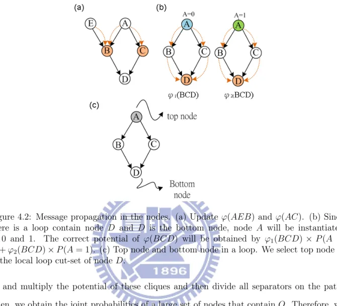
4.1 (a) Simple Bayesian network with a loop. (b) Clique graph from (a); the

parents of node Xi and Xi can be contained in corresponding Ci. (c) Initial

clique potential ϕ(Ci) and separator potential φ(Sj). . . 37

4.2 Message propagation in the nodes. (a) Update ϕ(AEB) and ϕ(AC). (b)

Since there is a loop contain node D and D is the bottom node, node A will be instantiated to 0 and 1. The correct potential of ϕ(BCD) will be obtained

by ϕ1(BCD) × P (A = 0) + ϕ2(BCD) × P (A = 1). (c) Top node and bottom

node in a loop. We select top node A in the local loop cut-set of node D. . 40

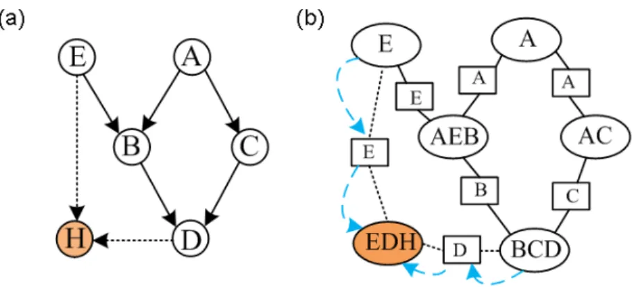
4.3 (a) Addition of a virtual node H, and assigning the interesting set of nodes to

be its parents. (b) Corresponding clique-node EDH. The blue line indicates

the message propagation path, and ϕ(EDH) can be obtained. . . 41

4.4 Propagation path of loopy belief propagation. Blue line represents the

back-ward propagation path. After clique-nodes B, C, D and E have propagated the message to clique-node A, return again until all of clique potentials are

(11)

4.5 (a) Maximum eigenvalue of a structure with ten nodes with different numbers of edges. A greater number of edges will lead to more loops in the structure and a large maximum eigenvalue. The maximum eigenvalue of all the ten nodes is between that of the line structure (the left) and the that of the fully connected structure (the right). (b) Maximum eigenvalue of nine edges with different nodes. A greater number of nodes will lead to simple structures and

the maximum eigenvalue will decrease. . . 46

4.6 Computation time increase exponentially with an increase in the graph

com-plexity. The value on the y-axis is the natural logarithm. . . 47

4.7 (a) Distance level from parents of bottom node X4 to top node X1 of the loop.

(b) KL-divergence between real joint probability and estimated joint

proba-bility of the parents of node X4 in the loop. The estimated joint probability

assumes that the nodes X2 and X3 are independent of each other. The low

value KL-divergence implies that the parents of node X4 are closer to the

in-dependent node. The blue line indicates a loop structure that does not have an outside node, see (a). The green line indicates an outside node added to

parent X3 (shown in (c)) and has less KL-divergence than the blue line. (c)

Addition of an outside node on the left path. . . 49

4.8 Yellow nodes {X1, X2, X3} are the local loop cut-set of node X12. X1 is three

levels from X12, and X2 and X3 are two levels from X12. We can just keep

two levels for approximation, and the reduced local loop cut-set has only two

nodes, {X2, X3}. . . 50

4.9 (a) Poly-tree structure. (b) Multiply networks with few loops. (c) Multiply

networks with many long loops. (d) Multiply networks with many short loops. 52

(12)

5.2 Graph complexity vs. maximum clique size. Size of the clique is represented by the number of nodes in the clique. The maximum clique size grows expo-nentially in junction tree algorithm but fixed in the KLA-algorithm when the

graph complexity increases. . . 55

5.3 Computation time (seconds) of VN-method with different numbers of level

approximations and junction tree algorithm. The computation time is repre-sented in a logarithmic form. Junction tree algorithm lacks one point because the algorithm can not work in the most complex structure (The memory is not sufficient). The VN-method with all levels only has 4 points because the

computation time is intractable in the last three structures. . . 57

5.4 K-L divergence between approximate value and exact value. There is no clear

relation between KL-divergence value and graph complexity. Most K-L

di-vergence values are less than 10−2, which means that we can obtain a good

approximation by the VN-method of the KLA-algorithm. . . 58

5.5 Computation time (seconds) of FB-method with different numbers of level

approximations and junction tree algorithm. The computation time is rep-resented in a logarithmic form. The FB-method when all levels are kept is replaced by that when seven levels are kept here, since the computation time

of keeping all values is always intractable. . . 60

5.6 K-L divergence between approximate value and exact value in FB-method.

There is no clear relation between KL-divergence value and graph complexity, and the K-L divergence in different level approximations are similar. All of

the K-L divergence value are less than 10−2, which means that we can obtain

(13)

5.7 Computational time of different number of evidence nodes in two different methods. The FB-method is presented as diamond with thick line, and the VN-method is circle with thin line. The FB-method has more stable computing

time than VN-method. The y-axis represents the logarithm. . . 63

5.8 Maximum clique of JT and KLA algorithm in different value of threshold

ε2. (a) In 2-bins discretization situation. (b) In 3-bins discretization situation.

Both two situation indicate the JT-algorithm need more large space than

KLA-algorithm. . . 68

5.9 BIC value of the model with different threshold and bins. The blue line is two

bins discretization and the green line is three. The two bins discretization is

always better than three bins. The best network is occur at ε2 = 0.04, with

two bins discretization. . . 69

5.10 BIC value of the model with different threshold ε1. The ε1 value smaller than

0.0016 would have the best structure. . . 70

5.11 Final networks of ozone detection problem. Each circle corresponds a

at-tributes according to the number. The target node is No.73 and only be

connected by Node12 which is wind speed resultant at 11 am. . . 71

5.12 The corresponding precision with different value of vE . The highest precision

is 0.76 and vE is between 0.04 and 0.16. . . 72

5.13 Probability of ozone day on random six days from test-data. The left column is the normal day case and right column is the ozone day case. The dashed

(14)

List of Tables

3.1 X-ray noisy-OR example. The chance that an X-ray (E) will fail to detect two

medical conditions X and Y is just the product of the individual failure chances. 33

5.1 Computation time (seconds) of VN-method with different numbers of level

ap-proximations and junction tree algorithm. The corresponding graph is shown

in Figure 5.3. . . 56

5.2 K-L divergence between approximate value and exact value. NaN represents

that we do not have approximate value. The corresponding graph is shown in

Figure 5.4. . . 58

5.3 Computation time (seconds) of FB-method with different numbers of level

ap-proximations and junction tree algorithm. The corresponding graph is shown

in Figure 5.5. . . 60

5.4 K-L divergence between approximate value and exact value in FB-method.

NaN represents that we do not have approximate value. The corresponding

graph is shown in Figure 5.6. . . 61

5.5 Computational time (sec) of different number of evidence nodes in two different

methods of KLA-Algorithm.The corresponding graph is shown in Figure 5.7. 63

5.6 Seventy-two continuous attributes and one target variable in the data file. . 66

5.7 Precision and cross entropy error of different level approximation. All level is

(15)

Chapter 1 Introduction

1.1 Motivation

Bayesian networks are powerful tools in diverse fields such as medical diagnosis [24], image recognition [1], language comprehension [2], and search algorithms [12]. Bayesian networks are very effective in modeling situations where some information is already known and the incoming data are uncertain or partially unavailable (unlike rule-based or other expert sys-tems, where uncertain or unavailable data lead to ineffective or inaccurate reasoning). These networks also provide consistent semantics for representing causes and effects through an intuitive graphical representation. Because of all of these capabilities, Bayesian networks are being increasingly used in a wide variety of domains where automated reasoning is needed.

The Bayesian network systems can be deconstructed into three components. First is the structure, which represents a set of random variables and their conditional independence. Second is the parameter, which uses a conditional probabilities table to quantify the re-lationship between variables. Third and the most important part is the inference engine, which draws conclusions by updating probabilities on the basis of the given knowledge. The previous two parts can be attained from domain knowledge or by learning from the data. The inference engine can be implemented by using different algorithms, which help Bayesian

(16)

networks draw various conclusions efficiently.

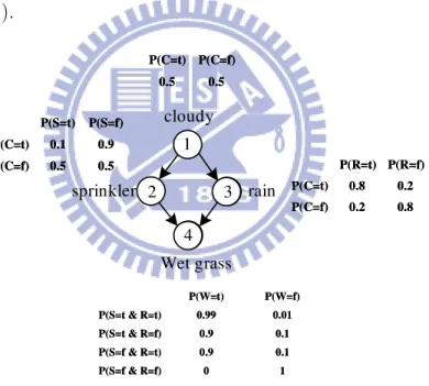
For example, Figure 1.1 shows the simple case for modeling a meadow. The structure, composed of arcs and nodes, indicates the relationship between cloudy weather, sprinkler, rain, and wet grass conditions. The wet grass condition is caused by the rain or the sprinkler condition, and the cloudy weather condition can affect the rain and decide whether the sprinkler should be turned on. The strength of a relationship depends on the conditional probabilities table; these probabilities are deduced on the basis of data or experience. Suppose we observe that the grass is wet in the morning, and wish to know whether it rained or whether the water sprinkler was turned on the previous night. By using the inference engine, the Bayesian network would update the probabilities on the basis of the given information (e.g. the grass is wet.).

1 2 3 4 cloudy rain sprinkler Wet grass 0.5 0.5 P(C=f) P(C=t) 0.5 0.5 P(C=f) P(C=t) 0.8 0.2 P(C=f) 0.2 0.8 P(C=t) P(R=f) P(R=t) 0.8 0.2 P(C=f) 0.2 0.8 P(C=t) P(R=f) P(R=t) 0.5 0.5 P(C=f) 0.9 0.1 P(C=t) P(S=f) P(S=t) 0.5 0.5 P(C=f) 0.9 0.1 P(C=t) P(S=f) P(S=t) 1 0 P(S=f & R=f) 0.1 0.9 P(S=f & R=t) 0.1 0.9 P(S=t & R=f) 0.01 0.99 P(S=t & R=t) P(W=f) P(W=t) 1 0 P(S=f & R=f) 0.1 0.9 P(S=f & R=t) 0.1 0.9 P(S=t & R=f) 0.01 0.99 P(S=t & R=t) P(W=f) P(W=t)

Figure 1.1: Bayesian network modeling a meadow. The structure (nodes and arcs) and parameters (conditional probabilities table) are shown in the graph.

To be considered an expert system, it is important for the system to draw efficient infer-ence. In recent years, several efficient exact inference algorithms have been proposed, and successfully used in different network structures. However, when a system becomes compli-cated and the scale of the network increases, the inference engine requires a large number of computations or a huge amount of memory, and becomes inefficient. In order to solve

(17)

this problem, some people use approximate methods, and others keep improving the exact methods. The approximate methods have a trade-off the between the precision and the com-putational time as well as the memory space. In large-scale networks, the precision is not sufficiently good enough for some applications. On the other hand, there has not been any significant improvement of the exact methods. The most famous method is the multiply sectioned Bayesian network, which divides a network into small sub-networks, and obtains the result by combining the inference in these sub-networks. However, even this method has not efficiently deceased the computation time and memory space required.

In the present exercise, we focus on developing a new algorithm to make the Bayesian networks draw inferences efficiently from complex, large-scale networks. There are three reasons why we pay attention to the problem:

1. A complex large-scale system is commonly used in a variety of fields such as industry, meteorology, and genetics. A Bayesian network is a powerful tool for predictive rea-soning in these fields. Therefore, the above-mentioned problem is very practical in real life.

2. While modeling the large-scale problem, feature selection can be used for simplifying the problem. However, feature selection focuses on the correlation between an input variable and an output variable, but not on the input variables themselves. Therefore, we may lose some information related to the system. Large-scale Bayesian networks can store more information about a system.

3. The memory space is limited in some applications such as embedded system. Therefore, solving this problem is helpful in extending the applications of Bayesian networks to a large scale.

(18)

1.2 Organization

In Chapter 2, we first describe the Bayesian networks, and then present a construction algorithm for large-scale Bayesian networks. In large-scale networks, it is difficult to attain the structure from domain knowledge. Therefore, we briefly discuss the algorithms for obtaining a structure from the data and select the BNPC algorithm [5] to construct our model in Chapter 5.

Chapter 3 presents the parameter learning and inference engine of a Bayesian network. The maximum likelihood method is introduced for estimating the parameters of the model. Two exact inference engines junction tree algorithm [14] and conditioning methods [27] -are described; these -are helpful for the development of our new algorithm in Chapter 4. We also examine the other methods proposed to solve the large-scale networks at the end.

Chapter 4 presents a new algorithm devised by using combination of the two exact

in-ference engines mentioned in Chapter 3. The approximate working of new algorithm is

discussed with respect to obtaining a relatively fast inference. We discuss the complexity of this algorithm and compare this algorithm to other exact inference engines.

In Chapter 5, we first carry out some simulations in order to compare the performance of the new algorithm and the junction tree algorithm for different complexity values of the networks. Next, we apply the new algorithm to real-world data and discuss the result.

(19)

Chapter 2 Large Bayesian Network Structure

Learning

2.1 Introduction

A Bayesian network, also called a belief network, is a graphical structure that allows us to represent and reason an uncertain domain. Formally, Bayesian networks represent a set of random variables and their conditional independence via a directed acyclic graph (DAG). Each node in the graph is associated with a random variable, while the arcs, or directed edges, between the nodes indicate the probabilistic dependencies among the corresponding random variables. For example, a Bayesian network can represent the probabilistic relationships in medical diagnosis. Given the symptoms, the network can be used for computing the probabilities of the presence of various diseases.

The construction of a network structure for a given application by domain experts is a time-consuming task. It is difficult to build a medium-sized network manually. Therefore, one may learn the dependency structure directly from the data via computational methods. Over the last decade, considerable progress has been made with respect to structural learning in Bayesian networks. Two important classes of such algorithms have been defined as the

(20)

based and the constraint-based learning methods [13, 19, 25]. The score-metric-based methods deduce structures by optimizing a scoring function, and the constraint-score-metric-based methods infer structures through conditional independence tests. Since the number of pos-sible network structures grows exponentially with the number of nodes, both methods apply heuristic search in a certain manner.

In a comparative study [17], some currently used structure learning algorithms are iden-tified. One is a method based on a scoring criterion, such as K2 [6] (maximization of the structure probability for the given data), Greedy search [3] (finding the best score of the neighbor and iterate) or SEM [8] (greedy search dealing with missing values). The other is a method based on a constraint-based criterion, such as PC [19] or IC [22] (searching causal-ity using statistical tests to evaluate conditional independence), or BN Power Constructor (BNPC) [5] (using conditional independence tests based on an information theory). However, the problem of learning an optimal Bayesian network from a given data-set is NP-hard [4]. In the present exercise, we have focused on a large, complex system. Therefore, we need a method that can achieve structure learning with limited memory space and tractable time. The best method is BN Power Constructor; however, we still need to modify this method for the construction of our model.

This chapter is organized as follows: Section 2.2 presents the basic concept of Bayesian networks. In Section 2.3, we describe the BNPC structure learning algorithm. Section 2.4 discusses some issues that arise when this algorithm is applied to the construction of a large variable network.

(21)

2.2 Basic Concept of Bayesian Networks

2.2.1 Independence and Conditional Independence

In probability theory, two random variables, X and Y , are said to be independent if

P (X = x, Y = y) = P (X = x)P (Y = y), (2.1)

or equivalently, if

P (X = x|Y = y) = P (X = x), (2.2)

where P (X = x|Y = y) is a conditional probability.

By combining the concept of independent and conditional probability, we can represent the conditional independence as

P (X = x, Y = y|Z = z) = P (X = x|Z = z)P (Y = y|Z = z), (2.3)

or equivalently1,

P (X = x|Y = y, Z = z) = P (X = x|Z = z). (2.4)

In other words, if we know about Z, then X and Y are independent or the knowledge of Y does not help us to guess X when Z is known. We say that X and Y are conditionally independent given Z, and we write this as X⊥Y |Z.

2.2.2 BN Factorization

Suppose that we have a directed acyclic graph (DAG) D with nodes Xi, where i = 1, 2, . . . p.

If there is an arc from node Xi to another node Xj, Xi is called the parent of Xj, and Xj is

a child of Xi. The set of parent nodes of a node Xi is denoted by ΠXi. A directed acyclic

graph is a Bayesian network if the joint distribution of the node values can be written as the

(22)

product of the individual density functions, conditional on their parent variables:

P (X1 = x1, X2 = x2, ..., Xp = xp) =

Y

i

P (Xi = xi|ΠXi = Πxi). (2.5)

where Πxi is the corresponding value of the parent nodes of node Xi .

An example of BN factorization is shown in Figure 2.1. The joint probability P (A, B, C, D, E) is factorized as the product of five conditional probabilities as follows: P (A) · P (B) · P (C|B) · P (D|A, B) · P (D|E).

D

E

C

A

B

P(A) P(B) P(C|B) P(D|E) P(D|A,B)

Figure 2.1: The joint probability P (A, B, C, D, E) can be factorized as the product of all

conditional probabilities, Q P (X|ΠX).

We order all of variables X, such that for any two nodes Xi and Xj, when i < j, there is

a directed path from Xi to Xj. When i < j, Xi is called an ancestor of Xj. The set of all

ancestors of Xj is denoted by an(Xj). On the other hand, Xj is called a descendant of Xi.

The set of all descendants of Xi is denoted by de(Xi). The BN factorization implies the local

Markov property: each variable is conditionally independent of its ancestors given its parent variables,

Xi ⊥ an(Xi)|ΠXi. (2.6)

Recall that the joint distribution can also be calculated from the conditional probabilities using the chain rule as follows:

(23)

P (X1 = x1, X2 = x2, ..., Xp = xp) =

Y

i

P (Xi = xi|Xi−1= xi−1, ..., X1 = x1). (2.7)

By comparing (2.5) and (2.7), we can obtain the following formula:

P (Xi = xi|ΠXi = Πxi) = P (Xi = xi|Xi−1= xi−1, ..., X1 = x1). (2.8)

Because the graph is acyclic, the set of parents is a subset of the set of ancestors, thereby implying the local Markov property.

2.2.3 D-Separation

D-separation provides considerably strong criterion for independence and plays an important role in Bayesian network learning and inference. A path p is said to be d-separated (or blocked) by a set of nodes Z if and only if (at least) one of the following holds:

1. p contains a chain, i → m → j or i ← m ← j, such that the middle node m is in Z. 2. p contains a fork, i ← m → j, such that the middle node m is in Z.

3. p contains an inverted fork (or collider ), i → m ← j, such that the middle node m is not in Z and no descendant of m is in Z.

If every undirected path from a node in Xi to a node in Xj is d-separated by Z, then Xi and

Xj are conditionally independent given Z, in formula form Xi⊥Xj|Z.

For example, in Figure 2.1 we illustrate the following conditional independent relationship using d-separation.

(24)

• (B ⊥ A, C|φ)2_{: B → D ← A is a closed inverted fork path since we do not condition}

on D or it’s descendant E.

• (B ⊥ E|D): B → D → E is a closed chain path since we condition on D.

2.3 BN Power Constructor

The BNPC algorithm was proposed in [5] . The algorithm constructs Bayesian networks by analyzing conditional independence relationships among nodes on the basis of information theory. In information theory, the mutual information (MI) of two random variables is a quantity that measures the mutual dependence of the two variables, defined as

I(Xi, Xj) = X xi,xj P (xi, xj)log P (xi, xj) P (xi)p(xj) ; (2.9)

and conditional mutual information (CMI) is the expected value of the mutual information of two random variables given the value of a third, defined as

I(Xi, Xj|C) = X xi,xj,c P (xi, xj, c)log P (xi, xj|c) P (xi|c)p(xj|c) . (2.10)

In this algorithm, the conditional mutual information is used as conditional independent

tests. When I(Xi, Xj|C) is smaller than a certain threshold value ε, we say that Xi, and Xj

are d-separated by the condition-set C, and are conditionally independent.

The entire procedure of this algorithm can be decomposed into three phases as follows: PhaseI: (Drafting)

In the first phase, the algorithm computes the mutual information of each pair of nodes as a measure of closeness, and creates a draft on the basis of this information. We select the MI of the pairs of nodes that are greater than a threshold ε, and order them from large to

(25)

small. Then beginning from the large, we place an edge between the corresponding pair of nodes if there is no path between these nodes. After at most (n − 1) edges are drafted (n is the number of nodes in the graph), we obtain a draft of the structure. This phase ensures that the output draft is a single-connected structure. In fact, if the original graph is just a single-connected graph, the draft would be the same as the original one. The draft created in this phase is the base for the next phase.

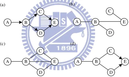
We use the same simple multi-connected network example as that in [5]. Suppose we have a database of the original Bayesian networks, as shown in Figure 2.2(a). The task is to recover the original networks from the data. Suppose we have I(B, D) ≥ I(C, E) ≥ I(B, E) ≥ I(A, B) ≥ I(B, C) ≥ I(C, D) ≥ I(D, E) ≥ I(A, D) ≥ I(A, E) ≥ I(A, C), and all mutual information is greater than ε, the draft obtained from Phase I is shown in Figure 2.2(b).

PhaseII: (Thickening)

In the second phase, the algorithm adds edges when the pairs of nodes are not conditionally independent of a certain conditioning set. We examine all pairs of nodes that have mutual information greater than ε and are not directly connected. An edge is added only when two nodes are not independent given a certain condition-set. The condition-set can be found by using a heuristic method, and hence, it may not be able to find the correct condition-set for a special group of structures and has some edges that are wrongly added in this phase.

For example, the graph after Phase II is shown in 2.2(c). An edge such as [AC], [AD], [CD], or [AE], is not added because the CI test can reveal that these pairs of nodes are independent of the given corresponding condition-set.

PhaseIII: (Thinning)

In the final phase, each edge is examined using conditional independence tests and will be removed if the two nodes of the edge are conditionally independent. Since Phase II has some incorrectly added edges, we check the edges again in this phase. In order to guarantee a

(26)

correct structure, we use a correct procedure to find the exact condition-set. After obtaining the correct structure, we use the algorithm to orient some of the edges.

The correct procedure for finding the condition-set can replace the heuristic procedure in Phase II. However, in practice, the heuristic procedure usually uses relatively few conditional independent tests and requires a relatively small condition-set. Therefore, in order to speed up the algorithm, the correct procedure is used only in the final phase.

The graph after the completion of Phase III in our example is shown in Figure 2.2(d); this graph has the almost same structure as that of the original graph. Edge [BE] is removed since B and E are independent given the condition-set {C, D}. In this graph, we can only orient two edges [CE] and [DE]; the reason for this will be described in Section 2.4.2.

B D C E A (a) B D C E A (b) B D C E A (c) B D C E A (d)

Figure 2.2: (a) Original graph of a multi-connected network. (b) Result draft of original data output from Phase I and input to Phase II. (c) Result graph after Phase II. The remaining edges are passed from the heuristic (in)dependent test. (d) Result graph output from Phase III. The remaining edges are passed from the exact (in)dependent test, and part of them will be oriented. The result structure is similar to the original structure.

(27)

2.4 Issues Related to BN Power Constructor

2.4.1 Threshold Selection

The threshold has an effect on two places in the algorithm. One is in phase I, when we

choose the MI of the pairs of nodes which are greater than a threshold ε1. The other is

in Phase II and III, the procedure of testing the conditional independence of the pairs of

nodes. If I(Xi, Xj|C) is smaller than a threshold value ε2, then Xi and Xj are conditionally

independent. When ε1 is large, the small edges would be considered; the small edges are set

for the conditional independent test. However, the graph would be too simple to explain the

data. On the other hand, if ε1 is small, many edges will be examined. We will be able to

determine a relatively more correct structure, but waste more time in computation. For the

threshold value ε2 of the conditional independent test, the large ε2 leads to the omission of

a considerable number of edges, and the graph structure will be too simple. However, the

small value of ε2 will lead to a complex graph, and cannot explain the data well.

In practice, the optimal threshold is unknown beforehand. Moreover, the optimal thresh-old is problem and data-driven, i.e., it depends, on one hand, on the database and its size and, on the other hand, on the variables and the numbers of their states. Therefore, it is not possible to set a default threshold value that will accurately determine conditional indepen-dence while using any database or problem. Therefore, we would score structures learned using different thresholds by a likelihood-based criterion evaluated using the training set and select the threshold leading to the structure achieving the highest score. The most commonly used scoring function is the Bayesian information criteria (BIC) which is derived on the basis of the principles stated in [23]. The BIC is a criterion for model selection among a class of parametric models with different numbers of parameters and has the following formulation:

BIC(G, D) = logP (D|G, θM L) −1

(28)

where D is the data-set, M L are the parameter values obtained by likelihood maximization, and the network dimension Dim(G) is used for preventing the graph from becoming very over-fitting. The other methods such as test error are also a good pointer.

2.4.2 Orientation Problem

In the last phase of the BNPC algorithm, we orient the edges in the final step. The procedure involves the identification of colliders, as the other edge orientations are virtually based on these identified colliders. Colliders can be found by a conditional independence test. For

any two nodes Xi and Xj that are not directly adjoined and are dependent according to the

smallest given condition-set C , by d-separation, we can say that nodes Xi and Xj are the

parents of the node set C, i.e., Xi → C ← Xj.

However, in practice, we cannot always orient all the edges. In a special case, if a part of the structure is a line structure, which means that the nodes adjoin each other one by one, then there are no identifiable collides. Therefore, we cannot know the exact direction of the structure. For example, in Figure 2.2(d), we can only identity the collider E; C and D are the parents of E. The other edges cannot be oriented since we do not have any further information.

Therefore, expert knowledge is required in this situation. In the worst case, there is no expert knowledge and we cannot orient all the edges. We will arbitrarily assign the variable order in this case, and the previous order will be the ancestors of the reverse order. Therefore, the directed graph cannot explain a causal relationship between two connected nodes, but just a conditional relationship between them.

(29)

Chapter 3 Bayesian Network Inference

3.1 Introduction

In the previous chapter, we described an algorithm for building a Bayesian network struc-ture. In this chapter, our goal is to draw conclusions when new information, or evidence, is observed. For example, in the field of meteorology, the objective of a meteorological sys-tem is to forecast weather with some observed climate data (e.g., sys-temperature, cloud, and humidity data). The mechanism of drawing conclusions in Bayesian networks is called an in-ference engine, or the propagation of evidence. The inin-ference engine consists of updating the probability distributions of variables (e.g., weather forecast) according to the newly available evidence (e.g., climate data).

Two types of algorithms for an inference engine are available, namely, exact and ap-proximate. The basic concept of an exact inference is based on the Bayesian theorem. In accordance with the variable dependency relationships residing in a network, we can use more efficient methods to update probabilities. In recent years, several efficient methods have been developed, such as variable elimination [29], junction tree, and belief propagation [20]. However, all the exact algorithms suffer from a combinatorial explosion when dealing with large and complex networks.

(30)

Approximate inference methods are used in large-scale systems when exact methods are computationally inefficient. The basic idea of an approximate inference is to generate a sam-ple from the joint probability distribution of the variables, and then use the generated samsam-ple to compute approximate values for the probabilities of certain events given the evidence. Dif-ferent approximate methods attempt to improve the quality or efficiency of approximations. The problem with an approximate inference is the requirement of an adequate sample size. In large systems, large amounts of data are required to ensure reasonable results.

Although approximate methods can handle large-scale systems, for obtaining a better inference result, exact methods are used. We have reason to believe that the exact methods can be improved to be efficient while dealing with large, complex systems. Therefore, in the present exercise, we will also focus on the exact inference algorithms in this chapter.

This chapter is organized as follows: Section 3.2 presents an approach for estimating the parameters of Bayesian networks. After both the structure and the parameters are provided, the inference engine can be launched. In Section 3.3, the exact inference algorithms used for Bayesian networks are considered. The exact inference algorithms that we consider include the junction tree algorithm and belief propagation algorithm. Both algorithms will be used for developing a new algorithm in the next chapter. Section 3.4 discusses the advantages and the shortcomings of both the algorithms and explains why we need to develop a new algorithm for Bayesian networks.

3.2 Parameter Learning

Before trying to launch the Bayesian network (BN) inference engine, we have to specify the BN completely. There are two major parts for learning a BN from data, one is the structure learning, and the other is the parameter leaning. In Chapter 2, we described a structure learning method. Once the structure of a BN is determined, the problem left is to learn the parameters from the data.

(31)

We take a standard statistical modeling approach for parameter learning. The distri-bution of the data is unknown, but is assumed to belong to some given family of possible distributions. We label the distinct members of the family by the value of a set of

parame-ters θ = (θ1, ..., θM)T. Thus, θ determines the unknown probabilities, and our task is to use

the data to estimate θ. There are many statistical methods for doing so. Here, we adopt the maximum likelihood estimation method. In the following paragraphs, we discuss how to parameterize the Bayesian networks by θ and use the maximum likelihood approach for estimating the optimal values of θ.

3.2.1 Bayesian Networks Model Parameterization

Suppose that we have a directed acyclic network (DAG) D with nodes Xi, where i =

1, 2, . . . , p. We use capital letters, such as X, Y , and Z, as variable names and lowercase letters, x, y, and z, to denote the specific values taken by these variables. Sets of variables are denoted by boldface capital letters X, Y , and Z, and the assignments of values to the

variables in these sets are denoted by boldface lowercase letters, x, y, and z. Let ΠXi denote

the set of parent nodes of Xi in D. If Xi does not have a parent, ΠXi is the empty set. A

particular value in the joint distribution is represented by P (X1 = x1, X2 = x2, . . . , Xp = xp),

or more compactly, P (x1, x2, . . . , xp). We can factorize (Section 2.2.2) the joint probabilities

as:

P (x1, x2, . . . , xp) =

Y

i

P (xi|Πxi). (3.1)

Therefore, a Bayesian network can be parameterized using a vector of conditional probability table (CPT) entries, one entry for each value of each node and each instantiation of the parents of the nodes. We now define the overall parameter θ, which is composed by parameter

θxi|Π_xi to represent the conditional probability table entry P (xi|Πxi) for each possible value

(32)

Now, (2.7) becomes

P (x1, x2, . . . xp|θ) =

Y

i

P (xi|Πxi, θxi|Π_xi). (3.2)

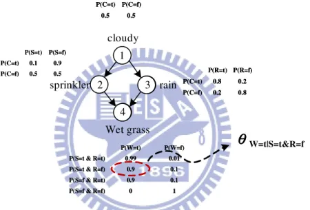
For example, in graph 3.1, we show a simple Bayesian network with structure and four

conditional probability tables (CPTs) for each node. θxi|Πxirepresents each conditional

prob-ability in CPT, such as θW =T |S=T ,R=F = P (W et(W ) = T |Sprinkler(S) = T &Rain(R) =

F ) = 0.9. 1 2 3 4 cloudy rain sprinkler Wet grass 0.5 0.5 P(C=f) P(C=t) 0.5 0.5 P(C=f) P(C=t) 0.8 0.2 P(C=f) 0.2 0.8 P(C=t) P(R=f) P(R=t) 0.8 0.2 P(C=f) 0.2 0.8 P(C=t) P(R=f) P(R=t) 0.5 0.5 P(C=f) 0.9 0.1 P(C=t) P(S=f) P(S=t) 0.5 0.5 P(C=f) 0.9 0.1 P(C=t) P(S=f) P(S=t) 1 0 P(S=f & R=f) 0.1 0.9 P(S=f & R=t) 0.1 0.9 P(S=t & R=f) 0.01 0.99 P(S=t & R=t) P(W=f) P(W=t) 1 0 P(S=f & R=f) 0.1 0.9 P(S=f & R=t) 0.1 0.9 P(S=t & R=f) 0.01 0.99 P(S=t & R=t) P(W=f) P(W=t)

Ӱ

W=t|S=t&R=f

Figure 3.1: Bayesian network model, structure, and CPTs; here, we parameterize all the entries in CPT.

3.2.2 Maximum Likelihood with Complete Data

Maximum likelihood estimation (MLE) is a popular statistical method used for fitting a statistical model to data, and providing estimates for the parameters of the model (i.e., the probability of the observed data as a function of the unknown parameters). This procedure involves the calculation of the likelihood on the basis of the data according to the model, and finding the values of the parameters that maximize this likelihood. For complete data with no constraints related to the component parameters, the calculation of the maximum likelihood is divided into a collection of local calculations, as we shall see.

(33)

For discrete Bayesian networks, suppose that we have a sample of N independent and

identically distributed cases d = {x(1), ..., x(n)}, where x(n)_{= (x}(n)

1 , ..., x (n)

p ). The likelihood is

a function of the parameters that is proportional to the probability of the observed data:

P (d|θ) =

N

Y

n=1

P (x(n)|θ). (3.3)

We assume that the parameters are unknown and estimate them from data. We focus on the problem of estimating a single setting of the parameters that maximizes the likelihood (3.3). Equivalently, we can maximize the log likelihood:

L(θ) = log P (d|θ) = N X n=1 log p(x(n)|θ) = N X n=1 p X i=1 log p(x(n)_i |Π_x(n) i , θ_x(n) i |Π_x(n) i ) (3.4)

where the last equality makes use of the factorization (2.7). Let NX(x) be the number of

occurrences in the data set where X = x. (3.4) can be rewritten as:

L(θxi|Π_xi) = X i X xi,Π_xi N (xi, Πxi)log(θxi|Π_xi) (3.5)

The problem of maximizing the data log-likelihood subject to the parameters can be restated as: max L(θxi|Π_xi) = X i X xi,Πxi N (xi, Πxi)log(θxi|Π_xi) subject to X xi θxi|Π_xi = 1.

This is a simple optimal problem. We just need to solve the following equation:

∂L ∂θxi|Π_xi

= N (xi, Πxi)

θxi|Π_xi

(34)

where λ is the Lagrange multiplier. After computation, we obtain θxi|Πxi = −N (xi, Πxi)/λ.

SinceP

xi

θxi|Π_xi = 1, the solution of λ is −N (Πxi), where N (Πxi) =

P xi N (xi, Πxi).Therefore , θxi|Π_xi = N (xi, Πxi) N (Πxi) (3.7)

In other words, on the basis of a database of cases, for all nodes Xi, the conditional

proba-bilities are estimated by using the ratio of the corresponding counts.

There are other issues in parameter learning, such as dealing with incomplete data, and updating the parameter on-line. Many approaches to obtain better parameters on different situations have been reported. However, in this present exercise, we just pay attention to the complete data parameter learning.

3.3 Inference engine

The inference engine is the core of the Bayesian networks. Only by an inference engine, a BN can work as an expert system to predict, diagnose, or detect fraud. We can think of the inference engine as a human brain, which uses the past experience (i.e., CPT) to answer questions in new situations (i.e., given evidence). Like a human brain, an efficient and general inference engine leads to versatile applications of a BN.

With respect to loops, there are two different types of directed graphs, namely, single-connected networks and multiple-single-connected networks. The single-single-connected network, also called a poly-tree, is a directed graph without loops, or for any two nodes in the graph, there is only one path between them. It is straightforward to develop propagation algorithms on poly-trees, but poly-trees are not suitable in many real-world problems due to its oversimplified structures. The multiple-connected network is a directed graph containing loops and is thus adequate for real-world situations. In order to propagate information in a multiple-connected network, the commonly used approach is to transform the multiple-connected structure into a single-connected network.

(35)

Both conditioning and clustering inference methods are widely used in single-connected and multiple-connected networks. Conditioning methods involve the breaking of the commu-nication pathways along the loops by instantiating a select group of variables. This results in a single-connected network in which poly-tree propagation algorithms can be applied. For either a single-connected or a multiple-connected network, clustering methods build an asso-ciated graph in which each node corresponds to a set of variables. This leads to a network with poly-trees.

In the following paragraphs, we discuss two algorithms: conditioning algorithm (condi-tioning method) and junction tree algorithm (clustering method).

3.3.1 Junction Tree Algorithm

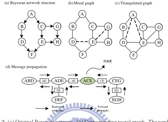
The idea of the junction tree algorithm is to aggregate nodes into a set of nodes, called cliques, which result in a local structure called a junction tree devised for propagating the evidence in the network. The algorithm has five steps, namely, moralization, triangulation, constructing the junction tree, updating the potentials, and propagation.

The junction tree algorithm can be described as follows: Moralization:

For a directed acyclic graph, the corresponding moral graph is formed by connecting the parents of each node, and then making all edges in the graph undirected. In a moral graph, nodes with a common child are said to be married and thus form a family.

In this step, the BN graph (directed acyclic graph) is transformed into an undirected

graph. The moral graph Gm is obtained by linking the parents of each node and dropping

the directions in the original BN graph D. The goal is to combine the family of nodes, since the family members contain of the conditional probability. An example of the moralization is shown in Figure 3.2(b).

Triangulation:

(36)

A B C D F G H E A B C D F G H E A B C D F G H E

ABD ADE ACE CEG

DEF EGH AD DE AE CE EG 1 3 5 2 4 8 6 9 1 0 7 root Backward propagate Forward propagate

(a) Bayesian network structure (b) Moral graph (c) Triangulated graph

(d) Message propagation

Figure 3.2: (a) Original Bayesian network. (b) Corresponding moral graph. The newly added arcs are shown with dashed lines in the moralized graph. (c) Corresponding triangulated

graph with two added chords (dashed). (d) Junction tree structure with corresponding

cliques and separators. During the message propagation, messages are passed away from clique ACE, beginning with ACE; these message passing route is indicated by the arrows. The numbers indicate a possible message passing order.

an edge joining two nodes that are not adjacent in the cycle. Because any chord-less cycle has at most three nodes, chordal graphs are also called triangulated graphs. A specific moral graph can have many different triangulated graphs. Several triangulation methods have been proposed, but none of them guarantee the generation of the minimum added chords. Note that it is NP-hard to find the minimum added chords. The triangulated graph is shown in Figure 3.2(c).

Construction of junction tree:

A junction tree is a mapping of a triangulated graph into a tree that can be used for speeding up the message propagation in the graph. An intermediate result of the process is called a clique graph. The basic operating unit or node in a junction tree is called a clique, formed by the maximum set of fully-connected nodes in a triangulated graph. In a clique

(37)

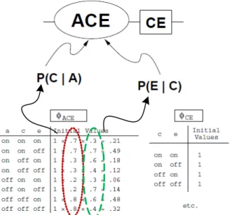
graph, each clique-node corresponds to a clique, and two clique-nodes are connected by an edge if they have a common node in the graph. A junction tree is then constructed by forming a maximal spanning tree from the clique graph. A spanning tree of the undirected graph is a sub-graph that is a tree and connects all the vertexes. We assign the intersection of the adjacent nodes as a weight to each edge, and use this to assign a weight to a spanning tree by computing the sum of the weights of the edges in that spanning tree. The maximal spanning tree is then a spanning tree with a weight that is greater than or equal to the weight of every other spanning tree. Each edge on the junction tree has an attached separator consisting of the intersection of the adjacent clique-nodes. The junction tree structure is shown in Figure 3.2(d). We see that the cliques of the triangulated graph are EGH, CEG, DEF , ACE, ABD, and ADE, which are the ellipse shown in Figure 3.2(d), and the corresponding separator is shown in the square.

Transfer of potentials:

For each clique Ci and separator Si, we define a non-negative potential ϕ(Ci) and φ(Si),

respectively. A potential is actually a table, which eventually represents a joint probability

distribution of the corresponding nodes. Both ϕ(Ci) and ϕ(Si) are initialized to be unity.

For each node X of the original Bayesian network, we choose one clique Ci that contains X

and all parents of X, and then multiply the CPT of X with ϕ(Ci). Figure 3.3 illustrates

the initialization procedure on the potential tables of clique ACE and separator CE. In this example, node C and node E are assigned to clique ACE, but not node A. Therefore, after initialization, ϕ(ACE) = P (C|A)P (E|A), and ϕ(CE) = 1.

(38)

Figure 3.3: Initialization of clique ACE by multiplying the CPT of node C and node E. The separator CE is initialized to be unity.

Propagation:

After initializing the junction tree potentials, we now perform global propagation in order to make these potentials locally consistent. Global propagation consists of a series of local manipulations, called message passes, that occur between a clique X and a neighboring clique Y . A message pass from X to Y forces the belief potential of the intervening separator to be consistent with ϕ(X). Before the propagation begins, the graph is orientated by designating one node as the root; any non-root node that is joined to only one other node is called a leaf. In the first step, messages are passed inwards: starting at the leaves, each node passes a message along the (unique) edge towards the root node. The junction tree structure guarantees that it is possible to obtain messages from all other adjoining nodes before passing the message on. This continues until the root has obtained messages from all of its adjoining nodes. The second step involves passing the messages back out: starting at the root, messages are passed in the reverse direction. The execution of the algorithm is complete when all leaves have received their messages, as shown in Figure 3.2(d). The message propagation between two nodes in a junction tree can be shown as follows:

(39)

a. First, update the separator potential.

φ∗(S) =X

V /S

ϕ(V ). (3.8)

b. Next, update the clique potential

ϕ∗(W ) = ϕ(W ) · φ∗(S)/φ(S). (3.9)

Once the algorithm is terminated, the clique potentials and separator potentials are the joint probabilities of the nodes in the clique.

The second part of propagation is the situation of the given evidence. We only keep the evidence state of nodes in the corresponding cliques, and replace the other state values with zero; we then perform the message propagation again. Upon completion, the clique potentials and separator potentials are proportional to the joint probabilities of the nodes in the clique. We just need to normalize the potential, the correct joint probabilities will then be obtained. There are two problems related to the junction tree algorithm. First, the optimal result of the triangulation is NP-complete. Second, the size of the cliques can be prohibitive, in terms of memory requirements as well as the computational cost of the propagation. Each message-passing step requires marginalization, which, for the case of tabular CPTs, is exponential with respect to the size of the largest clique. Therefore, in the case of a large-scale or complex system, this algorithm is inefficient.

3.3.2 Conditioning Algorithm

Before we describe the conditioning algorithm, we will review Pearl’s poly-tree algorithm, which is one of the methods used for message propagation and will be used in the conditional algorithm. Pearl’s algorithm for computing the posterior of any variable in a belief network (without loops) exploits the fact that each variable X separates the belief network into two disjoint parts, one above X, and the other below X. This algorithm denotes four elements

(40)

in the propagation procedure. The predictive messages πU,X which are passed down from

each parent U of X, and the likelihood messages λY,X which are passed up from each child

Y of X. These message are combined to yield the predictive support πX, and the likelihood

support λX. The posterior for X is obtained by normalizing the product of πX and λX.

Pearl’s algorithm is defined by these four elements as follows:

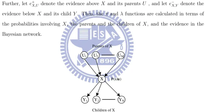
Suppose a given node X having parents U1, ..., Um and children Y1, ..., Yn, as shown in

Figure 3.4. P (x|u1, ..., um) is a shorthand for CPT of each node X P (X = x|U1 = u1, ..., Um =

um). Evidence is represented with E, with evidence above X (evidence at the ancestors of

X) written as e+_X and evidence below X (evidence at the descendants of X) written as e−_X.

Further, let e+_X,U denote the evidence above X and its parents U , and let e−_X,Y denote the

evidence below X and its child Y . Then, the π and λ functions are calculated in terms of the probabilities involving X, the parents and the children of X, and the evidence in the Bayesian network. X U1 U2 UM Y1 Y2 YN Parents of X Children of X P(x|u)

Figure 3.4: Part of poly-tree network for each node X with parents U1, ..., UM and children

Y1, ..., YN.

1. Posterior for variable X:

PX|e(x) ∝ πX(x)λX(x). (3.10)

(41)

πX(x) = PX|e+_X(x) = X u1,...,um P (x|u1, ..., um) · Y i πUi,X(ui). (3.11)

3. Likelihood support for X:

λX(x) ∝ P_e− X|X(x) = n Y j=1 λYj,X(x). (3.12)

4. Predictive message sent to child Yk:

πX,Yk(x) = PX|e\e−_X,Y(x) ∝ πX(x) n

Y

j=1,j6=k

λYj,X(x) (3.13)

5. Likelihood message sent to parent Uk:

λX,Uk(uk) = Pe\e−_X,Uk|Uk(uk)

= X x X u1,...,um λ(x)P (x|u1, ..., um) Y j=1,j6=k πUj,X(uj). (3.14)

The details of these formulas are not as important to our discussion as to the understanding of the conditional algorithm. In conclusion, Pearl’s algorithm is similar to the classic forward-backward algorithm for information sharing. The posterior for each node depends on the message sent to it by its parents and children, if any. For a more in-depth review of the belief algorithm, please refer to [15].

When the network is not singly-connected, we introduce the notion of conditioning in order to apply the poly-tree algorithm. In the method of conditioning, a set of nodes called a loop cut-set break the dependency loops in a belief network, so named because its members

(42)

are selected such that every loop (a minimal multiply connected subset of the network) is cut by at least one member of the set. After the loop cut-set identified, the conditioning algorithm requires the instantiation of the members of the cut-set. Combinations of the instantiations of the loop-cut-set nodes are the instances of the cut-set. In the context of some observed evidence, the instances are solved with an efficient method for solving single-connected networks. We apply Pearl’s algorithm for solving the single-single-connected networks. For single-connected networks, this algorithm is linear with respect to the size of the network. Finally, in the method of conditioning, the answers of the single-connected sub-problems are combined to calculate the final probability of interest.

The following are the main steps of the conditioning algorithm:

Suppose a multiply connected network D with a loop cut-set C = {C1, ..., Cm} and

evidence node E = e. For any given node X, the method of conditioning calls for the propagation of this evidence in each instance in order to calculate the updated posterior

probabilities for the node X of the network. We associate with each unique instance c1, ..., cm

an integer label i, and denote P (c1, ..., cm) as the weight of the instance wi.

• In the first step, the weights for all instances are calculated and stored during the initialization of the priors in the network. Therefore,

wi = P (c1, ..., cm) = P (c1)P (c2|c1)...P (cm|c1, ..., cm−1). (3.15)

If we observe the value e of node E, then we calculate the new weight, w_i∗, of instance

i as follows:

w_i∗ = P (c1, ..., cm|e) = αP (e|c1, ..., cm)P (c1, .., cm) = αP (e|instance i) × wi, (3.16)

where α = _{P (e)}1 , obtained by normalizing the new weights.

(43)

for each cut-set instance, given the values assigned to the loop-cut-set nodes in that instance and evidence e. We apply Pearl’s algorithm for propagating the evidence in a single-connected network to solve each instance. For each instance i, we assign a probability to each value x of node X,

P (x|e, instance i) = p(x|e, c1, ..., cm). (3.17)

• In the final step, we simply sum the belief over all instances, weighted by the likelihood of the instances: P (x|e) = X c1,..,cm P (x|e, c1, ..., cm)p(c1, ..., cm|e) = X i P (x|e, instance i) × w∗_i. (3.18)

For additional evidence, we repeat this procedure each time by multiplying the old weight assigned to an instance with the probability of the observed value given that instance. There-fore, the method of conditioning provides a mechanism for performing a general probabilistic inference in multiply connected belief networks.

3.4 Why New Algorithm?

3.4.1 Exact Algorithm Problem

In the previous section, we described two exact inference algorithms: junction tree algorithm and conditioning algorithm. In the case of the junction tree algorithm, we might have to spend a considerable amount of time on building the junction tree. In the triangulation step, finding the best elimination order is NP-hard. If we arbitrarily assign the order, we may add many unnecessary fill-in edges, which would lead to large cliques. There are two problems when the clique of a junction tree is large. First, the potential table is huge and grows exponentially with respect to the size of clique. For example, suppose we have 20 nodes in a

(44)

clique, and each node has two statuses, then the potential table has 220 entries, which need

220× 32 memory; 32 is the number of bits required by a float value. If there are 25 nodes

in the clique, we may need approximate 1 − GB memory to store the data. Not to mention there are always more than two statuses of the nodes. In general, the limited memory of Matlab is 2 GB∼ 3 GB, the same as that of other program platforms. Further, there will be more problems if the algorithm is applied to embedded systems, which always have less memory than a PC. Maybe in the future, we will not be restricted by this problem, but now, this is an obstacle that we have to face. The other problem is that the computational time increases exponentially. In the case of a propagation, we have to calculate the potential of the separators and the cliques. If a clique is large, we need to perform a significantly high number of summations in order to obtain the marginal potential, which will waste a considerable amount of time. Therefore, there are some obstacles when the junction tree is implemented in large-scale networks.

In the case of a conditioning algorithm, unlike in the case of the junction tree algorithm, we preserve the original structure since no new edges are added. Therefore, only CPTs need be stored in the memory for computing the probabilities. However, in a multiple-connected structure, the computation of probabilities is very redundant. We need to calculate three different types of probabilities in order to obtain the marginal probabilities of the nodes given the evidence (See (3.15) to (3.18)). Further, when the loop-cut-set is large, the computation complexity increases exponentially. Finding the minimum loop cut-set is also an NP-hard problem. Therefore, this algorithm is also inappropriate for implementation in the large-scale networks because of the computational inefficiency.

3.4.2 Some Approaches for Large-Scale Inference

Since both exact methods collapse when applied to large-scale methods, how do we draw inference in large, complex systems? There are three main methods have been proposed for application to large systems, namely, multiply sectioned Bayesian networks [28], noisy

(45)

Or-gate models [26], and hybrid inference methods [7]. In the following paragraphs, we will briefly introduce and discuss these methods.

Multiply sectioned Bayesian networks (MSBNs)

A multiply sectioned Bayesian network is an extension of the Bayesian network model for the support of flexible modeling in large and complex problem domains. An MSBN consists of a set of interrelated Bayesian sub-nets, each of which encodes an agent’s knowledge concerning a sub-domain. Global consistency among sub-nets in an MSBN is achieved by communication. Once the information for all the agents is updated, we obtain complete knowledge of the system. For example, in the field of medical science, we can separate the physical structure of the body into different parts, such as brain, respiratory system,

and gastrointestinal system. All of them have different but related knowledge domains.

Therefore, we have several different types of doctors, who check their professional parts, and by communicating other domain knowledge to diagnose the disease. Therefore, we do not require to draw an inference in a large-scale system, but only an inference in some small sectioned networks.

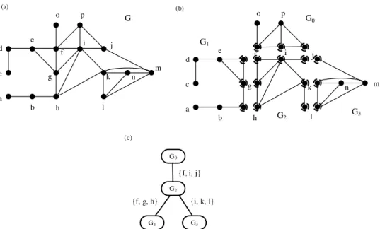
The inference method is called a junction forest algorithm (see Figure 3.5). It is similar to a two-layered junction tree. The first layer is in the sectioned networks. For each agent, we construct a little junction tree to draw the inference. The second layer is on an agent. We view each agent as a supper clique and build a junction tree again to communicate with each other. Since all sectioned networks are small, we can efficiently construct a junction tree and draw an inference. Therefore, we can efficiently handle the large-scale problem.

(46)

(a) d c a b h l m n k j p o f i g e (b) p o m n d c a b g e h l k j f i G G1 G0 G2 G3 (c) G0 G2 G1 G3 {f, i, j} {i, k, l} {f, g, h}

Figure 3.5: (a)G is a moral graph of the Bayesian network and is a union graph in (b). (b) G is sectioned into four graphs. (c) Junction forest of G, each square represents a sub-graph in (b) and is called an agent.

Noisy Or-gate model

Recall that Bayesian Networks require the condition probabilities of each variable given all combination of the values of its parents. Therefore, if each variable has only two states

and a variable has p parents, we must specify 2p _{conditional probabilities for that variable.}

When p is large, the storage requirements as well as the inference algorithm computations become infeasible.

The idea of noisy Or-gate methods is attempt to avoid specifying every entry in the con-ditional probability table. In other words, we assume each parent causes child to contribute independently. Thus, the probability that parents have an effect on a child is simply the product of the probabilities of the effect of each parent.

As a simple example, medical causal models commonly assume that all the possible causes of a symptom act independently. The person who either tuberculosis (X) or cystic fibrosis (Y ) will have a normal lung X-ray (E). Further, tuberculosis has a failure rate of 70% with respect to showing up on an X-ray, and cystic fibrosis has a corresponding failure rate of 40%. The noisy-OR model states that if someone has both tuberculosis and cystic fibrosis,

大型貝氏網路推論之時間與準度權衡演算法

國

立

交

通

大

學

電控工程研究所

碩

碩

碩

碩

士

士

士

士

論

論

論

論

文

文

文

文

大型貝氏網路推論之

時間與準度權衡演算法

A Tractable Time-Precision Tradeoff Algorithm for

Inference in Large-Scale Bayesian Networks

研 究 生：莊仲翔

指導教授：周志成 博士

中

中

中

中

華

華

華

華

民

民

民

民

國

國

國

國

九

九

九

九

十

十

十

十

九

九

九

九

年

年

年

年

七

七

七

七

月

月

月

月

大型貝氏網路推論之

時間與準度權衡演算法

A Tractable Time-Precision Tradeoff Algorithm for

Inference in Large-Scale Bayesian Networks

研 究 生：莊仲翔 Student：Chung- Hsiang Chuang

指導教授：周志成 Advisor：Chi-Cheng Jou

國 立 交 通 大 學

電控工程研究所

碩 士 論 文

大型貝氏網路推論之

研究生：莊仲翔

指導教授：周志成博士

研究生：莊仲翔 Student：Chung- Hsiang Chuang

國立交通大學

碩士論文

學生：莊仲翔

_指導教授

_周志成