在 XCS 分類系統中導入位元遮蔽機制以進行資料探勘

(1)

i

國

立

交

通

大

學

資訊科學與工程研究所

碩

士

論

文

在 X C S 分類系統中導入位元遮蔽機制

以進行資料探勘

XCS with Bit Mask in Data Mining

研究生：林佳慧

指導教授：陳穎平教授

(2)

ii

在 XCS 分類系統中導入位元遮蔽機制以進行資料探勘

XCS with Bit Mask in Data Mining

研究生：林佳慧 Student：Jia-Huei Lin

指導教授：陳穎平 Advisor：Yi-Ping Chen

國立交通大學

資訊科學與工程研究所

碩士論文

A Thesis

Submitted to Institute of Computer Science and Engineering College of Computer Science

National Chiao Tung University in partial Fulfillment of the Requirements

for the Degree of Master

in

Computer Science June 2010

Hsinchu, Taiwan, Republic of China

(3)

iii

在 XCS 分類系統中導入位元遮蔽機制以進行資料探勘

學生：林佳慧指導教授：陳穎平

國立交通大學資訊科學與工程研究所

摘要

在本篇論文中提出了一種改進 XCS 以達到減少規則(Classifier)

數量的方式。XCS 是學習型分類系統(Learning Classifier System)中的

一個分支，已經被證明能夠提供精確而又最具一般性規則集合的分類

系統。但是，它通常會產生過多的規則，而降低分類模型的可讀性。

也就是說，人們可能無法自模型中獲得所需的知識或有用的信息。為

了解決這個問題，提出一個位元遮蔽機制加入 XCS 系統(XCS with Bit

Mask)，以達到減少規則數量的目的，從而提高生成的分類模型的可

讀性。

我們做了一系列來研究該方法，針對布爾(Boolean) 輸入，利用

N 位元的多工器(N-bit multiplexer)進行實驗，包括 6 位元、11 位元和

20 位元。對於整數輸入，利用兩個人造的資料集合 ─ Random Data2

和 Random Data2 來比較 XCS 和加入此方法的 XCS 系統。此外，也

引入現實世界的數據進行實驗。根據實驗結果，驗證該方法可以達到

減少規則數量並提升精度高的目的。

關鍵字：XCS 分類系統、學習型分類系統、群體數量、位元遮蔽機

制、資料探勘

(4)

iv

ABSTRACT

In this paper, an adapted XCS is proposed to reduce the numbers of the rules. The XCS is a branch of learning classifier systems which has been proven finding accurate maximal generalizations and has good performance on difficult problems. However, it usually produces too much rules to lower readability of the classification model. That is, people may not be able to get the needed knowledge or useful information out of the model. To solve this problem, a new mutation called Bit mask is devised in order to reduce the number of classification rules and therefore to improve the readability of the generated prediction model.

We did a series of N-multiplexer experiments, including 6-bit, 11-bit, and 20-bit multiplexers to examine the performance of the proposed method. For the integer inputs, two synthetic oblique datasets, “Random-Data2” and “Random-Data9” are used to compare the performance of XCS and the proposed method. Moreover, the real world data is also used in the experience. According to the experimental results, the proposed method is verified that it has the capacity to reduce the classification rules with high prediction accuracy on the test problems.

Index Terms — XCS, Learning classifier systems, Population size, Bit mask, Data mining.

(5)

v

誌謝

感謝這兩年來辛苦教導的陳穎平教授，平時安排個人研究會議進

行指導與教誨，於研究期間發生任何問題，教授都會在一旁提點該注

意的事情，不僅是求學研究上的知識，也包括了做人做事的道理。當

我碰到困難時，會在第一時間幫助我解決問題，致上由衷的感謝。

謝謝口詴委員楊進木教授、陳宜欣教授及陳穎平教授針對論文上

的錯誤給予建議，使得論文整體更加詳細清楚，誠摯感謝。

最重要的感謝，莫過於我的父母及家人，不管是給予我物質上的

幫助亦或是提醒我生活上該注意的大小事務，沒有你們的支持及鼓勵，

憑著自己一人的努力是無法成就現在的我。

種種的支持及鼓勵，讓我點滴在心頭，雖然是短短幾行敘述，但

代表了我無限的感恩，謝謝你們!

(6)

vi

LIST OF FIGURES

Figure 2-1 : The framework of XCS ... 6

Figure 3-1 : Find Stable Building Blocks ... 14

Figure 3-2 : Set Bit Mask ... 15

Figure 3-3: Framework of XCS with Bit Mask ... 16

Figure 4-1: Performance of experimental results for 6-bit multiplexer ... 21

Figure 4-2: Population size of experimental results for 6-bit multiplexer ... 21

Figure 4-3: Error rate of experimental results for 6-bit multiplexer ... 22

Figure 4-10: Performance of experimental results for 2 dimensions ... 27

Figure 4-11: Population size of experimental results for 2 dimensions ... 28

Figure 4-12: Error rate size of experimental results for 2 dimensions ... 28

Figure 4-13: Performance of experimental results for 9 dimensions ... 29

(10)

x

Figure 4-15: Error rate of experimental results for 9 dimensions ... 30

Figure 4-16: Performance of experimental results for WBC ... 32

Figure 4-17: Population size of experimental results for WBC ... 33

(11)

xi

LIST OF TABLES

Table 3-1: Example of a bit mask data set. ... 13 Table 4-1: Result of stratified tenfold cross-valuation test on WBC dataset. ... 31

(12)

1

Chapter 1 Introduction

1.1 Motivation

A learning classifier system [1] (LCS) is a machine learning systems that are designed for combining reinforcement learning, evolutionary computing and other heuristics to produce adaptive systems efficiently. These rule-based machine learning algorithms originated and have evolved in the cradle of evolutionary biology and artificial intelligence.

There have been many studies on the architecture and performance of LCS. In recent years, a branch of LCS, the XCS [2] has become one of the most important branches since XCS was shown to be able to solve real-world classification problems with high accuracy. XCS is designed to evolve a representation of the best solution for all possible problem instances and to evolve a complete and accurate payoff map of all possible solutions for all possible problem instances. That is, XCS evolves rules that improve its ability to obtain the environmental reward and mines the environment for the prediction pattern, which is expressed in the form of classifiers. Then, the repeatedly refined prediction pattern allows the XCS system to make better decisions for action.

However, some shortcomings still exist in the XCS. For the real-world application, frequent pattern mining [6] often incurs numerous frequent item sets and rules, which decreases the effectiveness of data mining since users have to go through a large number of mined rules in order to find useful ones. The large number of classification rules are generated which lowers the readability of the classification model in real-world applications.

(13)

2

1.2 Research Objective

Since the XCS will produces a lot of redundant rules in mutation and crossover operators, in this study, XCS with Bit Mask is proposed to solve such a problem. The adopted Bit Mask is used to detect the stable building blocks in classifiers and to prevent crossover and/or mutation operators from unnecessarily altering them. Consequently, the resultant classification model needs fewer rules than that evolved by the original XCS to achieve the same level of accuracy. A series of N-multiplexer experiments, including 6-bit, 11-bit, and 20-bit multiplexers are exploited to examine the performance of the proposed method. For the integer inputs, two synthetic oblique datasets [11] called “Random-Data2” and “Random-Data9” are used to compare the performance of XCS and that of the proposed method. Finally, the Wisconsin Breast Cancer (WBC) [13] dataset is also used in the experience for the real world data. According to the experimental results, the proposed method is verified that it has the capacity to reduce the classification rules with high prediction accuracy on the test problems.

1.3 Organization of the Thesis

There are five chapters in this thesis. The organization of this thesis is as the following:

 Chapter 1: Discussion of the background of this research and describe the framework of XCS Bit Mask

 Chapter 2: Presentation of a brief review of XCS framework and the related studies of this thesis.

 Chapter 3: Introduction of the representation, the algorithm the framework of the XCS Bit Mask.

(14)

3

 Chapter 4: Report and compares the results on the experiments of N-multiplexers, synthetic oblique datasets and WBC dataset.

 Chapter 5: Summarize this study, interpret its practical meanings and discuss the possible future work.

(15)

4

Chapter 2 A Brief Review of XCS

In this chapter, we first describe the framework of XCS, followed by an introduction of XCSI which is an adaptation of XCS for some problems. Finally, we discuss the related work of this research.

2.1 XCS

XCS, introduced by Wilson in 1995, is an important branch of LCS. XCS has become known as the most reliable learning classifier system for solving typical data mining and machine learning problems.

In this section, we give an overview of the important components of XCS, including the representation, the performance component, the reinforcement component, the discovery component, the macroclassifiers, and the covering and subsumption deletion.

2.1.1 Representation

XCS evolves a set of condition-action rules which are called population of classifiers. The condition-action rule is the representation the knowledge from the environment. Each classifier consists of five main components and several additional estimates.

 Condition: The condition part C checks if the classifier matches the environment

event.

 Action: The action part A specifies the decided action when the condition

matches the environment event.

(16)

5

executing the action in response to the environment event.

 Prediction error: The prediction error e estimates the average error of the payoff

prediction.

 Fitness: The fitness F reflects the scaled average relative accuracy of the

classifier.

In the binary case, C is coded in the alphabet C given a problem of l attributes. The symbol # represents the “don’t care” condition. Action part A defines a possible action or classification when the condition matches the environment event. Payoff prediction p updates the results in a moving average measure of encountered payoff iteratively. Similarly, the payoff prediction error estimates the moving average of the absolute error of the payoff prediction. Fitness estimates the average of the accuracy of the payoff prediction of a classifier relative to other classifiers that were applicable at the same time.

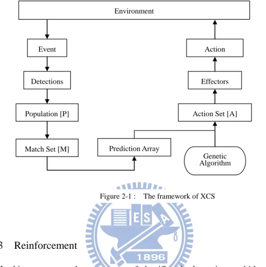
2.1.2 Performance

The performance component presents the overall XCS framework, shown in Figure 2-1. The population of XCS starts with randomly generated classifiers or no classifiers. When an event occurs, XCS forms a match set [M] of classifiers which match the event in the whole population [P]. Then, the system prediction is measured for each action. The system prediction for each action is placed in the prediction array for action selection. If no classifiers match, a covering mechanism is applied to create classifiers that match each of the possible actions and place them in [M]. The system selects an action from the prediction array and forms an action set [A]. Finally, the chosen action is executed, and an environmental payoff may be returned.

(17)

6

2.1.3 Reinforcement

In this component, the parameters of classifiers in the action set [A] to achieve higher accuracy and to complete mappings of the problem space. The procedure for updating the parameters is as following:

 The errors are updated: .  The predictions are updated: .

 The accuracy of a classifier is measured: .

 A relative accuracy of each classifier is determined: .  The Fitness are updated by: .

And the definition of variables is:

 : The fall of rate in the fitness evaluation.

Figure 2-1 : The framework of XCS Environment

Event

Detections

Population [P]

Match Set [M] Prediction Array

Action Set [A] Effectors

Action

Genetic Algorithm

(18)

7

 : Learning rate for updating fitness, prediction, prediction error, and action set size estimate in XCS classifiers.

 : Environment return payoff.  : Prediction error of classifier j.  : Prediction of classifier j.  : Accuracy of classifier j.  : Fitness of classifier j.

Butz [7] indicated that operation will become faster in simple problems if the prediction update comes before the error update, but this may create some problem for complex tasks. Butz and Wilson [8] proposed that it seems to work better to put the error update before the prediction update.

2.1.4 Discovery

The discovery component is exploited to generate new classifiers in the system. XCS executes genetic algorithm (GA) in the current action set [A] when the average time exceeds a threshold . GA usually uses one-point crossover and bitwise mutation on the rule set to generate new rules. Two classifiers are selected with a probability proportional to their fitness values first. After reproducing, crossing, and mutation the parent classifier, two offspring classifiers are generated. And the resulting offspring is inserted into the population [P]. If the size of population [P] is at its maximum value, a proposed method by Kovacs [9] can be adopted to determine the probability of a deletion of a classifier and to remove the low-fitness classifier.

(19)

8

2.1.5 Macroclassifiers

The macroclassifiers are a type of classifiers with the numerosity parameter num in XCS. A macroclassifier is used to speed processing and provide a more perspicuous view of population contents. Whenever XCS generates a new classifier, at the initialization step or at later stages, the population [P] is scanned to examine whether the new classifier has the same condition and action as any existing macroclassifier does. If so, the new classifier is not actually inserted into the population and is therefore deleted, and the numerosity of the existing macroclassifier is incremented by one. Otherwise, the new classifier is added to the population [P] with its own numerosity field set to one. Similarly, when the macroclassifier suffers a deletion, its numerosity is decremented by one, instead of being actually deleted. If the numerosity of a macroclassifier becomes zero, the system removes the macroclassifier from the population.

2.1.6 Covering and Subsumption

Covering and Subsumption are two important components of XCS. Covering is another method to introduce new classifiers into the population. When an environment event occurs and the match set does not contain all possible actions defined for the environment, the covering operation will generate classifiers to match this event for improving the accuracy. The condition of the new classifier created through covering is made to match the current system input, and it is given an action chosen at random. Each attribute in the condition is mutated to don’t care (#) with a probability. Finally, the system puts the newly generated classifier into the population.

In addition to introducing new classifiers into the population, we also have to deal with rules with the same meaning in XCS’s framework. The subsumption

(20)

9

operation is designed to make a rule that absorb other rules if it is more general than other rules and to improve the generalization capability of XCS. There are two forms of subsumption, GA-subsumption and Action-subsumption. In GA-subsumption, when new classifiers are generated, they are examined to see whether their conditions are subsumed by their parent classifiers or not. If the parent classifiers are more general than the new classifiers, the new classifiers are subsumed by the parents. The new classifiers will not be added to the population but numerosity of the parent classifiers is incremented. Otherwise, the system puts the new classifiers into the population. Action-subsumption is different from GA subsumption. Each action set is searched the most general classifier R. Then, all other classifiers in the set are compared to R to see whether R subsumes them. The subsumed classifiers are deleted from the population.

2.1.7 Flow of XCS

At first, XCS initializes the rule set with zero reward randomly. There are four steps for the rule evaluation cycle. The steps are show as following:

1. The state of the environment is detected by detectors.

2. The system examines the condition part of each rule to determine the match set. 3. The match set will be grouped into different sets based on their own actions, and

the prediction payoff for each action is calculated to determinate the action set. 4. Effectors implement the action in the environment, get the reward, and distribute

it to the rules in the action set.

After a specified period of time, GA is executed to generate new rules and delete unfit rules in the rule discovery cycle. Wilson [2] indicated that they can find the classification rules with high accuracy with this framework.

(21)

10

2.2 XCSI

Since in XCS, many problems involve integer attributes, an adaptation of it, the XCSI [11], for the integer domain is adopted. Different from XCS, XCSI is modified in its input interface, mutation, covering and subsumption.

XCSI changes the classifier condition from a string of {0,1,#} to a concatenation of the interval predicates, , where and are integers and denote the lower bound and the upper bound. A classifier matches an input with attributes

if and only if for all .

The mutation operator in XCSI is different from XCS. Wilson indicates that the best method to mutate an allele by adding a value , where is a fixed integer, picks an integer randomly from , and the sign is selected equiprobably.

The covering occurs if there is no classifier matches . In XCSI, the new condition has components , where each and each . The value is a fixed integer and picks an integer randomly from .

An interval predicate subsumes another predicate if and . The subsumption of a classifier by another is defined if every interval predicate in the first classifier’s condition subsumes the predicate in the second classifier’s condition.

2.3 Related Work

Learning Classifier Systems (LCS) are rule-based classifiers that learn the best action of the given inputs. LCS was first described by Holland [1], who proposed a framework that included the condition sensor, reinforcement learning, internal memory, and rule generation by using a genetic algorithm (GA).

(22)

11

To solve the shortcomings of the LCS such as overgeneralization and the difficulty to implement a comprehensive system, Wilson proposed a minimalist version LCS, called Zeroth-Level Classifier System (ZCS) [10] in 1994. ZCS keeps the framework of LCS but simplifies it to increase understandability and performance. But there are still some problems in ZCS, such as path habits and recombination rules from entirely different niches. A path habit is that ZCS may converge onto suboptimal rules and recombining rules from different niches will generate some useless rules.

Recognizing these drawbacks, Wilson proposed XCS, which is currently the most widely used classifier system, and has shown good results on data mining tasks [3, 4]. The accuracy is used by XCS to determine its fitness to avoid the path habit problem and applies recombination to the action set for making meaningful rules. Although XCS has both good performance and knowledge visibility in many problems, the binary inputs of XCS that are unsuitable for many inference problems with integer attribute.

Wilson proposed an adaptation of XCS for integer input called XCSI [11]. XCSI is recently applied to the Wisconsin Breast Cancer (WBC) dataset with the performance results exceeding to other machine learning methods. However, it usually produces a large number of rules which will lower the readability of the classification model. In this study, a new mutation called Bit Mask is devised to reduce the number of classification rules and therefore to improve the readability of the generated prediction model.

(23)

12

Chapter 3 XCS with Bit Mask

3.1 Introduction to Bit Mask

As describe above, XCS is a promising methodology because of its versatility and capability. However, it is known to generate a lot of rules, which lower the readability of the resultant classification model. That is, People may not be able to get the needed knowledge or useful information out of the model.

XCS with bit-mask is proposed to solve such a problem. The adopted bit-mask is used to detect the stable building blocks in classifiers and to prevent crossover and mutation operators from unnecessarily altering them. Consequently, the resultant classification model needs fewer rules than that evolved by the original XCS to achieve the same level of accuracy.

In this chapter, we will first present the concept and mechanism of bit-mask into XCS. Then, we discuss where bit-mask can be implemented. And we channel how bit-mask applied to different environments.

3.2 Representation

In order to apply Bit Mask to XCS classifiers, the representation of XCS rules is modified to make them capable of finding a set of stable building blocks and unnecessarily altering attributes. For this purpose, a parameter called bit mask (BM) is added into the classifier representation as:

< Classifier >::= < Condition >:< Action >:< BM >: < Payoff prediction >:< Payoff error >: < Fitness >

(24)

13

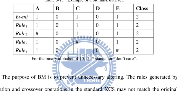
crossover operators. Rules with BM will be more stable than the standard XCS rules and will result in fewer classifiers when the mutation and crossover operation is triggered. For example, if the rules of the condition and the action are set as Table 1, the attribute B and D are determined as stable building blocks in BM. Different from the standard XCS, when the mutation and crossover operation occur, the condition attributes in BM will not be altered to avoid generating redundant rules.

Table 3-1: Example of a bit mask data set.

A B C D E Class Event 1 0 1 0 1 2 Rule1 1 0 1 0 1 2 Rule2 # 0 1 0 1 2 Rule3 1 0 # 0 1 2 Rule4 1 0 1 0 # 2

For the binary alphabet of {0,1}, # stands for “don’t care”.

The purpose of BM is to prevent unnecessary altering. The rules generated by mutation and crossover operations in the standard XCS may not match the original event and some redundant rules might occur. Through the bit mask mechanism, the rule with BM can prevent altering stable building blocks. The collection of rules will strongly support the original event, and may cover more subset of cases.

3.3 Algorithm of XCS with Bit Mask

In XCS, each rule contains one condition and one action, and the condition contains n attributes. Because of the relation between conditions and actions, the attributes also have influence on the actions. That is, when one attribute is changed, it may produce a different action. The connection between attributes and actions is the main idea of bit-mask. Given an environmental state, a match set will be formed in

(25)

14

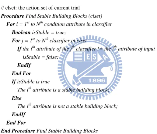
the usual way [10], and its action is chosen by the system. Once an action is chosen, the system forms an action set which consists of the classifiers in match sets advocating the chosen action. If the chosen action is the same as the environmental action, each attribute of the classifiers in action set will be scanned. If all the nth attribute of classifiers in action set is same as the nth attribute of the environmental input, the nth attribute will be set as a stable building block. The definition of variables and the pseudo code for Find Stable Building Blocks are shown in Figure 3-1.

// clset: the action set of current trial

Procedure Find Stable Building Blocks (clset)

For i = 1st to Nth condition attribute in classifier Boolean isStable = true;

For j = 1st to Nth classifier in clset

If the ith attribute of the jth classifier != the ith attribute of input isStable = false;

EndIf

End For

If isStable is true

The ith attribute is a stable building block; Else

The ith attribute is not a stable building block; EndIf

End For

End Procedure Find Stable Building Blocks

The set of stable building blocks called bit mask (BM). The current BM will be set if the classifier has no BM. However, the current BM can’t be set directly if a BM already exists in the classifier. The current BM has to be compared with the BM of the classifier. If the current nth building block is also in the stable building block set of the classifier, the nth building block will be remained. Otherwise, the nth building

(26)

15

block will be removed, and the new BM will be set on the classifier. The definition of variables and the pseudo code for Set Stable Building Blocks are shown in Figure 3-2.

// cl: classifier

// BM: the BM find in action set of current trial // cl.BM: the BM of the classifier

//NewBM: the new BM generate from BM and cl.BM

Procedure Set Bit Mask( cl, BM)

Boolean[] NewBM; If the classifier is no BM cl. BM = BM; Else

For i = 1st to Nth condition attributes if cl.BM(i) is true and BM(i) is true

NewBM(i) is true; Else NewBM(i) is false End if End For cl.BM = NewBM; End If

End Procedure Set Bit Mask

After setting BM in classifiers, we changes crossover and mutation operations in the GA mechanism. In mutation mechanism, the condition attributes in BM are stable, and will not be mutated. But the other attributes will be altered same as the standard XCS. In crossover mechanism, if the two condition attributes are both in BMs, the attributes will not perform crossover. But the other attributes will perform crossover, and the new classifier will insert into population. If the size of classifiers is larger than the size of environment, the compensating deletion occurs as the standard XCS.

(27)

16

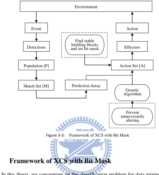
3.4 Framework of XCS with Bit Mask

In this thesis, we concentrate on the classification problem for data mining. We model the relation between attribute and class in a rule. With this interpretation, we make XCS a classification system. The overall framework of XCS with bit-mask is shown in Figure 3-3. Different from the original XCS framework, XCS with bit-mask can be applied to much type of problems. It focuses on the bit mask mechanism and problem of classification.

With the bit-mask capable representation and the corresponding operations, we now describe the flow of XCS with bit-mask. We first consider the data set of a classification problem as an environment. To simulate the occurrence of events, data items of the data set to classify are selected randomly or sequentially as the system input. The number of covering actions in match set is formed by the original XCS.

Figure 3-3: Framework of XCS with Bit Mask Environment

Event

Detections

Population [P]

Match Set [M] Prediction Array

Action Set [A] Effectors Action Genetic Algorithm Find stable building blocks and set bit mask

Prevent unnecessarily

(28)

17

Thus, the action set can be formed. The Bit Mask mechanism is applied on the action set to detect the stable building blocks and record stable building blocks on the classifier. When the genetic algorithm is triggered, it will prevent unnecessarily altering in mutation and crossover operators. Compare to the operations conducted in the standard XCS, the bit-mask mechanism may let generate fewer redundant rules.

(29)

18

Chapter 4 Experimental Results

In previous chapters, we have briefly reviewed the original XCS framework, introduced the concept of bit-mask, and described the purpose of XCS with bit-mask in detail. In this chapter, we employ the XCS and XCS with bit-mask to deal with some experiments and compare the performances, system errors, and population sizes. The performance refers to the fraction of the last 50 exploit trials that were correct. The system error refers to the absolute difference between the system prediction for the chosen action and the actual external payoff, divided by the total payoff range (1000) and the average over the last 50 exploit trials. The population size refers to the number of macroclassifiers. We use the XCS system publicly on the Internet [12]. And the XCS system is modified to include the mechanisms described in chapter 3 to establish the XCS with bit-mask system for testing. Each experiment is conducted for 200 independent runs, and the statistics averaged over the 200 runs are reported.

4.1 Experimental Data Sets

To briefly see the behavior of XCS with bit-mask behavior, we divide experiments to three parts to improve the bit-mask mechanism.

 Boolean Multiplexer

First, we employ both XCS and XCS with bit-mask to tackle the boolean multiplexer function of three different sizes, including 6 bits, 11 bits and 20 bits. Boolean multiplexer functions are defined for binary strings of length . The function result is determined by treating the first k bits as an address that indexes into the remaining 2k bits, and the value of the indexed bit, either 0 or 1, is the function result.

(30)

19

 Integer Test Function

Second, we employ them to deal with integer datasets. The integer datasets are some synthetic oblique data sets [11]. The first dataset, “Random-Data2”, was constructed by random vectors (x1 , x2), with each xi a random integer from (1 , 10).

The current outcome o for each vector was selected according to

(1) An instance of Random-Data2 is composed by a vector and its outcome. The second random dataset, “Random-Data9”, was constructed like Random-Data2 as follows. Radom-Data9 has nine dimensions and the expression determining the outcome was (2)

 Real World Data - Wisconsin Breast Cancer

We use them to deal with the real world data, Wisconsin Breast Cancer (WBC) Database which was donated to the UCI Repository [13] by Prof. Olvi Mangasarian and contains 699 instances collected over time by Dr. William H. Wolberg. Each instance of WBC database has nine attributes which are Clump Thickness, Uniformity of Cell Size, Uniformity of Cell Shape, Marginal Adhesion, Single Epithelial Cell Size, Bare Nuclei, Bland Chromatin, Normal Nucleoli, and Mitoses. Each attribute has a value between 1 and 10 inclusive. Small sample of raw data is shown as follow:

1000025,5,1,1,1,2,1,3,1,1,2 1002945,5,4,4,5,7,10,3,2,1,2 1015425,3,1,1,1,2,2,3,1,1,2 1016277,6,8,8,1,3,4,3,7,1,2 1017023,4,1,1,3,2,1,3,1,1,2

The first number is a label, the next nine attributes are the attributes, and the last is the class level, 2 for Benign and 4 for Malignant.

The three parts of experiment described before show how XCS and XCS with 1017122,8,10,10,8,7,10,9,7,1,4

1018099,1,1,1,1,2,10,3,1,1,2 1018561,2,1,2,1,2,1,3,1,1,2 1033078,2,1,1,1,2,1,1,1,5,2 1033078,4,2,1,1,2,1,2,1,1,2

(31)

20

bit-mask classify datasets in data mining. From the classifying of the simple data set, and boolean multiplexer function, it is shown that the XCS with bit-mask is as feasible as the standard XCS. But the result of this experiment doesn’t directly indicate that bit-mask mechanism is workable. We applied bit-mask mechanism to integer domain and compared with the standard XCS. At last, the real world data set can be viewed as a benchmark to display that the bit-mask mechanism can not only classify dataset but also decrease the redundant rules. The experimental results are presented in the follow sections.

4.2 Result in Boolean Multiplexer

4.2.1 6-bit Multiplexer

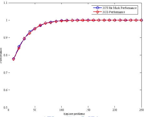
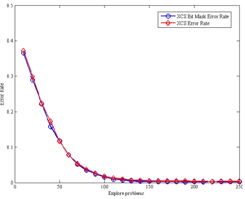
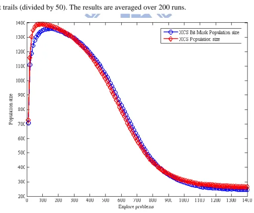
Figure 4-1, 4-2, 4-3 show the experimental results for the boolean multiplexer of 6-bits. Figure 4-1 shows the performance between XCS and XCS with bit-mask, Figure 4-2 shows the population size, and Figure 4-3 shows the system error rate. As we can observe, XCS gets approximately 100 % performance in 4000 exploit trails, and XCS with bit-mask gets approximately 100% performance in 4000 exploit trails, too. For the system error, XCS gets approximately 0% system error in 6000 exploit trails, and XCS with bit-mask gets approximately 0% system error in 6000 exploit trails. Finally, XCS evolves the population with 29.47 classifiers, and XCS with bit-mask evolves the population with 25.01 classifiers. Parameters of the experiment are , , , , , , , , and .

Base on the experimental results, we can find that XCS and XCS with bit-mask can achieve the same performance, system error rate, and population size when the exploit trails is appropriate. Thus, it can be shown that XCS and XCS with bit-mask have the same speed of convergence. However, the effect of applying bit mask into

(32)

21

XCS appears. XCS with bit-mask can save 15.13% of population size for 6-bit multiplexer over the 200 runs on average.

Figure 4-2: Population size of experimental results for 6-bit multiplexer

Population size is the number of macroclassifiers. Explore problems is in exploit trails (divided by 50). The results are averaged over 200 runs.

Figure 4-1: Performance of experimental results for 6-bit multiplexer

Performance is the fraction of the last 50 exploit trials that were correct. Explore problems is in exploit trails (divided by 50). The results are averaged over 200 runs.

(33)

22

4.2.2 11-bit Multiplexer

Figure 4-4 ~ 4-6 show the experimental results for the 11-bits boolean multiplexer. Figure 4-4 shows the performance between XCS and XCS with bit-mask, Figure 4-5 shows the population size, and Figure 4-6 shows the system error rate. From the figures, the performance of XCS reached approximately 100 % in 8000 exploit trails, and the performance of XCS with bit-mask reached approximately 100% in 8000 exploit trails, too. For the system error, the system error of XCS gets approximately 0% in 12000 exploit trails, and the system error of XCS with bit-mask gets approximately 0% in 12000 exploit trails. For the population size, the population size of XCS is evolved with 81.51 classifiers, and the population size of XCS with bit-mask is evolved with 74.85 classifiers. The experimental parameters are , , , , , , , , and .

From the experimental results, we can acquire that the 11-bit multiplexer has

Figure 4-3: Error rate of experimental results for 6-bit multiplexer

Error rate is the fraction of total payoff range. Explore problems is in exploit trails (divided by 50). The results are averaged over 200 runs.

(34)

23

similar outcome to 6-bit multiplexer. In this experiment, XCS with bit-mask on average saves 8.1% of population size over 200 runs.

(35)

24

4.2.3 20-bit Multiplexer

Figure 4-7 ~ 4-9 demonstrate the experimental results for the boolean multiplexer of 20-bits. Figure 4-7 shows the performance between XCS and XCS with bit-mask, Figure 4-8 shows the population size, and Figure 4-9 shows the system error rate. From the result, XCS gets approximately 100 % performance in 35000 exploit trails, and XCS with bit-mask gets approximately 100% performance in 35000 exploit trails, too. For the system error, XCS gets approximately 0% system error in 50000 exploit trails, and XCS with bit-mask gets approximately 0% system error in 50000 exploit trails. For the population size, XCS evolves the population with 261.52 classifiers, and XCS with bit-mask evolves the population with 247.67 classifiers. For 20-bit multiplexer, XCS with bit-mask saves 5.2% of the population size. The experiment Parameters are as follow : , , , ,

, , , , and .

Error rate is the fraction of total payoff range. Explore problems is in exploit trails (divided by 50). The results are averaged over 200 runs.

(36)

25

(37)

26

4.3 Result in Integer Test Function

4.3.1 2 dimensions

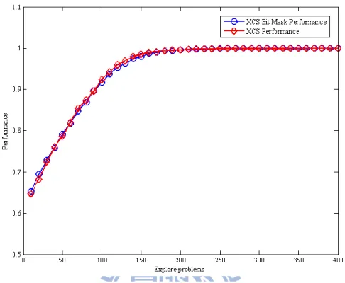
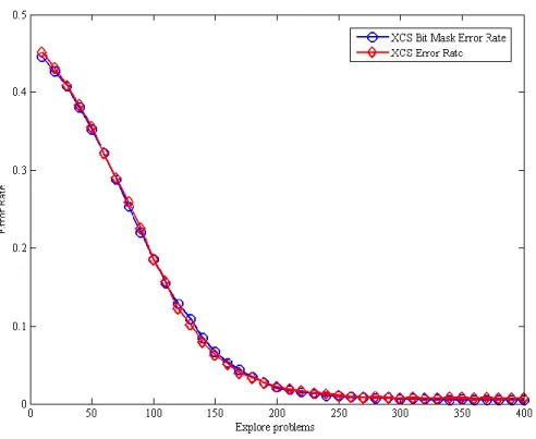
Figure 4-10, 4-11, and 4-12 show the experimental results for the two dimensions of integer, Random-Data2. For the performance at figure 4-10, XCS gets approximately 95 % performance in 20000 exploit trails, and XCS with bit-mask gets approximately 95% performance in 20000 exploit trails, too. For the system error at figure 4-11, XCS gets approximately 10% system error in 15000 exploit trails, and XCS with bit-mask gets approximately 10% system error in 15000 exploit trails. For the population size at figure 4-12, XCS evolves the population with 51.3 classifiers, and XCS with bit-mask evolves the population with 32.73 classifiers.Parameters of the experiment are , , , , , , , , and .

Base on the experimental results in integer, we can find that XCS and XCS with

Error rate is the fraction of total payoff range.. Explore problems is in exploit trails (divided by 50). The results are averaged over 200 runs.

(38)

27

bit-mask obtain the same performance and system error rate in the synthetic oblique data. But for the population size, the effect of bit mask is significant in integer. As we can see, XCS with bit-mask on average saves 36.21% of population size over 200 runs.

Figure 4-10: Performance of experimental results for 2 dimensions

(39)

28

Figure 4-12: Error rate size of experimental results for 2 dimensions

Figure 4-11: Population size of experimental results for 2 dimensions

(40)

29

4.3.2 9 dimensions

Figure 4-13, 4-14, 4-15 demonstrate the experimental results for the nine dimensions of integer, Random-Data9. First, Figure 4-10 shows the performance between XCS and XCS with bit-mask. XCS gets approximately 90 % performance in 28000 exploit trails, and XCS with bit-mask gets approximately 90% performance in 28000 exploit trails, too. Second, Figure 4-11 shows the population size. XCS evolves the population with 542.38 classifiers, and XCS with bit-mask evolves the population with 356.23 classifiers. Finally, Figure 4-12 shows the system error rate. XCS gets approximately 20% system error in 25000 exploit trails, and XCS with bit-mask gets approximately 20% system error in 25000 exploit trails. Parameters are , , , , , , , , and . In this experiment, the result is similar to Random-Data2. XCS with bit-mask on average saves 34.32% of the population size over 200 runs.

Figure 4-13: Performance of experimental results for 9 dimensions

(41)

30

Figure 4-15: Error rate of experimental results for 9 dimensions

Figure 4-14: Population size of experimental results for 9 dimensions

(42)

31

4.4 Results in Wisconsin Breast Cancer

In this section, we applied XCS and XCS with bit-mask to the WBC dataset in the stratified tenfold cross-valuation procedure in which the system learned on the part of the data and were test on the reminder. “Tenfold cross-valuation” is a standard way of measuring the error rate of learning scheme on particular dataset [14]. Described the procedure briefly, the dataset is divided into 10 parts called “fold”. The system is tested on each fold after being trained by the other 9 folds. Then the results of the 10 test fold are average to a final score.

Figure 4-16 ~ 4-18 show the results of the performance, the population size, and the system error rate for WBC dataset. The performance of XCS reaches approximately 95% in 5000 exploit trails, and the performance of XCS with bit-mask gets approximately 94% in 9000 exploit trails. For system error rate, XCS gets approximately 6% system error in 4000 exploit trails, and XCS with bit-mask gets approximately 7% system error in 9000 exploit trails. For the population size, XCS evolves the population with 271.23 classifiers, and XCS with bit-mask evolves the population with 94.58 classifiers.

XCS XCS with bit-mask #1 0.942 0.9 #2 0.942 0.914 #3 0.971 0.942 #4 0.914 0.928 #5 0.9 0.957 #6 0.957 0.914 #7 0.957 0.9 #8 0.9 0.914 #9 0.928 0.957 #10 0.914 0.928 Avg. 0.9325 0.9254

(43)

32

The ten test results of XCS and XCS with bit-mask are shown in Table 4-1. It can be seen that XCS gets 93.25% of correct rate, and XCS with bit-mask also obtains 92.54% of correct rate. In this experiment, the performance of bit-mask is similar to the original XCS. But the population size of bit-mask is smaller than the original XCS in WBC dataset.

Figure 4-16: Performance of experimental results for WBC

Performance is the fraction of the last 50 exploit trials that were correct. Explore problems is in exploit trails (divided by 100). Parameters are , , , , , ,

(44)

33

Figure 4-17: Population size of experimental results for WBC

Population size is the number of macroclassifiers. Explore problems is in exploit trails (divided by 100). Parameters are , , , , , , , , and

.

Figure 4-18: Error rate of experimental results for WBC

Error rate is the fraction of total payoff range.. Explore problems is in exploit trails (divided by 100). Parameters are , , , , , , , , and

(45)

34

4.5 Discussion

Base on the experiments of the previous sections, we discovered two interesting points. First, the bit-mask mechanism can save the population size more in integer domain than in boolean domain. Second, it saves more rules in WBC dataset than in synthetic oblique dataset. As for 6-bit, 11-bit, and 20-bit multiplexer, the bit-mask only saves less than 20% of the population size. But in integer domain, it saves 30-40% of the population size. The difference between boolean and integer is significant. When XCS is applied in boolean multiplexer, the rule’s representation is {0,1,#}, it’s easy to define whether the rule is accepted or not. But in Integer domain, the rule’s representation is , where and are integers and denote the lower bound and the upper bound. A rule matches an input with attributes if and only if for all . There is some elasticity in integer. According to the conception, when using the bit-mask mechanism to avoid altering crossover and mutation operators, it will not produce redundant rules. The population size of system will be saved.

The bit-mask mechanism saves 65% rules in WBC dataset, but only saves 30-40% rules in synthetic oblique dataset. The class of the synthetic oblique dataset, Random-Data2 and Random-Data9, is made by the sum of the attributes. If the sum of attributes in bigger than the assigned number, the class will set to 1. Otherwise, the class will set to 0. The outcome defined by this doesn’t model the relation between attribute and class. There is not any directly connection between attribute and class. Unlike the real world dataset, WBC, each of attributes may give a huge influence of the class level. Therefore, the bit-mask mechanism works better in WBC dataset than in synthetic oblique dataset.

(46)

35

Chapter 5 Conclusions

5.1 Summary

In this paper, we first reviewed XCS briefly, followed by the introduction of the concept of bit mask. After applying bit mask to XCS, we described the purpose of the mechanism bit-mask and show the framework of it in detail. Finally, we implemented XCS with bit-mask by modifying the existing XCS system and did a series of boolean multiplexers, integer dataset, and real world dataset for both XCS and XCS with bit-mask. By comparing the experimental results, two interesting points are discussed. Bit mask performed better in integer domain than in boolean domain. Because of the concept of bit mask is the relation between attribute and class, bit mask modeled the real world data better than the synthetic oblique datasets. The experimental results confirmed that bit mask can detect the stable building blocks, avoid unnecessary altering and save the redundant rules in data mining.

5.2 Contributions

By the experimental results show in this paper, with the bit mask mechanism, it can be applied to data mining and make the least rules to explain the dataset. The contributions of bit mask are as follow:

 XCS generate redundant rules in mutation and crossover operator in GA.  XCS works poorer in integer domain than in boolean domain.

 According to the experiments, bit mask can saves the rules in XCS.

 Applying bit-mask mechanism performs better in integer domain than in boolean domain.

 Using bit mask can help XCS to promote performance

(47)

36

By bit mask mechanism, people can get the required information or knowledge from the evolved classification model. The real world dataset can be detected more interesting information and help people to understand the implication of data with it. Therefore, it may be proven a useful technique for data mining application.

5.3 Future Work

Further work is needed, in a variety of environments, to increase understanding of the technique. In particular, the bit mask not did well in simple dataset such as boolean multiplexers, there may be other methods to limit the number of bit mask that make it better. Besides boolean and integer dataset, real number dataset should be looked at. As for bit mask itself, interesting research topics and directions, including theoretical understanding and algorithmic improvement, are waiting to be explored. Research along this line should be continuously pursued and conducted in order to develop classification systems that are not only feasible in theory but also viable in practice to further advance all the related domains and disciplines.

(48)

37

REFERENCE

[1] Holland, J. H. (1975). Adaptation in natural and artificial systems. University of Michigan Press. ISBN: 0-2625-8111-6.

[2] Wilson, S. W. (1998). Generalization in the XCS classifier system. In

Proceedings of the Third Annual Conference on Genetic Programming (GP 98),

pages 665–674.

[3] Stone, C. and Bull, L. (2003). For real! XCS with continuous-valued inputs.

Evolutionary Computation, 11(3):299–336.

[4] Wilson, S. W. (2000b). Mining oblique data with XCS. Lecture Notes in

Computer Science, 1996:158–176.

[5] Pei, J., Tung, A. K. H., and Han, J., Fault-tolerant frequent pattern mining: Problems and challenges. In Proceedings of 2001 ACM SIGMOD Workshop on

Research Issues in Data Mining and Knowledge Discovery (DMKD), 2001.

[6] Han, J. and Kamber, M. (2005). Data Mining: Concepts and Techniques. Morgan Kaufmann. ISBN: 1558609016.

[7] Butz, M. V., Kovacs, T., Lanzi, P. L., and Wilson, S. W. (2001). How XCS evolves accurate classifiers. In Proceedings of the Genetic and Evolutionary

Computation Conference, pages 927–934.

(49)

38

Lecture Notes in Computer Science, 1996:253–272.

[9] Kovacs, T. (1999). Deletion schemes for classifier systems. In Proceedings of

the Genetic and Evolutionary Computation Conference 1999 (GECCO-99),

pages 329–336.

[10] Wilson, S. W. (1994). ZCS: A zeroth level classifier system. Evolutionary

Computation, 2(1):1–18.

[11] Wilson, S. W. (2000b). Mining oblique data with XCS. Lecture Notes in

Computer Science, 1996:158-176.

[12] Butz, M. V. (2000). Java implementation of XCS.

ftp://ftp-illigal.ge.uiuc.edu/pub/src/XCSJava/XCSJava1.0.tar.Z.

[13] Blake, C. and Merz, C. (1998) UCI repository of machine learning databases. http://www.ics.uci.edu/mlearn/MLRepository.html.

[14] Witten. I. H. and E. Frank. (2000). Data Mining: Practical Machine Learning

Tools and Techniques with Java Implementations. San Francisco, CA: Morgan

在 XCS 分類系統中導入位元遮蔽機制以進行資料探勘

國

立

交

通

大

學

資訊科學與工程研究所

碩

士

論

文

在 X C S 分 類 系 統 中 導 入 位 元 遮 蔽 機 制

以進行資料探勘

XCS with Bit Mask in Data Mining

研 究 生：林佳慧

指導教授：陳穎平 教授

在 XCS 分類系統中導入位元遮蔽機制以進行資料探勘

XCS with Bit Mask in Data Mining

研 究 生：林佳慧 Student：Jia-Huei Lin

指導教授：陳穎平 Advisor：Yi-Ping Chen

國 立 交 通 大 學

資 訊 科 學 與 工 程 研 究 所

碩 士 論 文

在 XCS 分類系統中導入位元遮蔽機制以進行資料探勘

學生：林佳慧 指導教授：陳穎平

國立交通大學資訊科學與工程研究所

摘 要

在本篇論文中提出了一種改進 XCS 以達到減少規則(Classifier)

數量的方式。XCS 是學習型分類系統(Learning Classifier System)中的

一個分支，已經被證明能夠提供精確而又最具一般性規則集合的分類

系統。但是，它通常會產生過多的規則，而降低分類模型的可讀性。

也就是說，人們可能無法自模型中獲得所需的知識或有用的信息。為

了解決這個問題，提出一個位元遮蔽機制加入 XCS 系統(XCS with Bit

Mask)，以達到減少規則數量的目的，從而提高生成的分類模型的可

讀性。

我們做了一系列來研究該方法，針對布爾(Boolean) 輸入，利用

N 位元的多工器(N-bit multiplexer)進行實驗，包括 6 位元、11 位元和

20 位元。對於整數輸入，利用兩個人造的資料集合 ─ Random Data2

和 Random Data2 來比較 XCS 和加入此方法的 XCS 系統。此外，也

引入現實世界的數據進行實驗。根據實驗結果，驗證該方法可以達到

減少規則數量並提升精度高的目的。

關鍵字：XCS 分類系統、學習型分類系統、群體數量、位元遮蔽機

制、資料探勘

ABSTRACT

誌 謝

感謝這兩年來辛苦教導的陳穎平教授，平時安排個人研究會議進

行指導與教誨，於研究期間發生任何問題，教授都會在一旁提點該注

意的事情，不僅是求學研究上的知識，也包括了做人做事的道理。當

我碰到困難時，會在第一時間幫助我解決問題，致上由衷的感謝。

謝謝口詴委員楊進木教授、陳宜欣教授及陳穎平教授針對論文上

的錯誤給予建議，使得論文整體更加詳細清楚，誠摯感謝。

最重要的感謝，莫過於我的父母及家人，不管是給予我物質上的

幫助亦或是提醒我生活上該注意的大小事務，沒有你們的支持及鼓勵，

憑著自己一人的努力是無法成就現在的我。

種種的支持及鼓勵，讓我點滴在心頭，雖然是短短幾行敘述，但

代表了我無限的感恩，謝謝你們!

CONTENTS

LIST OF FIGURES

LIST OF TABLES

Chapter 1

Introduction

1.1 Motivation

1.2 Research Objective

1.3 Organization of the Thesis

Chapter 2

A Brief Review of XCS

2.1 XCS

2.1.1 Representation

2.1.2 Performance

2.1.3 Reinforcement

2.1.4 Discovery

2.1.5 Macroclassifiers

2.1.6 Covering and Subsumption

2.1.7 Flow of XCS

2.2 XCSI

2.3 Related Work

Chapter 3

XCS with Bit Mask

3.1 Introduction to Bit Mask

在 X C S 分類系統中導入位元遮蔽機制

研究生：林佳慧

指導教授：陳穎平教授

研究生：林佳慧 Student：Jia-Huei Lin

國立交通大學

資訊科學與工程研究所

碩士論文

學生：林佳慧指導教授：陳穎平

摘要

誌謝