基於拉格朗日最佳化針對 H.264 畫面內編碼的位元率控制演算法

(1)

國立交通大學

資訊科學與工程研究所

碩士論文

基於拉格朗日最佳化

針對 H.264 畫面內編碼的位元率控制演算法

Lagrangian-Optimization based Intra Frame Rate Control

for H.264/AVC

研究生：周鼎力

指導教授：蔡文錦博士

(2)

基於拉格朗日最佳化針對 H.264 畫面內編碼的位元率控制演算法

Lagrangian-Optimization based Intra Frame Rate Control for H.264/AVC

研究生：周鼎力 Student：Ting-Li Chou

指導教授：蔡文錦 Advisor：Wen-Jiin Tsai

國立交通大學

資訊科學與工程研究所

碩士論文

A Thesis

Submitted to Institute of Computer Science and Engineering College of Computer Science

National Chiao Tung University in partial Fulfillment of the Requirements

for the Degree of Master

in

Computer Science

June 2009

Hsinchu, Taiwan, Republic of China

(3)

中文摘要

為了讓視訊編碼後的位元率能維持在頻寬的限制之內，並且達到良好與穩定的畫面品質，位元率控制是相當重要的。然而目前大多數的研究都集中在畫面間編碼(inter frames)而不是容易造成緩衝區溢位的畫面內編碼(intra frames)。此外 Intra-only 這種編碼方式也已經納入 H.264 新的 profile 當中，它較傳統 GOP 編碼更適合應用在特別要求畫面品質的產品上。在此論文中，我們提出一個於 Intra-only 編碼與 GOP 編碼皆適用的位元率控制演算法。首先我們提出基於 Lagrangian 最佳化的 QP 決定方式，藉由位元率與 PSNR 預測模型，我們利用 Lagrangian 最佳化來找出可以平衡畫面品質與編碼效能的 QP 最佳解。另外，為了解決場景變換對位元率控制所產生的影響，在找出場景變換的畫面後，針對其使用以梯度複雜度為基礎的位元率模型來決定適合的 QP，避免緩衝區溢位。實驗結果顯示，提出的方法可以達到更好更穩定的畫面品質，且緩衝內含量也都維持在較低的水平。關鍵字：位元率控制、H.264、畫面內編碼、拉格朗日最佳化、預測模型

(4)

ABSTRACT

Rate control serves as an important technique to constrain the bit rate of video transmission over a limited bandwidth and to control the bit allocations within a video sequence to maximize its overall visual quality. However, most of rate control researches focus on inter coding frames instead of intra coding frames which are more possible to cause buffer overflow problem. Besides, H.264 Intra-only compression scheme has been standardized as H.264 profiles which are more proper for professional applications than

traditional GOP compression scheme.

In this thesis, we propose an improved rate control scheme which is appropriate not only for GOP compression but also for Intra-only compression. First, we present a Lagrangian-optimization based QP determination scheme for I-frames. By the estimation models for rate and PSNR of I-frames, the best quantization parameters can be determined by Lagrangian optimization method. In order to deal with the specific intra frames caused by scene transitions, a gradient complexity based QP determination method is proposed. After detecting scene change frames, the proposed gradient complexity based rate-QS model is adopted to determine appropriate QPs for avoiding buffer overflow and saving bit budget. Simulation results show, that compared to other reference algorithms, our approach achieves better and stable quality with low buffer fullness.

Index Terms: Rate control, H.264, intra frames, Lagrangian optimization, Prediction

(5)

誌謝

本論文是我人生的一大步，願為人類科技的一小步。在這兩年的研究所生涯裡，首先要感謝的是我的指導教授蔡文錦博士，其不辭辛勞的教導使我獲益匪淺，在課業研究上，給予我建議；在人生旅途上，指引我方向，在此謹向我的指導教授蔡文錦博士致上最高的敬意，感謝老師這兩年來對我的用心指導。我要感謝實驗室裡的學長姐蕭家偉、陳信良、李威邦、黃重輔、吳秉承和陳佩詩，在我的研究過程中給予我指導和寶貴的意見。還要感謝我的同學黃子娟、陳建裕、林宜政、林詩凱和吳漢倫，謝謝你們兩年來不管是在課業上的討論、生活上的分享或戰場上的廝殺(笑)，都使我獲益良多。還有謝謝學弟王世明、許智為、潘益群和游顥榆，接下來要靠自己了，願你們明年都能順利畢業。感謝我的父母和弟弟對我的支持，讓我能夠完成大學與研究所學業，步入下一個人生階段。最後感謝我的女朋友奕萱，謝謝你對我的陪伴與鼓勵，能彼此分享生活中的一切，是最棒的一件事。接下來，我將邁入人生的另一個里程，相信有你們的陪伴，未來的路會更寬廣、更美好。謹以此論文獻給我的師長、父母和所有關心我的人

(6)

LIST OF FIGURES

Fig. 1-1 Video transmission system ... 2

Fig. 1-2 (a) Variable bit rate vs. (b) Constant bit rate ... 3

Fig. 1-3 Basic rate control flow ... 3

Fig. 1-4 The chicken egg dilemma for H.264 rate control ... 4

Fig. 1-5 4x4 block intra prediction mode direction[9] ... 6

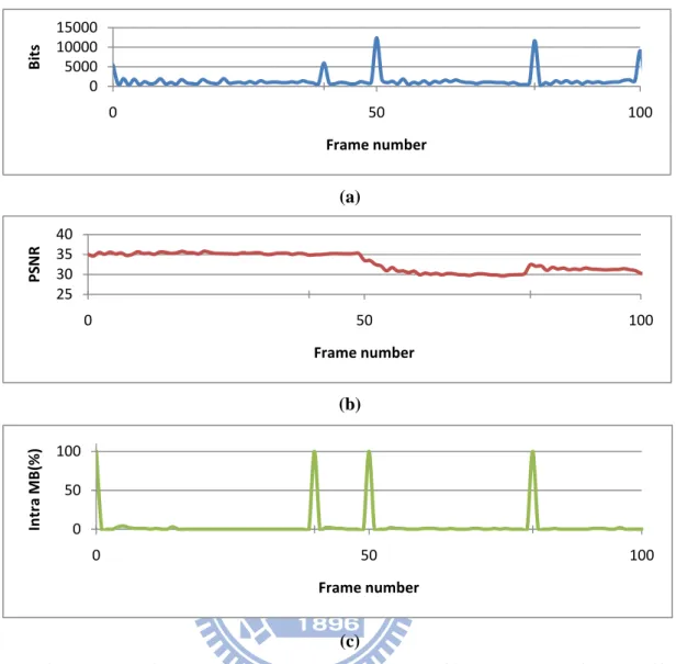
Fig. 1-6 (a) Bits, (b) PSNR and (c) the percentage of intra coded MB for the qcif sequence Akiyo-Foreman which cascaded at 50th frame, and the GOP size is 40 ... 8

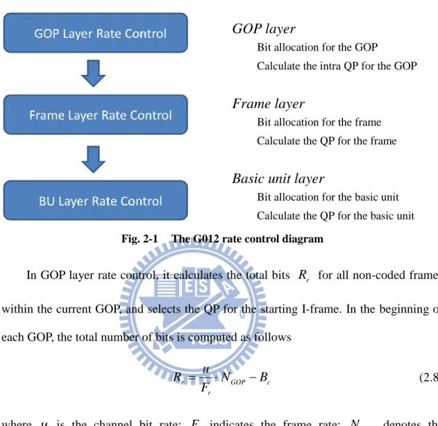
Fig. 2-1 The G012 rate control diagram ... 13

Fig. 2-2 Comparison of Laplacian model vs. Cauchy model[16] ... 16

Fig. 2-3 Intra coded bits vs. gradient per pixel (a) Foreman, QP=36 (b) Carphone, QP=25 ... 17

Fig. 2-4 Curve fitting results of QS versus MSE for different sequences[19] ... 20

Fig. 2-5 The relation between SCI and general I-frames ... 21

Fig. 2-6 The value of parameter a from akiyo sequence ... 22

Fig. 3-1 The curves between Rnorm and QS of Foreman ... 24

Fig. 3-2 The curves between Rnorm and QS of Akiyo ... 25

Fig. 3-3 Prediction error comparison of proposed model and Jing’s model. Analysis from (a) Foreman@QCIF-512kbps and (b) Mobile@QCIF-512kbps ... 27

Fig. 3-4 The relation curves between PSNR and QP of several sequences ... 28

Fig. 3-5 The relation between model parameter, m and frame complexity, G ... 28

Fig. 3-6 The prediction accuracy of Foreman at 512kbps (up), 1024kbps (down) ... 29

Fig. 3-7 Diagram of the proposed non SCI QP determination algorithm ... 32

Fig. 3-8 MDOG value of the QCIF sequence Trevor-Stefan-Silent-Coastguard ... 33

Fig. 3-9 FDs of eight QCIF cascaded sequences when the threshold is set to 35 ... 34

Fig. 3-10 The relation curve between G and G*a ... 35

Fig. 3-11 Prediction error comparison from a cascaded scene change sequence. ... 36

Fig. 3-12 Flow charts for Intra-only compression ... 37

Fig. 4-1 Relation curves between the best initial QP and bpp for News, Foreman, and Mobile[21] ... 40

Fig. 4-2 Flow charts for GOP compression ... 41

(9)

Fig. 5-2 Buffer fullness v.s. frames for Foreman@1024 kbps ... 46 Fig. 5-3 Buffer fullness v.s. frames for Combo2@768kbps ... 47 Fig. 5-4 (a) PSNR v.s. frames (b) Buffer fullness v.s. frames for Mobile@96kbps .. 49

(10)

LIST OF TABLES

Table 1-1 Comparison between Intra-only and GOP compression[10] ... 7 Table 3-1 Detection correctness of two advertisements ... 35 Table 5-1 Performance comparisons for Intra-only scheme ... 44 Table 5-2 Result comparisons of normal sequences for GOP compression scheme .... 48 Table 5-3 Result comparisons of scene change sequences for GOP compression scheme ... 48

(11)

Chapter 1 Introduction and Motivation

For the coming of digital multimedia communication, the demand for the storage and transmission of visual information has stimulated the development of video coding standards, including MPEG-1[1], MPEG-2[2], MPEG-4[3], H.261[4], H.263[5], and H.264/AVC[6].

H.264 is an up-to-date coding standard approved by ITU-T as MPEG 4 - Part 10 Advanced Video Coding (AVC). It includes the latest advances of video coding techniques. H.264 is designed in two layers: a video coding layer (VCL), and a network adaptation layer (NAL). Although H.264/AVC basically follows the framework of prior video coding standards such as MPEG-2, H.263, and MPEG-4, it contains new features that enable it to achieve a significant improvement in compression efficiency.

1.1 Introduction to Rate Control

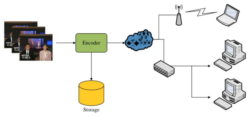
A rate control algorithm which meets a constrained channel rate by controlling the number of generated bits is necessary to encoder. Either the coded video is transmitted over the Internet or stored in a storage device, there is a bandwidth constraint to limit the bit rate of videos. Although the transmission bandwidth is growing larger over the years, more exquisite videos with high resolutions, such as HD and Full HD, are becoming popular. These high definition videos consume much more bit rate than the traditional definition videos. Encoding video without rate control will suffer from

(12)

happen. Fig. 1-1 shows the two mentioned examples. Hence, rate control is a key issue of the modern video coding researches.

The generated bits and video quality of an encoder highly rely on several coding parameters, especially the quantization parameter (QP). In particular, choosing a large QP reduces the resulting bit rate and meanwhile the visual quality of the encoded video is reduced. For illustration, Fig. 1-2(a) shows that if the QP is constant, the resulting video is at a stable quality with a variable bit rate (VBR). However, a predetermined constant bit rate (CBR) is desired in most applications, such as CD, DVD, or video broadcast. Fig. 1-2(b) shows the quality of a coded video with CBR floats because of

the video content varying.

Encoder

Storage

Fig. 1-1 Video transmission system

Time P S N R Time R a te Time P S N R Time R a te

(13)

(a) (b)

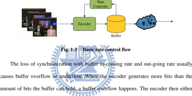
The task of controlling output bit rate by selecting an appropriate quantization parameter for each coding unit is performed by the rate control module. The goal of rate control is to keep the generated bit rate within the constrained bandwidth while achieving maximum video quality uniformly. A simple approach of rate control is shown in Fig. 1-3. Basically, the encoder buffer smoothes out the bit rate so that the averaged output bit rate matches the channel bit rate.

The loss of synchronization with buffer in-coming rate and out-going rate usually causes buffer overflow or underflow. When the encoder generates more bits than the amount of bits the buffer can hold, a buffer overflow happens. The encoder then either re-encodes the current frame with coarser QP or simply drops it (frame skip) to avoid the overflow. A buffer underflow is the situation while there is no bit available in the encoder buffer. It wastes the available channel bandwidth. By monitoring the status of buffer, the rate controller can adjust the quantization parameters, which affects the output bit rate, to prevent the buffer from overflow and underflow.

1.1.1 The Chicken Egg Dilemma for H.264 Rate Control

Fig. 1-2 (a) Variable bit rate vs. (b) Constant bit rate

Buffer Rate

Controler

Encoder

(14)



, | ,





, |





, |



Motion i i i i i i

J MB MV QP



D MB MV QP  



R MB MV QP (1.1) where MB_i and MV_i stand for the ith macro block (MB) and the motion vector (MV) of ith MB in the current frame, respectively; λ denotes the Lagrangian multiplier which depends on

 12 3

0.85 2QP



_ _ 

(1.2) According to (1.1) and (1.2), the cost calculation for each MV of the current MB takes QP as an important input parameter.

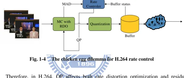
Therefore, in H.264, QP affects both rate distortion optimization and residual quantization. In this way, the statistical information of the residual frame, such as mean absolute difference (MAD), varies with the QP adjustment, and the QP decision is also influenced by the statistical information. As shown in Fig. 1-4, the rate control unit requires the MAD value from RDO to determine the QP value, but the RDO procedure also needs QP as an input parameter. This is the chicken egg dilemma for H.264 rate control.

1.1.2 Main Criteria of Rate Control

Rate control algorithms concentrate on keeping the encoded video quality as consistent and excellent as possible for each frame and constraining the bit rate within limited bandwidth. For grading rate control algorithms, there are four main criteria of

Buffer status Buffer Rate Controler QP Quantization MC with RDO MAD

(15)

rate control:

A. Mismatch between the target bit rate and the output bit rate.

Because the main purpose of rate control is to constrain the output bit rate within the target bit rate, the mismatch between both should be minimized.

B. Average PSNR of whole sequence.

The generated video quality should be at the highest possible level for a better watching experience.

C. Standard deviation of PSNR between frames.

This criterion implies the quality variation of the video produced by the rate control algorithm. A good rate control should keep the deviation low, i.e., keep the quality variation small.

D. Maximum buffer fullness.

A lower maximum buffer occupancy implies that a small buffer is sufficient for preventing from buffer overflow. Further, a small buffer only takes few buffer delay while transmission. A good rate control algorithm should minimize the maximum buffer fullness.

1.2 Introduction to H.264 Intra-coded Frames

H.264 exploits both temporal and spatial redundancy to increase its coding gain. It supports intra prediction mode to exploit the spatial domain correlation which helps reduce the residual energy of intra frames.

(16)

1.2.1 H.264 Intra Compression

H.264 utilizes the intra prediction to reduce the spatial redundancy within frames. Fig. 1-5 shows the prediction options of 4x4 block intra prediction. Each pixel in the current 4x4 block is predicted from the neighboring reconstructed pixels, where nine prediction modes can be selected by the encoder, and the residue between the current block and the predicted block will be quantized for entropy coding. The key to the success of intra coding on improving the performance is that the entropy of the residual block is much less than the original block. Hence, the coding gain after intra prediction will be significantly superior.

1.2.2 H.264 Intra-only Profiles

In the seventh edition specification of H.264, there are three new profiles, e.g.,

High 10 Intra, High 4:2:2 Intra, and High 4:4:4 Intra, which are designed for

professional applications. For the reason that the intra-only profiles does not exploit the temporal correlation, there is no temporal dependency between consecutive frames. It is more convenient for editing and parallel processing, even less error propagation. Table 1-1 summaries the differences between intra-only scheme and the standard GOP compression. Because of the features of intra-only compression, it is greatly appropriate for the high-end applications.

(17)

Table 1-1 Comparison between Intra-only and GOP compression[10]

1.3 Motivation

Rate control aims at providing highest possible video quality while satisfying the limited bandwidth. Although various rate control algorithms have been proposed for H.264 (see Chapter 2), most of them focus on inter coding instead of intra coding, even the output number of bits of an intra coding frame is much higher than that of an inter frame. It is also more possible that the intra coded frame causes buffer overflow when the generated bits exceed the amount of bits that buffer can hold.

Intra-only Compression GOP Compression

Compression scheme

Bit rate saving Smaller Use spatial

correlation only

Greater Use spatial and temporal correlations

Process delay Smaller 1 frame Greater Multiple frames

Edit easiness Easier frame by frame More difficult GOP

Error

propagation

Smaller Max. 1 frame Greater Multiple frames

Parallel processing

Easier Frame

independent

(18)

In the H.264 original rate control algorithm[11], the QP for each I-frame is decided by the average QP of all coded P-frames in the previous GOP. This approach does not take the buffer status and the frame complexity into consideration, and usually allocate too much bits for the I-frame, which degrades the video quality of the following P-frames due to insufficient bits. In addition, because the intra coded DCT coefficients are not Laplacian distributed, the quadratic model which is used to predict the relation between bit rate and quantization parameter is not appropriate for intra frames.

We also observed that the abrupt scene change usually results in buffer overflow due to the fact that most of MBs in the scene change frame are intra coded. It often

(a)

(b)

(c)

Fig. 1-6 (a) Bits, (b) PSNR and (c) the percentage of intra coded MB for the qcif sequence Akiyo-Foreman which cascaded at 50th frame, and the GOP size is 40

0 5000 10000 15000 0 50 100 B its Frame number 25 30 35 40 0 50 100 PS N R Frame number 0 50 100 0 50 100 In tr a M B (% ) Frame number

(19)

produces more bits than the target bits and degrades the visual quality of the following frames. Fig. 1-6 illustrates the fact mentioned above. In Fig. 1-6(c), the percentage of intra coded MBs at the scene change frame 50th is 100% which means all the MBs are encoded with intra mode. Fig. 1-6(a) and (b) shows the output bits of the scene change frame are much more than those of other frames and the PSNRs of the following frames are degraded until the start of the next GOP.

Since most existing rate control algorithms for H.264 cannot handle the intra frames and scene change frames well, we need to find out a new scheme to determine the QPs for both kinds of frames. Instead of using the average QP of P-frames in the previous GOP, in this thesis, we propose an improved rate control algorithm that take frame complexity into consideration to decide proper QPs for the both types of intra frames.

The remainder of this thesis is organized as follows: Chapter 2 introduces the related researches about rate control issue. Chapter 3 presents the proposed rate control scheme for Intra-only compression and Chapter 4 for GOP compression. Chapter 5 provides the simulation results compared to other rate control schemes. Finally, Chapter 6 concludes this thesis.

(20)

Chapter 2 Related Works

Rate control techniques have been studied intensively for many standards. The challenge of rate control in video encoding is to determine an appropriate quantization parameters to achieve the best video quality within the given application constraints. In this chapter, we will introduce the most famous rate control algorithm which is adopted in the official reference coding software of H.264[12] and other improved schemes for H.264 intra rate control.

2.1 G012 Rate Control for H.264

Li et al. proposed an one pass rate control algorithm, JVT-G012[11], which used the rate-quantization (R-Q) quadratic model in the standard MPEG4 rate control, and introduced the linear mean absolute difference (MAD) prediction model to solve the dilemma that we have mentioned in the previous chapter. Due to its efficiency, this scheme was adopted by JVT in the latest H.264 reference software.

2.1.1 Terminology

Before we introduce this algorithm, there are three terminologies we have to mention first.

A. Definition of A Basic Unit

Suppose that a frame is composed of N_mbpic macroblocks (MBs). A basic unit is defined as a group of continuous MBs which is composed of N_mbunit macroblocks where N_mbunitis a fraction of N_mbpic. Denote the total number of basic units in a frame by N_unit, which is given by

(21)

picunit unit mbunit N N N  (2.1)

A basic unit can be selected as a frame or some consecutive MBs. Note that, a smaller basic unit is needed in some low-delay applications which require stricter buffer regulations, less buffer delay, and better spatially perceptual quality. However, it is costly at low bit rate since there is additional overhead if the quantization parameter is varying frequently within a frame. On the other hand, by using a bigger basic unit, a higher PSNR can be achieved but the bit fluctuation is also larger.

B. Linear Model for MAD Prediction

MAD is the mean absolute difference between the reference frame and the current frame which describes the residue information and is given by

 

1 1









0 0 1 , , , H W i j MAD x y C x i y j R x i y j HW      



     (2.2)

where C and

R

stand for the original and referenced pixel, respectively.

In order to solve the chicken egg dilemma in H.264 rate control, the linear model is used to predict the MADs of the basic units in the current frame by using the MADs of the co-located basic units in the previous frame. The linear prediction model is then given by

1 2

pb cb

MAD  a MAD a (2.3)

where a₁ and a₂ are two coefficients of the prediction model; MAD_pb and MAD _cb

(22)

in [13][14]. Assume that the source statistics satisfy a Laplacain distribution

( ) where

2

x

P x 



e     x (2.4)

and the distortion measure is defined by, D x x( , ) x x , where

x

is the original sample and x is the reconstruction of

x

. Then, a closed solution for R-D function was derived as min max 1 1 1 ( ) ln where 0, , 0 R D D D D D



   _ _       (2.5)

Based on the R-D function, a quadratic rate-control model was proposed in [13] as

1 2 2 X X R QP QP   (2.6)

where R is the target number of bits used for encoding the current frame, and X₁ and

2

X are model parameters which are updated by linear regression method from previous coded information.

Lee et al.[14] improved the model with content scalability and achieved more accurate bit allocation within limited target bits. The improved model has been adopted as a part of the MPEG4 standard, and known as MPEG4 Q2 algorithm. The quadratic rate distortion model is defined by

1 2 2 MAD X MAD X R H QP QP      (2.7)

where H is the number of bits used for the header, the motion vectors, and other non-texture information. Here, MAD is used to measure the coding complexity for accomplishing the scalability of this model.

2.1.2 Overview to G012 Rate Control

(23)

GOP layer; 2) frame layer, and 3) basic unit layer. There are two sub-problems, bit allocation and QP determination, for each layer.

In GOP layer rate control, it calculates the total bits R_r for all non-coded frames within the current GOP, and selects the QP for the starting I-frame. In the beginning of each GOP, the total number of bits is computed as follows

r GOP c r u R N B F    (2.8)

where

u

is the channel bit rate; F_r indicates the frame rate; N_GOP denotes the number of frames in a GOP, and B_c is the occupancy of the buffer after coding the previous frame. In the case of constant bit rate, R_r is updated frame by frame as

r r

R R b (2.9)

Fig. 2-1 The G012 rate control diagram

GOP layer

Bit allocation for the GOP

Calculate the intra QP for the GOP

Frame layer

Bit allocation for the frame Calculate the QP for the frame

Basic unit layer

Bit allocation for the basic unit Calculate the QP for the basic unit

(24)

determined as the average QP of the P-frames of the previous GOP. Summarily, the starting QP is selected as follows

1 1 2 , 2 3 3 4 , 40 30 , 20 10 I first r pixel I other p bpp l l bpp l u QP where bpp l bpp l F N l bpp l SumQP QP N      _ _   __ _  _ _ _  _  _ _ _       (2.10)

where N_pixel is the number of pixels within a frame; N_p indicates the number of P-frames of a GOP, and SumQP stands for the summation of QPs of all P-frames of the previous GOP. l_i, 1 i 4, are the predefined thresholds.

The approach of frame layer involves distributing the GOP budget among the frames and determines the QP of each frame to achieve the allocated budget. The target number of bits of ith P-frame in the current GOP is determined as





ˆ ₁

i i i

R    



R



R (2.11)

where



is a weighted constant; Rˆ_i and R_i are defined as

ˆ r i remain R R N  (2.12)





i i i r u R Tbl V F



    (2.13)

where N_remain is the number of non-coded frames in the current GOP;



is a constant, and Tbl_i and V_i are the target buffer level and the virtual buffer fullness of the ith frame, respectively.

After accomplishing the bit allocation, the linear MAD prediction model (2.3) and the quadratic rate distortion model (2.7) are utilized to determine the QP of the current

(25)

frame, then RDO procedure is performed for mode decision. At the last, the parameters of the quadratic model, and those of the MAD prediction model are updated based on the coding results.

If frames are not selected as basic units, basic unit layer rate control should be performed after frame layer bit allocation. In basic unit layer, it is almost the same as that in frame layer. It predicts MADs of all basic units in the current frame by equation (2.3) and calculates the target number of bits of them by

2 , , 2 , unit i pred i c remain N j pred j i MAD b R MAD   



(2.14)

where R_{c remain}_, is the remaining target number of bits of current frame; MAD_{i pred}_,

stands for the predicted MAD of ith basic unit in the current frame. Then, the quadratic model (2.7) is proposed to determine the QP of the current basic unit.

2.2 Cauchy Density based Rate Control for H.264

Knowledge of the probability distribution of discrete cosine transform (DCT) coefficient is important in the design and optimization of rate control algorithms. In the early studies [15], the coefficients are conjectured to have Laplacian distribution. In [16], Kamaci et al. proposed a better solution using a Cauchy probability density function (pdf) for DCT coefficients estimation. As shown in Fig. 2-2, Cauchy model actually outperforms traditional Laplacian model in both intra and inter coded frames.

(26)

Kamaci et al. further presented the Cauchy density based rate estimation models by approximating the entropy function of quantization. The rate model was applied in frame layer to determine the QP of each frame based on the given target number of bits of current frame,

R

.

Their Cauchy based rate estimation models is

b

R a QS (2.15)

where QS is the quantization step;

a

and b are model parameters which depend on the content of the coding sequence and different types of coding mode, i.e., I-, P-, and B-frames. Then, the QS is determined as following

b R QS

a

 (2.16)

Finally, the QP used for RDO can be calculated by

2

6 log ( ) 4

QP  QS  (2.17)

where denotes the rounding operation.

(27)

2.3 Frame Complexity based Intra only Rate Control

Based on Kamaci et al.’s rate estimation model, Jing et al.[17] proposed an improved model which is applied on intra frames and has sufficient adaptability to the varying of intra frame complexity.

In their proposed algorithm, they defined the complexity measure of intra frames as the average gradient per pixel of the frame. The calculation of gradient complexity is defined by 1 1 , 1, , , 1 0 0 1 M N i j i j i j i j i j G I I I I M N          _    _  



 (2.18)

where M and

N

are the horizontal and vertical dimensions of the frame, respectively; I_{i j}_, denotes the luminance value of the pixel at the location of

 

i j, .

(a) 0.6 0.8 1 1.2 1.4 8 10 12 14 16 18 20 In tr a co d e d b its x 10000

Gradient per pixel

3 3.5 4 tr a co d e d b its x 1000 0

(28)

They observed that the number of coding bits of an intra coded frame is highly correlated with its gradient value, as shown in Fig. 2-3. From the linear correlation between these two factors, they assumed that for a fixed QP, the output number of bits of one intra frame is proportional to the value of its average gradient per pixel. Based on the assumption, they revised Cauchy rate estimation model as follows

b

R  G a QS (2.19)

where b is a constant which is set to -0.8 and a is updated frame by frame as





0 0 0 1 1 1 1 0 1 b k k k b k k R k G QS a R a otherwise G QS



     _  _            (2.20)

After frame layer bit allocation, QS can be calculated by (2.19), and QP can be derived from (2.17).

2.4 Intra Frame Bit Allocation Algorithm

Sun et al.[18] exploited prediction and feedback control to achieve accurate rate control while maximizing the picture quality and smoothing buffer fullness. Their algorithm estimates the bit budget for the I-frame of ith GOP based on its global coding complexity with the following equation

, , Intra i i r Intra i Inter p W R R W W N     (2.21)

where N is the number of P-frames in GOP; _p W_Inter is the weighting of inter coded frames which is set to 1. W_Intra stands for the weighting of intra coded frames which is calculated as follows

(29)

( ), 1 ( ), 1

( ), 1 ,

( ), 1

avg Inter i avg Intra i

PSNR PSNR avg Intra i Intra i avg Inter i Bit W e Bit           _ _    (2.22)

where Bit_{avg Intra i}₍ _{), 1}_ and PSNR_{avg Intra i}₍ _{), 1}_ are the average number of bits and PSNR of the I-frame in the previous GOP, respectively, Bit_{avg Inter i}₍ _{), 1}_ and PSNR_{avg Inter i}₍ _{), 1}_

denote those of P-frames, and



is a model parameter which is set to 8 in their experiments. In equation (2.21), the target number of bits of the I-frame in the current GOP is determined by the intra weighting value which relies on the coding results of the previous GOP.

They also proposed a novel buffer controller based on the proportional integral derivative (PID) technique used in automatic control systems, and used (2.7) to determine QP.

2.5 Adaptive Distortion based Intra Frame Rate Control

Yan et al.[19] presented an adaptive distortion based intra rate estimation (ADIE) algorithm for H.264/AVC rate control. In this algorithm, a new rate control model is established according to the distortion which is predicted by taking image complexity, buffer status and scene change into considerations. From the quadratic rate model (2.5), they supposed the output bit rate is related to the output MSE, and is given by

1 ln R MSE



   _ _ _ (2.23) MSE

(30)

Based on the above observation, they proposed that the relation between QS and MSE can be approximately modeled as

QS  



MSE



(2.24)

where the value of



can be obtained after coding the first I-frame, and



is a constant. Finally, their proposed MSE prediction model which based on gradient complexity and buffer status is

, 1 1 1 1 i pred i i i G MSE MSE MG BR



       (2.25)

where MG is the mean gradient value of previous I-frames in this sequence, and



is a model constant. BR_i is the current buffer fullness ratio derived by

i

BF BufferSize where BF_i is the buffer fullness after encoding the ith GOP. After the MSE prediction using (2.25), the model (2.24) is employed to determine the appropriate QS value.

2.6 Summary

In the above sections, we have introduced several researches for H.264 rate control and intra coded frame rate control. However, they still have some problems which can

(31)

be organized as follows:

A. Without Dealing with Scene Change Intra Frames

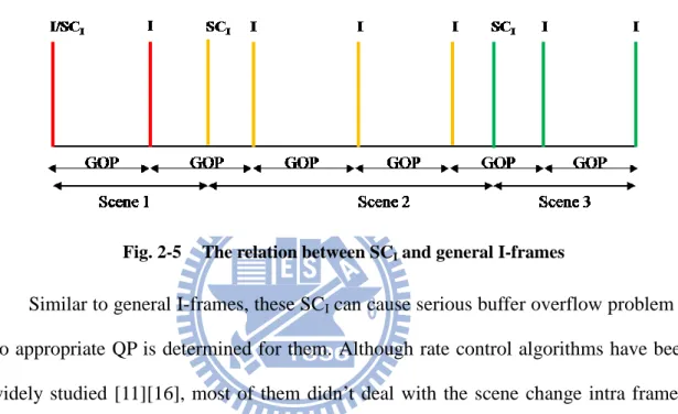
Due to that all MBs within a scene transition frame will be intra coded as observed in Fig. 1-6, we regard such a frame as a special kind of intra frame, called scene change intra frame (SCI). The locations of SCI frames and general intra frames in a video

sequence can be illustrated by Fig. 2-5.

Similar to general I-frames, these SCI can cause serious buffer overflow problem if

no appropriate QP is determined for them. Although rate control algorithms have been widely studied [11][16], most of them didn’t deal with the scene change intra frames. Yan et al.[19] had their mechanisms to detect scene change. However, they calculated the QP by using equation (2.10) which is not appropriate.

B. Poor QP Determination for General Intra Frames

In G012, the QP of each I-frame is decided by the average QP of all coded P-frames in the previous GOP. This simple approach which does not take frame complexity and buffer fullness into considerations may suffer from buffer overflow.

(32)

C. No Accurate Rate Quantization Model for Intra Frames

The quadratic model (2.7) is designed for inter coded frames whose source statistics are assumed satisfying Laplacain distribution. However, this assumption is inappropriate to intra coded frames. Jing et al.[17] proposed a novel rate quantization model for intra frames, but the parameter,

a

used in their model cannot be estimated precisely. In order to determine this parameter, they employed an update procedure which assumes that its value is stationary frame by frame. However, this assumption is not always true as illustrated in Fig. 2-6 where the value of

a

in the figure varies frequently.

Fig. 2-6 The value of parameter a from akiyo sequence

124000 126000 128000 130000 1 31 61 91 121 151 181 211 241 271 a Frame number

(33)

Chapter 3 Proposed Rate Control Algorithm for

Intra-only Compression

In this chapter, we present the proposed rate control algorithm for Intra-only compression. As mentioned in section 2.6, there are two kinds of intra frames should be dealt with. We first describe a Lagrangian-optimization based rate control scheme for intra frames, and then a gradient complexity based scheme is proposed for scene change intra frames (SCI frames).

For Intra-only compression, since all frames are intra coded, there is no need to consider the difference between coding modes. A simple and efficient bit allocation for the current general I-frame is

remain t r R R N  (3.1)

where R_remain is the available bit budget for remaining frames within the current GOP, and N_r is the number of remaining frames.

3.1 Lagrangian-Optimization based QP Determination for

Intra Frames

The proposed Lagrangian-optimization based rate control scheme is for QP determination of intra frames. First, we define the Lagrangian cost function as

(34)

It is obvious that the higher the cost value J QP

 

is, the better tradeoff between quality and rate can be obtained. In this section, PSNR

 

, R

 

, and



, are introduced first. Then, a QP determination algorithm based on equation (3.2) for general intra frames is proposed.

3.1.1 Taylor Series based Rate-QS Model

In section 2.6-C, we have mentioned the drawback of Jing’s intra rate quantization model. In order to solve this problem, we modified the equation (2.19) by defining the normalized bit rate of ith frame, R_{norm i}_, as follows

, b i norm i i R R aQS G   (3.3)

We gather statistics of R_norm from different frames with all QS in intra coding mode. Fig. 3-1 and Fig. 3-2 show the curves of R_norm

 

x for the first five frames in

foreman and akiyo sequences, respectively. It indicates that the R_norm

 

x curves in neighboring frames or frames in the same scene are closely identical. In other words, the

 

norm

R x curve of the current intra frame can be predicted from that of the previous intra frame if it is available.

Fig. 3-1 The curves between R and QS of Foreman

0 2000 4000 6000 8000 10000 12000 14000 16000 0 50 100 150 200 250 Rn or m QStep

(35)

In fact, there is one single point available in the curve of the previous intra frame because the QS used and the number of bits encoded for the previous intra frame can be obtained after its encoding procedure. Taylor series theory[22] indicates that any infinitely differentiable function, f x

 

, can be represented as an infinite sum of terms calculated from all the values of derivation at a single point. Based on Taylor series theory, the formula of R_{norm i}_, can be represented as1

 

















, 2 , , , 1! 2! b norm i norm i i norm i i norm i i i i R x aQS R QS R QS R QS x QS x QS         (3.4)

where R_norm

 

QS_i and R_norm

 

QS_i can be derived from

Fig. 3-2 The curves between Rnorm and QS of Akiyo 0 2000 4000 6000 8000 10000 12000 14000 16000 0 50 100 150 200 250 Rn or m QStep

(36)

 



_{ }

 



 



 



 

1 2 2 ( 1) 2 norm b norm norm norm norm norm d R QS R QS R QS b a QS b d QS QS d R QS R QS R QS b b QS d QS   _ _                   _{   } _  _ _  (3.5)

According to equations (3.3), (3.4), and (3.5) as well as the property that successive frames has identical R_norm curves, the proposed Taylor series based rate-QS model is









, , 1 2 , 1 1 , 1 1 , 1 1 1 ( ) ( ) ( ) ( ) ( ) 1! 2! i i norm i i norm i norm i i norm i i i norm i i i R x G R x G R x R QS R QS G R x QS x QS                  _     _  









, 1 , 1 2 2 1 1 , 1 1 1 ( 1) 1! 2! norm i norm i i i i norm i i i R R b b b QS QS G R x QS x QS                             _     _       (3.6)

where b is a constant set to -0.76 in this thesis; R_{norm i}_,_₁ and QS_i_₁ are the normalized number of bits encoded and the QS used in of the previous intra coded frame, respectively. Note that, R_norm_,0 and QS₀ can be obtained after the coding procedure of the first intra frame.

Two experiments for the comparison between the proposed model and Jing’s model (2.19) were conducted and the results were shown in Fig. 3-3. Note that, prediction error is calculated by equation (3.7). It is observed that the proposed model can achieve more accurate prediction, especially for the beginning frames. Compared with Jing’s rate quantization model, the proposed Taylor series based model is more reliable due to its independence to the unstable model parameter,

a

. The proposed model can reduce the bit rate prediction error by up to 73%.

, , 100 actual i predict i predict Bits Bits Error Bits    (3.7)

(37)

(a)

(b)

Fig. 3-3 Prediction error comparison of proposed model and Jing’s model. Analysis from (a) Foreman@QCIF-512kbps and (b) Mobile@QCIF-512kbps

0 2 4 6 8 10 12 14 2 12 22 32 42 52 62 72 82 92 P re d ic t er ro r (%) Frame number

Jing ( Average error 2.05% ) Proposed ( Average error 1% )

0 5 10 15 20 25 30 2 12 22 32 42 52 62 72 82 92 P re d ic t er ro r (%) Frame number

(38)

PSNR by the following model

PSNR

 

m QP k



(3.8)

where

m

and k are parameters relying on the content of sequence.

Fig. 3-4 also shows the slope,

m

, of each curve is different from others. The tendency of the slopes is related to frame complexity: the larger frame complexity , the more titled slope. After analyzing data from over 3000 intra coded frames, we realize the relation between the slope and the gradient based frame complexity, G, is also linear. Fig. 3-5 shows this relation. Based on the observation, we modelize the relation of

m

and gradient based frame complexity, G, with a linear training line.

During our model parameter updating procedure, the value of

m

and k are

Fig. 3-4 The relation curves between PSNR and QP of several sequences

Fig. 3-5 The relation between model parameter, m and frame complexity, G

15 20 25 30 35 40 45 50 55 60 5 10 15 20 25 30 35 40 45 50 P S N R QP

claire akiyo carphone foreman silent

salesman news coastguard container mobile

y = -0.0064x - 0.6622 R² = 0.9603 -1 -0.9 -0.8 -0.7 -0.6 0 5 10 15 20 25 30 35 40 45 m G

(39)





1 1 1 1 2 i i i i i i i G m m k PSNR m QP





_                (3.9)

where PSNR_i₁ and QPi1 are from the previous intra coded frame;



 0.0064

and



 0.6622 are used for QCIF sequences.

34 34.5 35 35.5 36 0 5 10 15 20 25 30 35 40 45 50 55 60 65 70 75 80 85 90 95 P S N R Frame number

Real Predicted (Average error 0.18%)

40 40.5 41 41.5 42 P S N R

(40)

To demonstrate the accuracy of the proposed gradient complexity based PSNR-QP model, Fig. 3-6 shows the experimental results, where real PSNR value and predicted PSNR value of each frame in the Foreman sequence are presented. It clearly illustrates the proposed model is reliable because the predicted PSNR curve closely fits the real one.

3.1.3 Estimation of λ

In Lagrangian cost function (3.2), the Lagrangian multiplier,



_{, plays an} important role to balance the weight of visual quality and departure from the target bit rate. If the value of



is too small, the second term of the cost function has no influence against to the first term. If it is too large, the result is severely affected by the target bit rate departure, so the cost function cannot determine the best QP for intra coded frames.

In order to derive a fair Lagrangian multiplier, we substitute the proposed PSNR-QP model (3.8) and Jing’s Rate-QS model2 (2.19) into the cost function which can be written as

 





( ) _t b t J QP PSNR QP R QS R m QP k G aQS R



          





₂  6 4 b QP t m QP k



G a R          (3.10)

According to Lagrangian optimization method, the optimized solution happens while  J QP0. It indicates that



under optimized condition can be derived with3

2

Due to the complexity of the proposed rate-QS model, we adopt Jing’s model to derive  for simplicity.

(41)

 

( 4) 6 ( 4) ( 4) 6 6 ( 4) 6 0 ( ) ( ) , 1 log 2 2 6 19.96 19.96 2 2 ( ) ( ) 19.96 , 2 t t b QP b b QP b QP b b QP R QP R PSNR QP J QP QP QP PSNR QP R QP m if R QP R QP QP abG m m QS abG Rb PSNR QP R QP m QS otherwise QP QP Rb



        _ _{ } _       _ _ _  _ _            _ _    _{ }  _       _  _ _          

Finally, the value of



can be calculated with

 4 6 19.96 2 b b QP m QS Rb



   _  (3.11)

while the estimated number of bits is larger than the number of target bits. On the other hand, while the estimated number of bits is smaller than the target number of bits,



is

 4 6 19.96 2 b b QP m QS Rb



   _  (3.12)

3.1.4 QP Determination Method for Intra Frames

After the introduction of the above three main components in the cost function, we propose a novel QP determination algorithm for intra frames. To obtained the best QP, we can substitute all possible QPs into Lagrangian cost function (3.2) and calculate the cost value of each QP. The optimized QP is the one with the largest cost value. In order to take PSNR deviation constrain into consideration, we propose that only QPs within

(42)

3.2 Gradient Complexity based QP Determination for

Scene Change Intra Frames

The gradient complexity based rate control scheme for scene change intra frames (SCI frames) is proposed in this section. First, we present a gradient based scene change

detection algorithm, and then the QP determination method is described.

3.2.1 Gradient based Scene Change Detection

In order to prevent the buffer overflow problem caused by SCI frames, a scene

change detection algorithm is essential. If a remarkable difference between consecutive frames can be detected by a appropriate metric which describes the frame characteristic perfectly, a scene transition can be declared whenever that metric exceeds a given threshold.

Various such metrics have been studied over years. In [5], Kim et al. have classified these frame complexity measures into four categories and suggested that the gradient based method is more reliable. According to Kim’s research, we propose a gradient based scene change detection algorithm.

First, the pixel gradient at the location of

( , )

i j

in the nth frame is defined as

 

,

  

, , 1



  

, 1,



n

g i j  I i j I i j  I i j I i j (3.13) where I i j

 

, denotes the luminance value of the pixel at the location of

( , )

i j

. And

(43)

the frame complexity of nth frame is measured as

 

1 1 0 0 1 , H W n i j G g i j H W        _ _  



 (3.14)

where W and H are the horizontal and vertical dimensions of the frame, respectively. Then, the average gradient difference of the co-located pixel between consecutive frames, named mean difference of gradient ( MDOG ), is given by

 

1

 

1 1 1 , , H W n n n i j MDOG g i j g i j WH    



 (3.15)

Intuitively, the value of MDOG should be distinguishable while the scene change happens. Fig. 3-8 shows the MDOG values of a cascaded test sequence which is composed of Trevor, Stefan, Silent, and Coastguard sequences. There are three scene change frames at 50th, 100th, and 150th, respectively. Although MDOG values at three scene change frames are relatively higher than their respective neighboring frames, a high-motion sequence would get an over estimated MDOG of non scene change frames due to its fast action. The second cut of the cascaded sequence, Stefan, is a classical high-motion example.

Fig. 3-8 MDOG value of the QCIF sequence Trevor-Stefan-Silent-Coastguard

0 10 20 30 40 0 50 100 150 200 M D OG Frame number

(44)

1

n n n n

FD  MDOG MDOG_ MDOG (3.16)

Note that, the second term, MDOG_n_{, is a scalar used to dynamically enhance the} effect of the first difference term while current frame is unlike the previous one. Fig. 3-9 shows

FD

values of eight cascaded test sequences and it indicates a threshold of 35 is a good choice to decide whether a scene transition occurs. Note that, the starting I-frame which is the first frame of the sequence is considered a scene change frame.

To demonstrate the correctness of the proposed scene change detection algorithm with

FD

threshold 35, experiments were conducted for two advertisement sequences with many scene transitions. The results are shown in Table 3-1 where N_SC is the number of scene change frames; N_C is the number of correct detection; N_m presents the number of miss detection, and N_f stands for the number of false alarms. It is obvious that most of scene change frames of both sequences are detected, and the number of false alarms is low.

Fig. 3-9 FDs of eight QCIF cascaded sequences when the threshold is set to 35

0 100 200 300 400 500 600 700 800 900 0 50 100 150 200 FD Frame number B1 B2 B3 B4 D1 D2 D3 D4 35

(45)

Sequences Frames N_SC N_C N_m N_f

AD1 898 19 15 4 1

AD2 900 20 18 2 9

Table 3-1 Detection correctness of two advertisements

The proposed scene change algorithm is efficiency due to the low complexity gradient operation, and the value of pixel gradient is re-useable in the frame complexity measurement, shown in equation (3.14).

3.2.2 Gradient Complexity based Rate-QS Model

Because of the scene transition, the information from previous coded frames is not useful to predict the result of current SCI frame. In order to solve the buffer overflow

problem caused by SCI frames, we propose a gradient complexity based rate-QS model

for SCI frames. The proposed model is based on Jing’s rate-QS model (2.19), but it only

takes information of current frame as predictor.

After analyzing data from over 3000 intra coded frames, we realize the relation between the gradient based frame complexity, G and the term of G a is closely

Fig. 3-10 The relation curve between G and G*a

y = 6022.1x + 88520 R² = 0.7513 50000 150000 250000 350000 450000 0 10 20 30 40 50 G * a G

(46)



6022.1,88520, 0.76



. According to the improved model (3.17), QS can be calculated with t b i i R QS G





   (3.18)

, and QP can be derived from (2.17).

To show the effects of taking account for scene changes in the rate control, Fig. 3-11 shows the prediction error for intra-only compression on a cascaded sequence with scene changes at frames 10, 20, 30, and 40. The rate control methods used for comparison include: Jing’s method, the proposed rate control method (the proposed method), the proposed method without scene change consideration (proposed w/o SC). The prediction error is calculated by equation (19). In Fig. 3-11, it is obvious to see that, compared with other two methods, the proposed method is more accurate on bit-rate prediction at the scene change frames.

Fig. 3-11 Prediction error comparison from a cascaded scene change sequence.

0 2 4 6 8 10 12 14 16 18 20 0 5 10 15 20 25 30 35 40 45 50 P re d ic t er ro r (%) Frame number

(47)

3.3 Description of the Proposed Rate Control Algorithm for

Intra-only Compression

With the scene change detection method, bit allocation for intra frames, and QP determination algorithms for both general intra frames and SCI frames, the detailed

block diagram of the proposed rate control algorithm for Intra-only compression is shown in Fig. 3-12. We summarize it with the following five steps.

Step 1. Calculate the gradient frame complexity, G and the frame distance,

FD

of the ith frame using equation (3.14)－(3.16).

Load One Frame

Calculate Gradient Complexity & Frame Distance

Target Bit Allocation

Scene Change Frame ?

Scene Change Intra Rate Control

Yes

Non Scene Change Intra Rate Control

No RDO Finish Sequence ? No Yes Update Model Parameters: λ, m, k, R, R`, R``

Fig. 3-12 Flow charts for Intra-only compression

(48)

in section 3.1.4. On the other hand, calculate a appropriate QS using (3.18) and derive QP with (2.17) for scene change intra frames.

Step 4. Perform H.264 RDO for mode decision and the following coding procedures with the determined QP. After RDO procedure, update model parameters such as

, ,

, , ,m k R_{norm i},R_{norm i}



 , and R_{norm i} _, with the coding result of the ith frame. Step 5. Go to Step 1 until the end of the sequence.

(49)

Chapter 4 Proposed Rate Control Algorithm for

GOP Compression

For GOP compression, there are two kinds of frames, intra coded and inter coded frames. QP determination for intra coded frames is the same with that mentioned in the previous chapter. On the other hand, we adopt G012 algorithm for inter frame rate control. Because of the difference between both kinds of frames, we first propose a novel target bit allocation scheme for intra frames. Then, the overall description of the proposed rate control algorithm for GOP compression is presented.

4.1 Target Bit Allocation for Intra Frames

For GOP compression, the starting I-frame usually needs more bits and better quality for the following P-frames. The bit allocation for the first I-frame is calculated as ,0 t r u R F



  (4.1)

where R is the target bit of I-frame in the 0_t_,0 th GOP;

u

is the channel bit rate; F_r

stands for the frame rate, and



is a constant which is set to 8 experientially.

Since there are intra and inter coded frames in GOP compression, the relation between both is important for bit allocation. Yu’s intra bit allocation formulas, (2.21) and (2.22) have several factors: average number of bits used in encoding previous

(50)

, , , , , Intra i t i remain i Intra i Inter i p W R R W W N



     (4.2) 1 1 2 2 3 1.8 1.6 < 1.4 < 1.2 G TH TH G TH TH G TH otherwise



   _    _  

where







TH TH TH₁, ₁, ₃



is the threshold set; R_{t i}_, is the target number of bits of I-frame in the ith GOP. W_Intra and W_Inter are the weighting of intra frames and inter frames, respectively.



is an adaptive scalar depending on the complexity of current frame, G_n, and the threshold of



. Wang et al.[21] proposed that the more complex sequences, the larger QP for the initial I-frame is required to obtain the best visual quality under the same bit rate.

In Fig. 4-1, it is observed that large QPs are required for the initial I-frame of high complex sequences such as Mobile; while relatively small QPs are required for that of low complex sequences such as News and Foreman. Note that,

BPP

is calculated by equation (2.10) and actual points are determined by trying all possible QPs and recording the best one which results in the best R-D point. Based on this observation,

Fig. 4-1 Relation curves between the best initial QP and bpp for News, Foreman, and

(51)

the scalar



is set adaptively, and the threshold set



is set as below



9.65,15.59,18.03





 for QCIF sequences.

4.2 Description of Proposed Rate Control Algorithm for

GOP Compression

Fig. 4-2 depicts the flow chart of the proposed rate control algorithm for GOP compression. It is similar with the original framework of G012, but QPs of both kinds of intra frames are determined by the proposed algorithm. We summarize it with the following five steps.

Load One Frame Calculate Gradient Complexity

& Frame Distance

Intra Target Bit Allocation Scene Change

Frame ?

Scene Change Intra Rate Control

Yes Normal P Frame Rate Control No RDO I Frame ? P Frame I Frame

Non Scene Change Intra Rate Control Intra Target Bit

Allocation Update Model

Parameters: λ, m, k, R, R`, R``

(52)

Step 1. This step is the same with the first step in Intra-only scheme.

Step 2. If current frame is I-frame, allocate target bits using equation (4.2) and determine QP with the method in section 3.1. Then, perform H.264 RDO with the determined QP.

Step 3. If current frame is P-frame, detect whether it is a scene change frame. If it is a SCI frame, determine QP with the method in section 3.2. If not, the QP is

calculated with the P-frame mode by G012 proposal. Then, H.264 RDO procedure is performed after the QP determination.

Step 4. The updating stage is the same with the 4th step in Intra-only compression. Step 5. Go to Step 1 until the end of the sequence.

基於拉格朗日最佳化針對 H.264 畫面內編碼的位元率控制演算法

國立交通大學

資訊科學與工程研究所

碩士論文