基於深度資訊之智慧型人形偵測系統設計

國 立 交 通 大 學

電控工程研究所

碩 士 論 文

基於深度資訊之

智慧型人形偵測系統設計

Intelligent Human Detection System Design

Based on Depth Information

研 究 生：陳咨瑋

指導教授：陳永平 教授

基於深度資訊之

智慧型人形偵測系統設計

Intelligent Human Detection System Design

Based on Depth Information

研

究 生：陳咨瑋 Student：Tzu-Wei Chen

指導教授：

陳永平 Advisor：Professor Yon-Ping Chen

國

立 交 通 大 學

電控工程研究所

碩

士 論 文

A Dissertation

Submitted to Institute of Electrical Control Engineering College of Electrical and Computer Engineering

National Chaio Tung University In Partial Fulfillment of the Requirements

For the Degree of Master In

Electrical Control Engineering June 2012

Hsinchu, Taiwan, Republic of China

基於深度資訊之

智慧型人形偵測系統設計

學生: 陳咨瑋 指導教授: 陳永平 教授

國立交通大學電控工程研究所

摘 要

近年來，由於人形偵測可應用的領域相當廣泛，因此受到重視且被深入的 研究與討論，例如居家照護、人機溝通、智慧型汽車等皆是。本篇論文提出以 Kinect 所產生的深度圖為基礎的智慧型人形偵測系統，除了提高人形偵測率外， 同時解決人形遮蔽的問題。整個系統分成三個部分：前景偵測、特徵擷取以及人 形識別。雖然人會有許多不同的姿勢，但主要都是以垂直分布的方式呈現並具有 一定的高度，根據此特性本系統先去偵測人形可能存在的區域，並且濾掉背景以 增快速度；之後藉由邊緣擷取和距離轉換來萃取人形特徵，用以增加辨識率；此 外畫面中的人形常因他人或物品之遮擋而只露出部分輪廓，為了解決這種遮蔽問 題，本系統並不直接偵測整個人形，而是先利用凹槽匹配法找出各個身體部位， 像是頭、身體、腳等，再利用類神經網路把各身體部位加以組合，並依此判斷是 否為人形。根據實驗結果，本系統確實可以快速地偵測出人形，同時解決遮蔽問 題，使偵測率提高至 90%以上，甚至高達 95%。

Intelligent Human Detection System Design

Based on Depth Information

Student：Tzu-Wei Chen Advisor：Prof. Yon-Ping Chen

Institute of Electrical Control Engineering

National Chiao-Tung University

ABSTRACT

This thesis proposes an intelligent human detection system based on depth information generated by Kinect to find out humans from a sequence of images and resolve occlusion problems. The system is divided into three parts, including region-of-interest (ROI) selection, feature extraction and human recognition. First, the histogram projection and connected component labeling are applied to select the ROIs according to the property that human would present vertically in general. Then, normalize the ROIs based on the distances between objects and camera and extract the human shape feature by the edge detection and distance transformation to obtain the distance image. Finally, the chamfer matching is used to search possible parts of human body under component-based concept, and then shape recognition is implemented by neural network according to the combination of parts of human body. From the experimental results, the system could detect humans with high accuracy rate and resolve occlusion problems.

Acknowledgement

本篇論文得以順利完成，首先必須感謝指導教授 陳永平老師的諄諄教悔， 使作者除了在研究及英文寫作上有長足的進步外，在為學處事態度上也有相當的 成長，僅向老師致上最高的謝意；同時也感謝 林進燈老師以及 楊谷洋老師等 口試委員的建議與指教，使論文得以更加完善。 其次，感謝實驗室的世宏、桓展學長在求學與專業研究的過程中給予適時的 建議及鼓勵，並提供許多寶貴的經驗，同時感謝實驗室同學榮哲、振方、崇賢、 孫齊以及學弟谷穎、宣峻、仕政、兆村為我兩年研究生的生活帶來許多的歡樂及 回憶，而我的論文也在與大家的相互激盪下，多了許多不同的靈感與面向，此外 也感謝大學同學振淵、奕晴、凱涵、青維、鈞凱，謝謝你們一路的相伴與支持。 最後，感謝我的家人在精神上的支持與鼓勵，還有生活上的照顧和關心，讓作者 能安心的投入研究並擁有美好的碩士生活。 謹以此篇論文獻給所有關心我、照顧我的人。 陳咨瑋 2012.6

Contents

Chinese Abstract ... i English Abstract ... ii Acknowledgment ... iii Contents ... iv List of Figures ... vi List of Tables ... ix Chapter 1 Introduction ... 1 1.1 Preliminary ... 1 1.2 System Overview... 3 1.2.1 Hardware Architecture ... 3 1.2.2 Software Architecture ... 4

Chapter 2 Related Works ... 6

2.1 Human Detection Methods ... 6

2.1.1 Foreground Segmentation ... 6 2.1.2 Feature Extraction ... 7 2.1.3 Human Recognition ... 8 2.2 Introduction to ANNs ... 10 2.3 Back-Propagation Network ... 13 2.4 Morphology Operations ... 16

Chapter 3 Intelligent Human Detection ... 19

3.1 ROI Selection ... 20

3.1.1 Histogram Projection ... 21

3.1.2 Connected Component Labeling ... 24

3.2 Feature Extraction ... 29 3.2.1 Normalization ... 29 3.2.2 Edge Detection ... 31 3.2.3 Distance Transformation ... 34 3.3 Human Recognition ... 36 3.3.1 Chamfer Matching ... 36 3.3.2 Shape Recognition ... 38

Chapter 4 Experimental Results ... 46

4.1 ROI Selection ... 46

4.2 Feature Extraction ... 51

4.2.1 Normalization ... 51

4.2.2 Edge Detection and Distance Transformation ... 53

4.3 Human Recognition ... 55

Chapter 5 Conclusions and Future Works... 60

List of Figures

Fig-1.1 Example of depth image ... 4

Fig-1.2 Software architecture ... 5

Fig-2.1 Examples of Haar-like features ... 8

Fig-2.2 Basic structure of ANNs ... 11

Fig-2.3 Multilayer feed-forward network ... 12

Fig-2.4 Neural network with one hidden layer ... 13

Fig-2.5 Example of dilation ... 17

Fig-2.6 Example of erosion ... 18

Fig-3.1 Flowchart of the intelligent human detection system ... 19

Fig-3.2 (a) Example of the depth image generated by Kinect (b) The image after dilation operation ... 20

Fig-3.3 Result of histogram computing of Fig-3.2(b) ... 22

Fig-3.4 Filtered result of Fig-3.3 ... 23

Fig-3.5 Example of top-view image ... 24

Fig-3.6 (a) Top-view image after dilation operation (b) The ROI image ... 24

Fig-3.8 Example of 4-pixel CCL (a) Binary image (b) Labeling

(c) Componentizing ... 26

Fig-3.9 (a) Result of CCL. (b) The corresponding regions in the depth image ... 27

Fig-3.10 Results of CCL and examples of occlusion judgment. (a) Non-occlusion (b) Frontal-occlusion (c) Left-occlusion (d) Right-occlusion ... 28

Fig-3.11 Example of perspective projection ... 30

Fig-3.12 (a) The original image (b) The result of ROI selection (c) Extracted region from ROI selection (d) The result of normalization ... 31

Fig-3.13 Example of Sobel operators ... 33

Fig-3.14 Result of edge detection ... 33

Fig-3.15 (a) Example of edge image (b) Result of distance transformation ... 34

Fig-3.16 Result of distance transformation ... 35

Fig-3.17 Example of Chamfer matching ... 37

Fig-3.18 Two different template sets. (a) Set-I (b) Set-II ... 38

Fig-3.19 Scheme of voting-based recognition ... 40

Fig-3.20 Structure of Set-I neural network ... 42

Fig-3.21 Set-I neural network ... 43

Fig-3.23 Set-II neural network ... 45

Fig-4.1 Results of ROI selection in the condition of different poses ... 47

Fig-4.2 Results of ROI selection in the condition of one human and one chair ... 48

Fig-4.3 Results of ROI selection in the condition of more than one human ... 49

Fig-4.4 Results of ROI selection in complex background ... 50

Fig-4.5 The same human standing in 1.6m, 2.0m, 2.4m, 2.8m, 3.2m and 3.6m from top to bottom.(a) Original depth images (b) The results of ROI selection (c) The extracted human regions. (d) The results of normalization ... 52

Fig-4.6 Comparison of the result of normalization. The human is originally standing at 1.6m, 2.0m, 2.4m, 2.8m, 3.2m and 3.6m from left to right ... 53

Fig-4.7 Result of edge detection and distance transformation in the condition of walking pose ... 53

Fig-4.8 Result of edge detection and distance transform in the condition of more than one human ... 54

Fig-4.9 Result of edge detection and distance transform in complex background ... 54

Fig-4.10 Result of edge detection and distance transformation in the condition of one human and one chair ... 55

Fig-4.11 Examples of test images in DP group ... 57

Fig-4.12 Examples of test images in OC group ... 57

Index of Tables

Table 1.1 Specification of Kinect ... 3

Table 4.1 TP, FP, FN, TN table ... 56

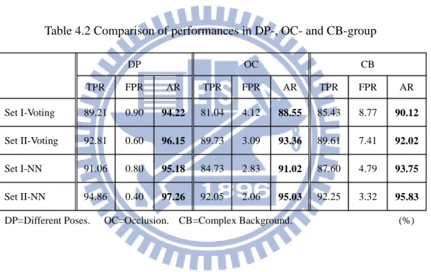
Table 4.2 Comparison of performances in DP-, OC- and CB-group ... 59

Chapter 1

Introduction

1.1 Preliminary

In recent years, the techniques for human detection in images or videos have been widely and intensively studied because they have a variety of applications in intelligent vehicles, video surveillance and advanced robotics. Take the program of our lab as an example, it aims to develop a robot which could take care of children and interact with them. In order to have a better interaction between robot and children, the robots have to judge whether there are children in the image or whether the object in front of robots is child or not. Therefore, human detection is an important and essential tool for the development of robots. Moreover, in order to track or play with children, the robots have to move. For this reason, the technique of human detection should be realized not only on the static camera, but also on the moving camera.

However, detecting humans is still a difficult task because of the following reasons:

 Variation: The range of human appearance is wide because of various shapes, poses, clothes, etc. Therefore, it is hard to handle all the situations using only one model.

 Moving camera: If the camera is static, it is simple to build a background model to implement foreground segmentation. However, when the camera is installed on a moving platform, it is hard to segment foreground using conventional techniques.

 Occlusion: When there are more than one human in the image, they might occlude each other and the occluded human would only reveal left-side body or right-side body in the image. Similarly, the human would often be occluded by other objects, like desks, chairs, shelves, etc. Hence, it is required to detect human correctly even when the body is partially occluded.

 Distance: The detection process would be influenced by the distances between objects and camera. If the distance is larger, the object would have smaller size in the image.

According to the reasons above, there are a lot of problems having to be conquered. In order to deal with the problems, many human detection methods [1-9] have been proposed. In general, the overall process could be roughly separated into three main steps: foreground segmentation, feature extraction and human recognition. Foreground segmentation is implemented to filter out background regions or the regions which are impossible to contain a human. Consequently, the search space would be reduced and the speed could be highly enhanced. Further, the appropriate features, like edges [7-9], skeletons [10], etc., would be extracted in order to detect human efficiently and correctly. Finally, the set of features would be delivered into human recognition system to obtain the result. The related techniques and methods would be introduced in the following chapters.

1.2 System Overview

In this section, our human detection method would be introduced in brief, including hardware and software architecture, experimental environment, etc.

1.2.1 Hardware Architecture

For the hardware architecture, the system uses Xbox Kinect to acquire image frames, including RGB image and depth image. Table 1.1 shows the specification of Kinect and Fig-1.1 is an example of depth image. In the depth image, the pixel which has lower intensity means that the distance between object and camera is smaller. Besides, all the points are offset to 0, the dark areas, if the sensor is not able to measure their depth. Further, the frames captured by Kinect would be delivered into Personal Computer (PC) and then be processed to implement human detection. The specification of the computer is Intel® Core™ i5-2410M CPU @ 2.30GHz, 2GB memory, and Windows 7 operation system. The frame rate is about 30 frames per second and the frame is processed using C/C++ and MATLAB.

Table 1.1 Specification of Kinect [11] Effective Range

Depth sensor range 1m ~ 4m

Field of view

Horizontal field of view: 57 degrees Vertical field of view: 43 degrees

Physical tilt range ±27 degrees

Data stream

320×240 16-bit depth @ 30 frames/sec 640×480 32-bit color @ 30 frames/sec

1.2.2 Software Architecture

For the software architecture, the image shown in Fig-1.2 is the flowchart of the proposed system. At first, the system receives the depth images from Kinect and then selects the region-of-interest (ROI) based on the depth information. ROI selection could be separated into two steps: histogram projection and connected component labeling (CCL). After ROI selection, the size of the ROI would be normalized based on the distance between object and camera. Then, edge detection and distance transformation are implemented to extract human shape features. At the final stage, the overall features are delivered into the human recognition system to judge whether the ROIs contain human or not. The experimental environment is our laboratory and the Kinect camera is at about 100cm height. Moreover, there are two limitations when implementing the human detection system: first, the detection distance is between 1m to 4m because of the hardware limitation of Kinect. Second, the human detection system focuses on detecting standing or walking people only.

The remainder of this thesis is organized as follows. Chapter 2 describes the related works of the system. Chapter 3 introduces the proposed human detection system in detail. Chapter 4 shows the experimental results. Chapter 5 is the conclusions of the thesis and the future works.

Input Depth Image

Connected Component Labeling Histogram Projection

Normalization

Edge Detection Distance Transformation

Human Recognition System Step I ROI selection Step II Feature extraction Step III Human recognition

Chapter 2

Related Works

2.1 Human Detection Methods

In recent years, many human detection approaches have been proposed. In general, the overall process of human detection could be roughly separated into three main steps: foreground segmentation, feature extraction and human recognition.

2.1.1 Foreground Segmentation

In order to reduce computational cost, the foreground segmentation is required to filter out background regions and segment the region-of-interest (ROI). There are various methods for foreground segmentation. Some are based on 2-D information, such as optical flow method, background subtraction, etc. Optical flow [12-14] reflects the image changes due to motion during a time interval, and the optical flow field is the velocity field that represents the three-dimensional motion of foreground points across a two-dimensional image. It is accurate at detecting interesting foreground region, but it has complex computation and is hard to realize in real-time. Background subtraction [15-18] is the most common method for segmentation of foreground regions in sequences of images. This method has to build the initial background model in order to subtract background image from current image for obtaining foreground regions. Through this method, the detected foreground regions are very complete and the computational cost is low. But this method could not be used in the presence of camera motion, and the background model must be updated continuously because of the illumination change or changeable background.

Other methods are based on some types of additional information such as infrared images [9] or depth images [5-9, 19]. The use of depth image to implement human detection would have some distinct advantages over conventional techniques. First, it is robust to illumination change and influence of distance. Second, it could deal with occlusion problems efficiently. Third, it is suitable for moving camera because no background modeling is required. Based on the depth information, the foreground segmentation could be implemented by finding the vertical distribution of objects in the 3-D space because a human would present vertically in general. However, implementing stereo-vision requires more than one camera and often has distance limitation.

2.1.2 Feature Extraction

Once the foreground regions are detected, different combinations of features and classifiers can be applied to make the distinction between human and non-human. The objective of feature extraction is extracting human-related features to increase detection rate, and there are many kinds of features which could be used to recognize human beings. The first kind of features is based on gradient computation, like edge [7-9], histogram of oriented gradient (HOG)[1, 20], Haar-like features [21], etc. The gradient computation aims at identifying points with brightness changing sharply or discontinuously in a digital image. Therefore, the boundaries of objects and the shape information of human could be found and extracted based on gradient computation. Fig-2.1 shows the examples of Haar-like features. The second kind of feature is motion-based features [8, 21]. Because a human, especially a walking human, would have periodic motion, then the human could be distinguished from other objects based on the periodicity. Other features, like texture [7], skeleton [10], SIFT [22], etc., are

often used in human detection. However, because of the high variation of human appearance, it is common to use more than one kind of features to implement human detection.

2.1.3 Human Recognition

After feature extraction, the system has to distinguish the human with other objects based on the set of features. Many approaches use the techniques of machine learning to recognize humans, including support vector machine (SVM)[1, 16], artificial neural network (ANN)[9, 23, 24], AdaBoost[2, 21], etc. The main advantages of machine learning are the tolerance of variation and its learning ability. However, it needs many training samples to make the system to learn how to judge human and non-human. Support vector machine is a powerful tool to solve pattern recognition problems. It can determine the best discriminant support vectors for human detection. Similarly, artificial neural network has been applied successfully to pattern recognition and image analysis. ANN uses a lot of training samples to make the network to be capable to judge human and non-human. AdaBoost is used to construct a classifier based on a weighted linear combination of selected features, which yield the lowest error on the training set consisting of human and non-human.

Besides machine learning, the technique of template matching [3-6, 25, 26] is also widely used in human detection. It is easy to implement and has low computational cost, but the variation tolerance is less than machine learning. In [5, 6],

the system first uses head template to find possible human candidates, because the variation of human head is much less than other parts of body. Then, use other features to further judge whether the candidates are human or not. In [4], the system combines a large amount of human poses into a “template tree,” and the similar poses would be grouped together. Therefore, it could have more variation tolerance and still has low computational cost because of its tree structure. However, the process of collecting human poses and determining the similarities between different poses is time-consuming and difficult.

The methods introduced above are directly detecting the whole human shape. However, this kind of methods has to deal with high variation and is hard to handle the occlusion problem. Therefore, component-based concept [2, 3, 25-27] is proposed to achieve higher detection rate and resolve the occlusion problems. This kind of approaches attempt to break down the whole human shape into manageable subparts. In other words, the whole human shape is represented as a combination of parts of body. Therefore, the system doesn’t have to directly detect the whole human shape, and it could use component-based detectors to detect different parts of body. There are some advantages of component-based detection methods. First, the variation of human appearance could be highly reduced. Second, it could deal with partially occlusion. However, it might cause more computational cost and influence the detection speed.

2.2 Introduction to ANNs

The human nervous system consists of a large amount of neurons. Each neuron is composed of four parts, including somas, axons, dendrites and synapses, and is capable of receiving, processing, and passing signals from one to another. To mimic the characteristics of the human nervous system, recently investigators have developed an intelligent algorithm, called artificial neural networks or ANNs in brief. Through proper learning processes, ANNs have been successfully applied to some complicated problems, such as image analysis, speech recognition, adaptive control, etc. In this thesis, the ANNs will be adopted to implement human detection via intelligent learning algorithms.

Fig-2.2 shows the basic structure of a neuron, whose input-output relationship is described as 1 n i i i y f w x b =   = _ + _ 

∑

 (2.1)

where 𝑤_𝑖 is the weight of the input 𝑥_𝑖, 𝑏 is the bias and ( )f  is the activation

function. There are three common activation functions, including linear function, log-sigmoid function and tan-sigmoid function, which are described as below:

(1) Linear function ( ) f x = x (2.2) (2) Log-sigmoid function 1 ( ) 1 x f x e− = + (2.3) (3) Tan-sigmoid function ( ) x x x x e e f x e e − − − = + (2.4)

In detail, each input 𝑥_𝑖 is multiplied by a corresponding weight 𝑤_𝑖, and the sum of weighted inputs is delivered to the activation function to determine the activation level of the neuron.

A general multilayer feed-forward network is composed of one input layer, one output layer, and one or some hidden layers. For example, Fig-2.3 shows a neural network with one input layer, one output layer and two hidden layers. Each layer is formed by neurons whose basic structure is depicted in Fig-2.2. The input layer receives signals from the outside world, and then delivers their responses layer by layer. From the output layer, the overall response of the network can be attained. As expected, a neural network with multi-hidden layers is indeed able to deal with more complicated problems compared to that with a single hidden layer. Accordingly, the training process of multi-hidden layer networks may be more tedious.

w1 w2 w3 wn b x2 x3 xn x1 y

Σ

In addition to the structure, it is required to determine the way of training for a neural network. Generally, the training could be separated into two kinds of learning process, supervised and unsupervised. The main difference between them is whether the set of target outputs is given or not. Training via supervised learning is mapping a given set of inputs to a specified set of target outputs. The weights are then adjusted according to a pre-assigned learning algorithm. On the other hand, unsupervised learning could self-organize a neural network without any target outputs, and modify the weights so that the most similar inputs can be assigned to the same group. In this thesis, the neural network is designed for image recognition based on supervised learning, and thus both the input and target images are required.

2.3 Back-Propagation Network

In supervised learning, the back-propagation algorithm, BP algorithm in brief, is a common method for training artificial neural networks to perform a given task. The BP algorithm was proposed in 1986 by Rumelhart, Hinton and Williams, which is based on the gradient steepest descent method for updating the weights to minimize the total square error of the output. To explain the BP algorithm clearly, a neural network with one hidden layer is given and shown in Fig-2.4. Let the inputs be 𝑥_𝑖,

i=1,2,…, I, and the outputs be 𝑦_𝑗, j=1,2,…, J, where I and J are respectively the total

numbers of input and output neurons. For the hidden layer with K hidden neurons, it receives information from input layer and sends out the response to the output layer. These three layers are connected by two sets of weights, 𝑣_𝑖𝑖 and 𝑤_𝑖𝑗, where 𝑣_𝑖𝑖 connects the i-th input node to the k-th hidden node, and 𝑤_𝑖𝑗 further connects the

k-th hidden node to the j-th output node.

x2 x1 xI y1 y2 yJ hk hK vik wkj h xi yj

Based on the neural network in Fig-2.4, the BP algorithm for supervised learning is generally processed step by step as below:

Step 1: Set the maximum tolerable error 𝐸_𝑚𝑚𝑚 and then the learning rate 𝜂 between 0.1 and 1.0 to reduce the computing time or increase the precision.

Step 2: Set the initial weight and bias value of the network randomly.

Step 3: Input the training data, 𝑥 = [ 𝑥₁ 𝑥₂ ⋯ 𝑥_𝐼 ]𝑇 and the desired output data 𝑑 = [ 𝑑1 𝑑2 ⋯ 𝑑𝐽 ]𝑇.

Step 4: Calculate each output of the K neurons in hidden layer

1 , 1, 2..., I k h ik i i h f v x k K =   = _{ } = 

∑

 (2.5)

where f_h( ) is the activation function, and then each output of the J neurons in output layer 1 , 1, 2..., K j y kj k k y f w h j J =   = _{ } = 

∑

 (2.6)

where f_y( ) is the activation function.

Step 5: Calculate the following error function

2 2 1 1 1 1 1 ( ) ( ) 2 2 J J K j j j y kj k j j k E w d y d f w h = = =    = − = _ − _{ }    

∑

∑

∑

(2.7)

Step 6: According to gradient descent method, determine the correction of weights as below: j kj kj k kj j kj y E E w h w y w h ∂ h ∂ ∂ hδ ∆ = − = − = ∂ ∂ ∂ (2.8)

1 J j k ik ikj i j ik j k ik y E E h v x v y h v h h hδ = ∂ ∂ ∂ ∂ ∆ = − = − = ∂

∑

∂ ∂ ∂ (2.9) where 1 ( ) K kj j j y kj k k d y f w h δ =  _′  = − _{  }   

∑

 1 1 1 ( ) J K I ikj j j y kj k kj h ik i j k i d y f w h w f v x δ = = =  _′   _′  = _ − _{    }      

∑

∑

∑

Step 7: Propagate the correction backward to update the weights as below:

( 1) ( ) ( 1) ( ) w n w n w v n v n v + = + ∆   _{+ = + ∆}  (2.10)

Step 8: Check the next training data. If it exists, then go to Step 3, otherwise, go to Step 9.

Step 9: Check whether the network converges or not. If

max

E<E , terminate the training process, otherwise, begin another learning circle by going to Step 1.

BP learning algorithm can be used to model various complicated nonlinear functions. In recent years, the BP learning algorithm is successfully applied to many domain applications, such as pattern recognition, adaptive control, clustering problem, etc. In the thesis, the BP algorithm was used to learn the input-output relationship for clustering problem.

2.4 Morphology Operations

There are two common morphology operations in image processing, called dilation and erosion [28-30], which are related to the reflection and translation of a set

A in the 2-D integer space 𝑍2_{. The reflection of set A about its origin is defined as}

𝐴̂ = {𝑎� | 𝑎� = −𝑎, for 𝑎 ∈ 𝐴} (2.11)

and the translation of set A by z is defined as

(𝐴)𝑧= { 𝑎𝑧 | 𝑎𝑧= 𝑎 + 𝑧, for 𝑎 ∈ 𝐴} (2.12)

where all the points in set A are moved by 𝑧 = (𝑧₁, 𝑧₂).

The dilation and erosion operations are often used to repair gaps and eliminate noise regions, respectively. The dilation of A by B is defined as

𝐴 ⊕ 𝐵 = �𝑧|(𝐵�)𝑧∩ 𝐴 ≠ 𝜙� (2.13)

where A and B are two sets in 𝑍2. The dilation operation (2.13) results in the set of all displacements, z, such that A is overlapped at least one element by 𝐵�. Take Fig-2.5

for an example, where the elements of A and B are shown shaded and the background

is white. The shaded area in Fig-2.5(c) is the result of the dilation between Fig-2.5(a) and Fig-2.5(b). Through the dilation operation, the objects in the image could grow or thicken, so the dilation could repair gaps. Similarly, the shaded area in Fig-2.5(e) is the result between Fig-2.5(a) and Fig-2.5(d). Comparing Fig-2.5(c) and Fig-2.5(e), we can find that when the mask becomes larger, the dilation area will also extend.

The opposite of dilation is known as the erosion. For sets A and B in 𝑍2, the erosion of A by B is defined as

𝐴 ⊖ 𝐵 = {𝑧|(𝐵)𝑧 ⊆ 𝐴} (2.14)

which results in the set of all points z such that B, after translated by z, is contained in A. Unlike dilation, which is a thickening operation, erosion shrinks objects in the image. Fig-2.6 shows how erosion works. The shaded area in Fig-2.6(c) is the result of the erosion between Fig-2.6(a) and Fig-2.6(b). Similarly, Fig-2.6(e) shows the erosion of Fig-2.6(a) by Fig-2.6(d).

A d d d/4 d/4 𝐵� = 𝐵 𝐴 ⊕ 𝐵 d _d/8 d/8 d/2 d/4 𝐶̂ = 𝐶 d d/4 d/4 d d/8 d/8 𝐴 ⊕ 𝐶 Fig-2.5 Examples of dilation

(a)

(b)

(c)

(d)

A d d d/4 d/4 𝐵 𝐴 ⊖ 𝐵 3d/4 _d/8 d/8 d/2 d/4 𝐶

Fig-2.6 Examples of erosion (a) (b) (c) (d) (e) d/4 d/4 3d/4 d/8 d/8 𝐴 ⊖ 𝐶

Chapter 3

Intelligent Human Detection

The intelligent human detection is implemented in three main steps as shown in Fig-3.1, including region-of-interest (ROI) selection, feature extraction and human recognition. The system uses depth images generated by Kinect as input and then selects the ROIs based on the histogram projection and connected component labeling. Further, the ROI is normalized and then processed by edge detection and distance transformation to extract necessary features. Finally, the overall feature set would be delivered into the human recognition system to get the results.

Input Depth Image

Connected Component Labeling Histogram Projection

Normalization

Edge Detection Distance Transformation

Human Recognition System Step I ROI selection Step II Feature extraction Step III Human recognition

Fig-3.2(a) shows an example of the depth image generated by Kinect, which contains 320×240 pixels with intensity values normalized into 0-255. The intensity value indicates the distance between object and camera, and the lower intensity value implies the smaller distance. Besides, all the points are offset to 0, the dark areas, if the sensor is not able to measure their depth. Some small dark areas are resulted from noises, which are undesirable and could be repaired by dilation operation. Fig-3.2(b) shows that the small dark areas could be filled through dilation operation.

Fig-3.2 (a) Example of the depth image generated by Kinect (b) The image

after dilation operation

3.1 ROI Selection

In general, a standing or walking human would present vertically. In other words, the height of human in the depth image must exceed a certain value, given as a threshold. Based on the threshold, the system could implement ROI selection with the histogram projection and connected component labeling (CCL) to increase the speed and detection rate. Accordingly, the system generates the rough distribution in the 3-D space by histogram projection and locates potential human regions by CCL.

3.1.1 Histogram Projection

Based on the information of depth image, the system could implement histogram projection in three steps, which are introduced as following:

Step 1:

The system computes the histogram of every column in depth image with intensity levels in the range [0, 255]. Let the histogram of the i-th column be

𝒉𝑖 = [ℎ0,𝑖 ℎ1,𝑖 ⋯ ℎ255,𝑖]𝑇, 𝑖 = 1,2, … ,320 (3.1) where ℎ_𝑖,𝑖 is the number of pixels related to intensity k in the i-th column. Then, define the histogram image as

𝑯 = [𝒉1 𝒉2 𝒉3 … 𝒉320] (3.2)

with size 256×320, which can be expressed in detail as

𝑯 = ⎣ ⎢ ⎢ ⎢ ⎢ ⎡ ℎ0,1 ℎ0,2 ℎ0,3 ℎ0,320 ℎ1,1 ℎ1,2 ℎ1,3 … ℎ1,320 ℎ2,1 ℎ255,1 ℎ2,2 ⋮ ℎ255,2 ℎ2,3 ℎ2,320 ⋱ ⋮ ℎ255,3 … ℎ255,320⎦⎥ ⎥ ⎥ ⎥ ⎤ (3.3)

Note that the value of ℎ_𝑖,𝑖 could be seen as the vertical distribution at a specific position in the real world. Take Fig-3.2(b) as an example and obtain the result of histogram computing shown in Fig-3.3. Unfortunately, there are a large amount of pixels of intensity k=0, that is, the first row of H contains large values of ℎ_0,𝑖. As a result, an undesired “wall” will be formed by ℎ_0,𝑖 to block other objects as shown in Fig-3.3.

Step 2:

After histogram computing, the result has to be further processed to filter out unnecessary information. Since the detection distance is from 1m to 4m, the corresponding intensity range is [40, 240] and the components ℎ_𝑖,𝑖 in H should be rectified as

ℎ𝑖,𝑖 = �ℎ𝑖,𝑖_{0 , otherwise} , 𝑘 = 40,41, … , 240 (3.4) Clearly, the components of H in the first 40 rows and last 15 rows are all set to 0, which implies that the unwanted background is also filtered out because the related intensity is presented in the first row of H. The rectified result of Fig-3.3 is shown in Fig-3.4, where the histogram value ℎ_𝑖,𝑖 can be treated as the vertical distribution of the objects at coordinate (i,k) in the real world. Comparing Fig-3.2(b) with Fig-3.4, it is obvious that there are four objects, which are wall, human, chair and shelf from left to right. Consequently, if the height of object in the image is above a threshold, it would have a clear shape in the histogram image.

Step 3:

The top-view image of the 3-D distribution in (i,k) coordinate is shown in Fig-3.5. If an object has higher vertical distribution, it would have larger intensity in the top-view image. Afterwards, dilation operation is implemented to enhance the interior connection of an object as shown in Fig-3.6(a). Finally, define the ROI image 𝑹 as

𝑹(𝑘 + 1, 𝑖) = �1, ℎ_{0, ℎ}𝑖,𝑖 > 𝑀

𝑖,𝑖 < 𝑀 (3.5)

with size 256×320 and 𝑀 is a given threshold value. Therefore, the component ℎ_𝑖,𝑖

in 𝑯 would be in the ROI when it exceeds 𝑀. The final result of histogram

projection is shown in Fig-3.6(b).

3.1.2 Connected Component Labeling

Connected Component Labeling (CCL) [31] is a technique to identify different components and is often used in computer vision to detect connected regions containing 4- or 8-pixels in binary digital images. This thesis applies the 4-pixel connected component to label interesting regions.

Shelf

Chair Human Wall

Fig-3.5 Example of top-view image

(a) (b)

The 4-pixel CCL algorithm can be partitioned into two processes, labeling and componentizing. The input is a binary image like Fig-3.8(a). During the labeling, the image is scanned pixel by pixel, from left to right and top to bottom as shown in Fig-3.7, where p is the pixel being processed, and r and t are respectively the upper and left pixels.

Fig-3.7 Scanning the image.

Defined v( ) and l( ) as the binary value and the label of a pixel. N is a counter and its initial value is set to 1. If v(p)=0, then move on to next pixel, otherwise, i.e., v(p)=1, the label l(p) is determined by following rules:

R1. For v(r)=0 and v(t)=0, assign N to l(p) and then N is increased by 1. R2. For v(r)=1 and v(t)=0, assign l(r) to l(p), i.e., l(p)=l(r).

R3. For v(r)=0 and v(t)=1, assign l(t) to l(p), i.e., l(p)=l(t).

R4. For v(r)=1, v(t)=1 and l(t)=l(r), then assign l(r) to l(p), i.e., l(p)=l(r). R5. For v(r)=1, v(t)=1 and l(t)≠l(r), then assign l(r) to both l(p) and l(t), i.e., l(p)=l(r) and l(t)= l(r).

For example, after the labeling process, Fig-3.8(a) is changed into Fig-3.8(b). It is clear that some connected components contain pixels with different labels. Hence, it is required to further execute the process of componentizing, which sorts all the pixels

r t p r t p r t p

connected in one component and assign them by the same label, the smallest number among the labels in that component. Fig-3.8(c) is the result of Fig-3.8(b) after componentizing.

(a) Binary image

(b) Labeling

(c) Componentizing

Fig-3.8 Example of 4-pixel CCL.

0 0 0 0 0 0 0 0 0 0 0 0 0 0 1 1 0 1 0 0 0 0 0 0 1 1 0 1 0 0 0 0 0 1 1 0 0 0 0 0 0 0 0 1 1 0 0 0 1 0 0 1 1 1 0 0 1 0 1 0 1 1 1 1 0 0 1 1 1 0 0 0 0 0 0 0 0 0 0 0 0 0 0 0 0 0 0 0 0 0 0 0 0 0 1 1 0 2 0 0 0 0 0 0 1 1 0 2 0 0 0 0 0 1 1 0 0 0 0 0 0 0 0 1 1 0 0 0 3 0 0 4 1 1 0 0 5 0 3 0 4 1 1 1 0 0 5 3 3 0 0 0 0 0 0 0 0 0 0 0 0 0 0 0 0 0 0 0 0 0 0 0 0 0 1 1 0 2 0 0 0 0 0 0 1 1 0 2 0 0 0 0 0 1 1 0 0 0 0 0 0 0 0 1 1 0 0 0 3 0 0 1 1 1 0 0 3 0 3 0 1 1 1 1 0 0 3 3 3 0 0 0 0 0 0 0 0 0 0 0

In this thesis, the CCL is used to detect whether the ROI in Fig-3.6(b) contains human information or not. CCL could not only recognize the connected regions but also compute their areas. If the area of a connected region is too small, i.e., less than a human-related threshold, then the region would be filtered out because it is treated as a non-human object. The result of CCL is shown in Fig-3.9(a) where four potential objects are marked by red rectangles and a small dot-like region is filtered out. Then, map the marked objects into the depth image, correspondingly shown in Fig-3.9(b). Note that both Fig-3.9(a) and Fig-3.9(b) have the same horizontal coordinate. As for the vertical coordinate of Fig-3.9(a), it represents the intensity value of Fig-3.9(b). Based on their mapping, the relative regions could be found in the depth image, also marked by red rectangles in Fig-3.9(b).

Fig-3.9 (a) Result of CCL. (b) The corresponding regions in the depth image

Besides, the result of CCL could also be used to judge the cases of occlusion. In general, the occlusion could be roughly separated into four cases: non-occlusion, frontal-occlusion, left-occlusion and right-occlusion. After CCL, the selected ROI would be marked by a red rectangle and the system has to check whether the area below the red rectangle contains other objects or not. If an object appears in this area, it is required to determine the case of occlusion from the overlapping region which blocks the object in ROI. If it is left/right-occlusion, the overlapping region would be small and shown on the left/right side of the object in ROI. If it is frontal-occlusion, the overlapping region would be larger to block more than half of the object in ROI. Fig-3.10 shows different cases of occlusion, which are non-occlusion, frontal- occlusion, left-occlusion and right-occlusion from left to right. The filled rectangles are the areas should be checked, and the overlapping regions are encircled by green circles. The occlusion information is also a kind of feature and would be sent into the recognition system as a reference.

(a) (b) (c) (d)

Fig-3.10 Results of CCL and examples of occlusion judgment. (a) Non-occlusion (b) Frontal-occlusion (c) Left-occlusion (d) Right-occlusion

3.2 Feature Extraction

After ROI selection, the system has to extract necessary features to increase the detection rate and decrease the computational cost. The overall feature extraction could be separated into three parts. First, the size of the selected ROI would be normalized based on the distance between object and camera. Second, edge detection is executed to extract the shape information which is an important cue for human detection. Finally, distance transformation is implemented to convert the binary edge image into distance image.

3.2.1 Normalization

Obviously, if the object is farther from the camera, the object would have smaller size in the image. Therefore, the detection process would be influenced by different distances. In order to reduce the influence, the system has to normalize the size of object. According to the property of perspective projection, the relation between the height of the object in the image and the distance from object to camera could be expressed as

' f

d

= 

 (3.6)

where f is the focal length, d is the distance between object and camera, and ' and are the heights in the image and in the real world, respectively. The concept of normalization is that no matter where the object is, the object would be transformed to the standard distance through normalization. For example, set d0 as the standard distance and put the object in d1 as shown in Fig-3.11. According to (3.6), the height of the object in the image is

1 1 1 ' f d =   (3.7)

If move the object to the standard distance d₀, its height in the image becomes

1 1 0 ' L f d =  (3.8)

Then, from (3.8) by (3.7) we have

1 1 1 0 ' ' d L d =  (3.9)

which could be used for normalization. For explanation, let’s assume an object with any size is put in some distance. Once the height  in the image and the distance d'₁ 1 between object and camera are measured, its height L in standard distance could '₁ be obtained based on (3.9).

After ROI selection, the result is shown in Fig-3.12(b) and then the selected ROIs are separated in Fig-3.12(c). The height of object in the image could be obtained by computing the number of rows of ROI and the distance between object and camera could be directly acquired by the intensity of depth image. Therefore, the normalization could be implemented based on (3.9) and the results are attained in Fig-3.12(d). Note that the standard distance is set to be 2.4m in this thesis.

𝑑0 𝑑1 ℓ1′ 𝐿′1 ℓ1 ℓ1

Fig-3.12 (a) The original image (b) The result of ROI selection (c) Extracted regions from ROI selection (d) The results of normalization

3.2.2 Edge Detection

Edge detection is a fundamental tool in image processing and computer vision, particularly suitable for feature detection and feature extraction which aim at identifying points with brightness changing sharply or discontinuously in a digital image. In the ideal case, the result of applying an edge detector to an image may lead to a set of connected curves that indicate the boundaries of objects. Based on the boundaries that preserve the important structural properties of an image, the amount of data to be processed may be reduced since some irrelevant information is negligible.

(a) (b)

The edge detection methods are commonly based on gradient, which is a tool to find edge strength and direction using first derivative. The gradient at point (x,y) of an image f is defined as:

∇𝑓 ≡ grad(𝑓) ≡ �𝑓_𝑓𝑚 𝑦� = � 𝜕𝜕 𝜕𝑚 𝜕𝜕 𝜕𝑦 � (3.10)

where 𝑓_𝑚 and 𝑓_𝑦 are the gradients through the x-direction and y-direction,

respectively. The magnitude of ∇𝑓 is denoted as

𝑀(𝑥, 𝑦) = mag(∇𝑓) = �𝑓𝑚2+ 𝑓𝑦2 (3.11)

which is related to the gradient vector at (x,y). Note that 𝑀(𝑥, 𝑦) is an image of the same size as the original image, and it is referred as the gradient image in general.

In digital image processing, gradients could be approximated by mask operations, such as Laplacian [32], Sobel [33] , Prewitt [34], Canny [35], etc. Take Sobel operators as an example, the gradient is implemented by two masks shown in Fig-3.13(b) and Fig-3.13(c), which are Sobel operators for x-direction and y-direction, respectively. Assume Fig-3.13(a) contains the intensities 𝑧_𝑖, i=1 to 9, of the i-th image pixel in a 3×3 region. By the use of Fig-3.13(b), the gradient 𝑓_𝑚 of the 5th pixel along the x-direction is obtained as

𝑓𝑚= 𝜕𝜕_𝜕𝑚= (𝑧7+ 2𝑧8+ 𝑧9) − (𝑧1+ 2𝑧2+ 𝑧3) (3.12)

Similarly, the gradient 𝑓_𝑦 of the 5th pixel along the y-direction can be attained from Fig-3.13(c) and expressed as

𝑓𝑦 =𝜕𝜕_𝜕𝑦= (𝑧3+ 2𝑧6+ 𝑧9) − (𝑧1+ 2𝑧4+ 𝑧7) (3.13)

After computing the partial derivatives with these masks, the gradient image 𝑀(𝑥, 𝑦) could be obtained using (3.11). In this thesis, the system implements edge detection based on Sobel operators. Take Fig-3.14 as an example, the selected ROIs are

separated and normalized as shown in Fig-3.14(b) and Fig-3.14(c), respectively. Then, the normalized ROIs are scanned by Fig-3.13(b) and Fig-3.13(c) separately, and the magnitude of gradient is computed based on (3.11). If the magnitude of gradient of a pixel is larger than a threshold, it is a pixel on the edge. Fig-3.14(d) shows the result of edge detection. With the above edge detection process, the edge information could be extracted from the depth image.

Fig-3.13 Example of Sobel operators

(a) (b) (c) -1 0 1 -2 0 2 -1 0 1 -1 -2 -1 0 0 0 1 2 1 𝑧1 𝑧2 𝑧3 𝑧4 𝑧5 𝑧6 𝑧7 𝑧8 𝑧9 (a) (b) (c) (d)

3.2.3 Distance Transformation

Distance transformation (DT)[36, 37] is a technique to transform a binary edge image into a distance image. DT is often applied to approximate differential estimators, find the skeleton of objects and match templates. There are many DT algorithms, differing in the way distances are computed [36-38]. In general, the size of distance image is the same as edge image and the edge pixels in distance image are all set to be 0. Following, the other pixels in distance image contain the distance to the closest edge pixel. In this thesis, the 4-neighbor distance is used to compute the distance between a pixel and the closest edge pixel. The value at point (x,y) of a distance image is defined as:

𝐷(𝑥, 𝑦) = |𝑥 − 𝑥0| + |𝑦 − 𝑦0| (3.14)

where (𝑥₀, 𝑦₀) represents the coordinate of the closest edge pixel in the edge image. Fig-3.15 is an example of distance transformation. Fig-3.15(a) is a binary edge image, where the 0 value represents the edge pixel. After distance transformation, the edge image is transformed to distance image as shown in Fig-3.15(b).

1 1 1 1 1 1 1 1 1 1 1 1 1 0 0 1 1 1 1 1 1 1 0 1 1 0 0 1 1 1 1 1 0 1 1 1 1 0 1 1 1 1 0 1 1 1 1 0 1 1 1 1 0 1 1 0 0 0 1 1 1 1 0 0 0 1 1 1 1 1 1 1 1 1 1 1 1 1 1 1

Fig-3.15 (a) Example of edge image (b) Result of distance transformation

(a) (b) 4 3 2 1 1 2 2 3 4 5 3 2 1 0 0 1 1 2 3 4 2 1 0 1 1 0 0 1 2 3 2 1 0 1 2 1 1 0 1 2 2 1 0 1 2 1 1 0 1 2 2 1 0 1 1 0 0 0 1 2 2 1 0 0 0 1 1 1 2 3 3 2 1 1 1 1 2 2 3 4

After edge detection, the system would have binary edge images as shown in Fig-3.16(d), which contains important shape information. Because the variation of human is high, the system is required to implement DT to enhance the variation tolerance. Fig-3.16(e) shows the result of distance transformation which will be used to match templates in the following steps. The use of distance image to match templates would have much smoother result than the use of edge image. Therefore, the system would allow more variation and enhance the detection rate.

(a) (b) (c) (d) (e)

3.3 Human Recognition

In this section, the system has to judge whether the ROI contains human or not based on the extracted features. In order to achieve higher detection rate and resolve occlusion problems, this thesis adopts component-based concept which considers a whole human shape is formed by different parts of body. There are two steps in this section, including chamfer matching and shape recognition. Chamfer matching is a technique to evaluate the similarity between two objects and could be used to detect possible locations of different parts of body. Following, the result of chamfer matching would be combined into shapes to decide whether the ROI contains human or not.

3.3.1 Chamfer Matching

Chamfer matching [38] is a matching algorithm to evaluate the similarity between test image and template image. First, the shape of the target object, such as head, leg, etc., is captured by a binary template. The test image is pre-processed by edge detection and distance transformation. After implementing the DT, the distance image would be scanned by the template image at all the locations. Note that the size of template image must be smaller than the size of test image. Assume T is a binary template image with size m×n and I is a distance image of the test image. Define the similarity measure as:

', ' ', ' ( ', ') ( ', ') ( , ) ,1 ' ,1 ' ( ', ') x y x y T x y I x x y y C x y x m y n T x y ⋅ + + =

∑

≤ ≤ ≤ ≤

∑

(3.15)

where C(x,y) is the matching score at coordinate (x,y) of I. The numerator of (3.15) is equivalent to the cross-correlation between template image and test image at

coordinate (x,y). Following, the result of cross-correlation is normalized by the number of edge pixels in T to get the matching score. The lower score means that the matching between test image and template image at this location is better. If the matching score lies below a certain threshold, the target object is considered as detected at this location. Fig-3.17 is an example of chamfer matching. Fig-3.17(a) and Fig-3.17(c) are the test image and template image, respectively, and Fig-3.17(b) is the distance image of Fig-3.17(a). The template scans the distance image at all the locations and evaluate the similarity based on (3.15). When the matching score is lower than a given threshold, it would be marked by yellow dots as shown in Fig-3.17(d).

In this thesis, chamfer matching is implemented to detect different parts of body, including head, torso and legs. Fig-3.18(a) shows a set of template images, which are called full-head (FH), full-torso (FT) and full-legs (FL) from left to right. These three template images would scan the ROIs respectively and the coordinates of matched regions would be recorded and sent into the next step. However, when a human is occluded by objects or other humans, there might be only left-side body or right-side body in the image. In order to deal with the occlusion problem, separating the template image into left-side one and right-side one might be an option, but it may

Fig-3.17 Example of chamfer matching

also cost more computation time. Therefore, another template set is proposed in Fig-3.18(b) which contains six template images, the left-side and right-side of Fig-3.18(a), named as left-head (LH), right-head (RH), left-torso (LT), right-torso (RT), left-leg (LL) and right-leg (RL) from left to right. These two template sets, “Set-I” and “Set-II,” would be tested and their detection rate and speed would be compared in the next chapter.

3.3.2 Shape Recognition

After chamfer matching, the system has to judge whether the ROIs contain human or not based on the coordinates of matched regions of different parts of body. Because of the ability of variation tolerance, chamfer matching has high true positive rate to correctly detect most of real parts of body, but also has unwanted high false positive rate to misjudge other objects as parts of body. To cut down the false positive rate, the concept of shape recognition is used in the following process. Since the relations between different parts of body are fixed, these parts could be combined based on their geometric relation. For example, if a head could be combined with a torso, it is reasonably to know that the possibility of containing human would increase.

(a) (b)

Fig-3.18 Two different template sets. (a) Set-I (b) Set-II

Set-I Set-II

FH

On the contrary, if a head couldn’t be combined with other adjacent parts of body, it might be other object, not a human head. In the thesis, there are two recognition approaches, including voting-based and neural-network-based approaches. These two approaches would be introduced below and their performances would be compared in Chapter 4.

Approach 1: Voting-based recognition

In this section, Set-II is used as an example to introduce how voting-based approach works and the scheme of voting-based recognition is shown in Fig-3.19. In order to deal with occlusion problems, a whole human shape is separated into four groups, which are left-, right-, upper-, and lower-group. If a part of body could be combined with an adjacent part, the ROI would have more possibility to contain a human. Take left-head as an example, if left-head could be combined with left-torso, the left-group and upper-group could get one vote. Similarly, if left-head could be combined with right-head, the upper-group would have one more vote. All the relations between two adjacent parts of body, e.g. left-head to right-head, right-torso to right-leg, etc., would be checked. If their relation is reasonable, the corresponding body group would have one more vote. After finding the votes of four groups, the occlusion judgment discovered in Section 3.1.2 would also be added as a kind of feature. The occlusion judgment is used to adjust the proportions of four groups. For instance, if the occlusion judgment is left-occlusion, the proportion of right-group would be increased and the proportion of left-group would be decreased. Similarly, if the occlusion judgment is frontal-occlusion, the proportion of upper-group and lower-group would be enhanced and the proportion of left-group and right-group would be reduced. After adjusting the proportions, the system sums up these four

votes to get final vote. If the final vote exceeds a threshold, e.g. half of total votes, the ROI would be regarded as human, and vice versa. Note that the process of voting-based recognition with Set-I is similar to the process introduced above. The concept of voting-based approach is straight and easy to implement. However, the relations between adjacent parts of body and the threshold have to be determined manually.

Approach 2: Neural-network-based recognition

The second approach is using a neural network to combine different parts of body. The concept of neural-network-based recognition is similar to voting-based recognition. If a part of body could be combined with an adjacent part, the possibility of containing human would enhance. In supervised learning, the training data of

Fig-3.19 Scheme of voting-based recognition Voting-based recognition result Occlusion Judgment

humans and non-humans are required. Therefore, the images of humans with different poses and images of other objects are collected and processed through the steps in Section 3.1 and 3.2. After chamfer matching, the matched coordinates of different template images are recorded as training data. In this thesis, there are totally 1500 training data, including 500 positive data and 1000 negative data. The weights of neural network would be adjusted through the process of learning introduced in Section 2.3. After learning, the human can be recognized according to the output value of neural network. Two neural networks are proposed in the thesis, named as Set-I and Set-II neural network, which will be introduced below in detail.

The structure of Set-I neural network is shown in Fig-3.20, which contains one input layer with 6 neurons, one hidden layer with 12 neurons, and one output layer with 1 neuron. After chamfer matching, the coordinates of matched regions of FH, FT and FL are recorded as (𝑥_FH, 𝑦_FH), (𝑥_FT, 𝑦_FT) and (𝑥_FL, 𝑦_FL). The differences between these three coordinates at x- and y-coordinate are computed and sent into the neural network as inputs. The 6 neurons of the input layer are represented by 𝑆_𝐼(𝑝),

p=1,2,…,6, correspondingly. The p-th input neuron is connected to the q-th neuron,

q=1,2,…,12, of the hidden layer with weighting 𝑊𝑆1𝐼(𝑝, 𝑞). Therefore, there exists a

weighting array 𝑊_𝑆1_𝐼(𝑝, 𝑞) of dimension 6×12. Besides, the q-th neuron of the hidden layer is also with an extra bias 𝑏_𝑆1_𝐼(𝑞). Finally, the q-th neuron of the hidden layer is connected to output neuron with weighting 𝑊_𝑆2_𝐼(𝑞), q=1,2,…,12, and a bias 𝑏_𝑆2_𝐼 is added to the output neuron.

Let the activation function of the hidden layer be the hyperbolic log-sigmoid transfer function and the output of q-th neuron 1 ( )

I S O q is expressed as

(

)

1 1 1 1 ( ) ( ( )) , 1, 2,...,12 1+ ( ) I S O q logsig n q q exp n q = = = − (3.16) where

( )

6 1 1 1 1 ( , ) ( ) ( ) I I S I S p n q W p q S p b q = =

∑

+ (3.17)

Let the activation function of the output layer be the linear transfer function and the output is expressed as 12 2 2 1 2 2 1 ( ) ( ) I I I I S S S S q O n W q O q b = = =

∑

+ (3.18)

The above operations are shown in Fig-3.21.

Fig-3.20 Structure of Set-I neural network 6 neurons

12 neurons

For Set-II neural network, there are one input layer with 18 neurons, one hidden layer with 30 neurons, and one output layer with 4 neuron as shown in Fig-3.22. Similar to Set-I neural network, the inputs of Set-II neural network are the differences between coordinates of different parts of body at x- and y-coordinate. The 18 neurons of the input layer are represented by 𝑆_𝐼𝐼(𝑝), p=1,2,…,18, correspondingly. The p-th input neuron is connected to the q-th neuron, q=1,2,…,30, of the hidden layer with weighting 𝑊_𝑆1_𝐼𝐼(𝑝, 𝑞). Hence, there exists a weighting array 𝑊_𝑆1_𝐼𝐼(𝑝, 𝑞) of dimension 18×30. Besides, the q-th neuron of the hidden layer is also with an extra bias 𝑏_𝑆1_𝐼𝐼(𝑞). Finally, the q-th neuron of the hidden layer is connected to the r-th neuron, r=1,2,3,4, of output layer with weighting 𝑊_𝑆2_𝐼𝐼(𝑞, 𝑟), and a bias 𝑏_𝑆2_𝐼𝐼(𝑟) is added to the output neurons. These four output neurons represent the performances in left-, right-, upper- and lower-group, respectively. Similar to voting-based recogntion, the occlusion judgment is added to adjust the proportions of four groups and then these performances are summed up as final performance. If the final performance exceeds a threshold, the ROI would be regarded as human, and vice versa.

Fig-3.21 Set-I neural network

SI(p) ╳ 𝑾𝑺𝟏𝑰(𝒑, 𝒒) 𝒃𝑺𝟏𝑰(𝒒) ╳ 𝑾𝑺𝟐𝑰(𝒒) 𝒃𝑺𝟐𝑰 ┼ ┼

Let the activation function of the hidden layer be the hyperbolic log-sigmoid transfer function and the output of q-th neuron 1 ( )

II S O q is expressed as

(

)

1 1 1 1 ( ) ( ( )) , 1, 2,..., 30 1+ ( ) II S O q logsig n q q exp n q = = = − (3.19) where

( )

18 1 1 1 1 ( , ) ( ) ( ) II II S II S p n q W p q S p b q = =

∑

+ (3.20)

Let the activation function of the output layer be the linear transfer function and the output of r-th neuron 2 ( ) II S O r is expressed as 30 2 2 1 2 2 1 ( ) ( , ) ( ) ( ) II II II II S S S S q O r n W q r O q b r = = =

∑

+ (3.21)

The above operations are shown in Fig-3.23.

‧ ‧ ‧ Recognition Result Occlusion Judgment 18 neurons 30 neurons 4 neurons

Fig-3.23 Set-II neural network S_II(p) ╳ 𝑾_𝑺𝟏_{𝑰𝑰(𝒑, 𝒒)} 𝒃𝑺𝟏𝑰𝑰(𝒒) ╳ 𝑾𝑺𝟐𝑰𝑰(𝒒, 𝒓) 𝒃𝑺𝟐𝑰𝑰(𝒓) ┼ ┼

Chapter 4

Experimental Results

In the previous chapters, the three main steps of the proposed human detection system are introduced. In this chapter, the experiment results of each step will be shown in detail and the results of the proposed algorithm will be obtained by MATLAB R2010b and OpenCV 2.2.

4.1 ROI Selection

In order to examine the reliability of ROI selection, the system is tested in many different situations, including different poses, occlusion by other objects, more than one human and complex background. The results are shown from Fig-4.1 to Fig-4.4 and all these four figures have three columns. The left column contains the original depth images, the middle one shows the ROI images after CCL, and the right one represents the results of ROI selection. Note that the red rectangles in the middle and right columns are the selected ROIs. These regions would be extracted and further processed in the following steps. The human in Fig-4.1 has different poses, including walking, waving hands, etc. As long as the human keeps standing or walking, the system would not fail to extract human region. In Fig-4.2, there are one human and one chair in the images, and they might occlude each other. But the system also could detect the human regions and separate human and chair as two distinct objects.

Fig-4.1 Results of ROI selection in the condition of different poses. (a) The original depth images (b) The ROI images after CCL (c) The results of ROI selection. Note that the rectangles in (b) and (c) are the selected ROIs.

The situations in Fig-4.3 and Fig-4.4 are more complex. In Fig-4.3, there are more than one human standing in front of the camera, and they might stand side by side or occlude each other. The system still could extract human regions and separate them as distinct objects even when suffering from serious occlusion. In Fig-4.4, the ROI selection is tested in complex background and there are a lot of small dot-like regions in the ROI images. Through CCL, the system could filter out these regions to reduce the number of ROI and still success to extract the human regions.

Fig-4.2 Results of ROI selection in the condition of one human and one chair

Fig-4.3 Results of ROI selection in the condition of more than one human

Fig-4.4 Results of ROI selection in complex background

4.2 Feature Extraction

In this section, the experimental results are presented in two parts. The first part focuses on the performance of normalization. The second part shows the results of edge detection and distance transformation.

4.2.1 Normalization

The objective of normalization is attempting to reduce the influence of distances because the same object at different distances would have different sizes in the image. In order to examine the function of normalization, a human with 170cm height is standing at different distances as shown in Fig-4.5(a), where the distances between the human and camera are 1.6m, 2.0m, 2.4m, 2.8m, 3.2m and 3.6m from top to bottom. Fig-4.5(b) is the result of ROI selection and then the human regions are extracted as shown in Fig-4.5(c), where the same human at different distances would have different sizes. Besides, the standard distance is set to be 2.4m. Based on (3.11), all the human regions in Fig-4.5(c) are normalized and resized into similar size. The result of normalization is shown in Fig-4.5(d). In order to compare the result of normalization more clearly, images in Fig-4.5(d) are lined in a row as presented in Fig-4.6. Obviously, the influence of distance is highly reduced. Note that all the selected ROI would be normalized not only the human regions. This section just uses the human as an example.

Fig-4.5 The same human standing in 1.6m, 2.0m, 2.4m, 2.8m, 3.2m and 3.6m from top to bottom. (a) Original depth images (b) The results of ROI selection (c) The extracted human regions. (d) The results of normalization

4.2.2 Edge Detection and Distance Transformation

The results of edge detection and distance transformation are shown from Fig-4.7 to Fig-4.10. Take Fig-4.7 as an example, Fig-4.7(a) is the outcome of ROI selection and then the selected ROIs would be separated as shown in Fig-4.7(b). Following, the ROIs would be normalized and resized based on the distance between object and camera as presented in Fig-4.7(c). Finally, edge detection and distance transformation are implemented and the results are shown in Fig-4.7(d) and Fig-4.7(e), respectively. Fig-4.8, Fig-4.9 and Fig-4.10 are presented in the same way.

Fig-4.6 Comparison of the result of normalization. The human is originally standing at 1.6m, 2.0m, 2.4m, 2.8m, 3.2m and 3.6m from left to right.

(a) (b) (c) (d) (e)

Fig-4.7 Result of edge detection and distance transformation in the condition of walking pose

Fig-4.8 Result of edge detection and distance transformation in the condition of more than one human

(a) (b) (c) (d) (e)

(a) (b) (c) (d) (e)