A new autoregressive method for high-performance spectrum
analysis
An-Chen Lee
Department of Mechanical Engineering, National Chiao Tung University, Hsinchu 30049, Taiwan, Republic of China
(Received 14 November 1988; accepted for publication 10 March 1989)
In this paper, a new method of autoregressive (AR) spectrum estimation is presented. It shall
be called two-sided autoregressive spectrum estimation, because an interpolative or smoothing
model is postulated, as opposed to the predictive (one-sided) model used in AR modeling. The
matrix equations arising in the estimation procedures proposed in this paper exhibit a special
structure. The exploitation of these structures leads to fast solutions that reduce the total
number of computations by an order of magnitude compared with straightforward approaches.
Also, special attention is directed to the constrained two-sided AR model. Simulation examples show higher resolution capability of the proposed method relative to the least-squares AR method.
PACS numbers: 43.60.Gk, 43.85.Kr
INTRODUCTION
In the recent past, much attention has been given to the rational spectral model of a time series, and the result has led to the generation of a number of new algorithms (e.g., Refs. 1-5 ). Since there exists no single "correct" technique to cal- culate the spectrum in the absence of knowledge about the type of process that has generated the data, we are forced to assume that the data do satisfy some classes of representa- tion. Once we have decided on the class, an appropriate algo- rithm must be selected for the calculation of the actual spec- tral estimate. Depending on what a priori assumptions we make about the underlying process and the effort we are willing to put forth, different approximate answers will be given to the problem.
So far, most parametric methods of spectrum estimation have used predictive models of AR or autoregressive mov- ing-average (ARMA) structure to estimate the spectrum. For example, in AR modeling the mathematical structure is
expressed by
x(t) = d•x(t - 1) + d2x(t - 2)
+ "' +d,x(t-n)+a(t), (1) where a (t) is a zero mean white noise process with variance
The forward prediction errors are given by
a(t) = x(t) -- x(t It- 1,t- 2,...,t- n), (2) where x (t It - 1,t - 2,...,t - n) is the best estimate in a least-
squares sense of x (t), given x (t - 1 ),x (t - 2 ),...x (t - n ). Similarly, the backward prediction errors are defined as
b(t) = x(t) - x(t It q- 1,t + 2,...,t + n). (3)
Some predictive AR schemes that minimize the forward er-
rors, while others minimize some combination of the for- ward and the backward prediction errors, have been pro-
posed in the past (e.g., see Refs. 14 and 6-8).
However, the linear interpolation (or smoothing) mod- el based on past and future values has not received much
attention in the past. The model is postulated that a stochas- tic AR process depends on both past as well as future values of x (t). In consequence, the interpolative model proposed is given in the following form:
x(t) = d•x(t - 1) + d2x(t - 2) + ..- + dnx(t-- n)
+ d_•x(t + 1) + d_2x(t + 2)
q- "' q- d_nx(t q- n) + a(t). (4)
Perhaps Nuttall 9 was the first researcher to work on the fea-
sibility of this type of model. However, at that time the mod- el was found to be unworkable with the procedures that he used. The method used to estimate the model parameters is the key to the performance of the spectrum analysis. The
method used by Nuttall was based on the minimization of
magnitude-squared error, which results in a set of normal equations similar to the Yule-Walker equation in AR esti- mates. The spectrum analysis produced by Nuttall leads to the following problems: ( 1 ) It yields the nonwhiteness of the a (t) sequences; in other words, the linear filter characterized by filter coefficients is not a whitening filter. As a conse- quence, the standard spectral formula [ see Eq. (13) ] cannot be used in this case, and one is compelled to express the spectrum in another form, which in practice would yield severely biased and negative estimates of the spectrum. (2)
The method technically leads to the incorrect result that the
minimum-error sequence is uncorrelated with all past and future values of the x(t), excluding those that take place at
the same instant.
In this paper, we examine this type of model in more detail and present a new algorithm for parameter estimation.
It has been shown that better results are obtained when the
dependence of x (t) on future and past values, rather than on past values only, is utilized in the model. Hereafter, this type
of model shall be called the two-sided AR model. The key
difference between the two types of models is that the AR model is based on one-sided prediction, while the two-sided AR model is based on interpolation. The method's develop-
ment is based upon some fundamental concepts of time se-
ries analysis, which will be discussed in Sec. I.
I. PRINCIPLES
The autocovariance function and the spectral density
function are interchangeable fundamental properties of a
stationary time series. That is, given one of the two, the other can be found by Fourier transformation or by inverse Four-
ier transformation. Given one of the two functions, the sta- tistical characteristics of the stochastic process are com-
pletely specified up to second moments. Yet, for several
practical applications involving prediction, optimal control,
etc., the difference equation representation of the time series proves to be more convenient. Furthermore, the difference
equation representation has great appeal in data processing
with digital computers. For a given time series (with a given spectral density function), there is a multiplicity of differ- ence equation representations to choose from, depending upon the purpose and application.
Consider the factorization of the spectral density func-
tion
F(co) = 1/(2rr)-•A(e-•ø')A *(e-•), (5)
where A (e - i•o) is a rational function of e - i•o and A * ( e - io,)
is the complex conjugate of A (e - i•o). Let A (e - •o) have the
convergent Fourier series expansion
A(e-i•ø)-= E hle-iøt'
(6)
Then, by Theorem 9.1 in Chap. I of Rozanov, •ø there
exists a moving average representation of x(t),
x(t) = •
hta(t-- l),
(7)
where a (t) is an uncorrelated white noise series,
E[a(t)a(t--l)]=
0
if/= 0, otherwise.Let B be the backshift operator, defined by the relations Bx(t) = x(t -- 1 ), B -•x(t) = x(t + 1 ). Now we define the
operator
H(B)= •5• ht
Bt.
(8)
Then, Eq. (7) may be written as
x(t) =H(B)a(t). (9)
Conceptually, Eq. (9) means that the series x (t) is gen- erated from the series a (t) by passing a (t) through the filter H (B). That is, a (t) is view. ed as the driving force that passes
through filter H(B) to yield time series x(t). Here, H(B) is termed the two-sided discrete filter. In general, H(B) will perform a two-sided convolution operation that is noncausal
in nature.
A. Relation of the filter H(B) with the spectral factor
A(e -',•)
Let A (e - •o) be a rational function of e - % i.e., A(e -go) = [Q(e -i•ø) ]/[p(e -i•ø) ],
where P(Z) and Q(Z) are polynomials in Z of orders p and q, respectively. For stationarity, the polynomial P(Z) may have no root on the unit circle. From Eq. (6), the ht's are the weights appearing in the Fourier series expansion of A (e - •o). We have
1 f• - ito)
e itol
h
I = •
A(e - do
1 f• Q(e-i•ø)
e
-i•tdo
2rr - • P(e-1 • Q(2)
21__
I dz,
2rri P(z) (lO)where
z -- e •ø
and c is the unit circle
in the complex
Z plane.
Thus the ht's are the same as the coefficients in the Laurent series expansion of Q(Z)/P(Z) in an annulus containing the unit circle, where the function to be expanded is analytic.Now, referring to Eq. (8), and by the uniqueness of Laurent
series expansions, we have
H(B) = [Q(B)]/[P(B) ]. (11)
Thus H(B) is a rational function of B and is obtained from the spectral factor A (e - •o) by substituting B = e - •o.
Equation (11) thus establishes the relation between the spectral factor A(e-•') and the filter H(B).
Characteristics of H(B) such as stationarity and causal-
ity can be associated with constraints on the pole-zero pat- tern and the region of convergence (ROC). For example, if a given time series is causal, then the ROC for H(B) will be inside the innermost pole. If the time series is stationary,
'S
then the h t are absolutely summable, in which case the Fourier transformation of hi will converge, and, consequent- ly, the ROC of H(B) must include the unit circle. For a time series that is stationary and causal, the ROC must include the unit circle and be inside the innermost pole. For a time series that is both stationary and noncausal, the ROC must include the unit circle and be inside the outermost pole while outside the innermost pole, from which it follows that the ROC will consist of a ring in the Z plane that includes the unit circle. Corresponding to the poles outside the unit cir- cle, we have the filter coefficients h• for l•>0, and correspond- ing to the pole inside the unit circle, we have the coefficients ht for/<0.
For illustrative purposes, consider the following univar-
iate time series model:
x( t) = ( 1 -- aB + B 2) -•a(t), (12)
where
a(t) is a white noise
series
with • • 1 and
a = (1 + 42)/4 for some
141
< 1, 4 being
real. Here, the
poles
of the model
are B = •b- • and B = •b.
By the definition
of stationarity as given in Box and Jenkins, • for instance,
one would consider the model (12) to be nonstationary. But
with the introduction of two-sided filters, we will consider
(12) to be a valid representation of a stationary time series that has spectral density function
The filter H(B) of model (12) will stand for 1 -• H(B) -- =
1 -- aB q- B 2
( 1 -- qbB)
(B -- 4)
--c• 2
1
q•
1
q- •b•B
+ •b•B
• + '"],
(14)
so that H(B)a(t) is a well-defined random number (has finite variance) for all t. Obviously, the representation (12) of a stationary time series with spectral density function (13) is not a useful one for the purpose of prediction orforecasting. The predictive model for a time series with spec-
tral density function (13) would be
x(t) = [(1--•bB)2]-•b(t), (15)
where
b(t) = a(t)/•b 2 is a white noise
series
with variance
•b 2 .
The two-sided filter H(B) is not just a mathematical artifice, but may have meaning in terms of real world sys-
tems, for instance, space filters. However, when t refers to
real time, the two-sided filter will just be a mathematical contrivance. In this paper, the generating mechanism of a
given time series is assumed to be noncausal. A finite dimen-
sional, two-sided AR filter with input a(t) and output x(t), which results in high-resolution spectral estimates, will be considered.
II. THE ESTIMATION OF THE TWO-SIDED AR MODEL In principle, the specified model can be obtained by maximum likelihood (ML) estimation, being defined as the parameter set D, which maximizes the conditional probabili- ty density function P(xlD) for the observed datax(t). How- ever, the maximization involves a difficult nonlinear least-
squares problem. Thus, although the variance of the ML estimate asymptotically approaches the Cramer-Rao
bound, it may be unattractive in many applications because of the computational burden. Instead, the approach of using an easy-to-implement suboptimal estimator will be pursued. Let a finite-order, two-sided AR model be expressed as dox(t) =dlX(t-- 1) + d2x(t--2) + '--+ d,x(t-n)
+ d_lX(t + 1) + d_2x(t + 2)
+ '" + d_,x(t+ n) + a(t). (16)
The orders of the dependence of x (t) on the future and past
values are restricted to be equal to n in our discussion. Note
that we may, without loss of generality, assume that do = 1. The two-sided AR model in (16) with do = 1 may be written as D(B)x(t) = a(t) and, alternatively,
_ a(t) _ • hiBia(t)
= • hia
(t-- i),
x(t) D(B) •=
- o•
i= - o•
(17)
where
the coefficients
hi were
calculated
from the expansion
of 1/D(B) in terms of an infinite series in positive and nega- tive powers of B. The relation between hi and di can be
expressed as
• midi
-i=00r i midi
-i= --dj,
(18)
i= --n i= --n
i%0
where
do = 1, ho = 1, and d I j_ il = 0 for I J - il y n.
Consider the cross-correlation function betwen the a (t)series and the x (t) series
ra• , (k) = E [a(t)x(t q- k) ]
=E a(t) •
hia(t + k-
(19)Since E[a(t)a(t + i) ] is zero whenever i•:0, we have
rax ( k) = hkcr2•. (20)
To obtain the estimation equations that will allow us to solve for the parameters, we shall have to employ a certain rear- rangement of the unknown parameters. This rearrangement will be essential in our quest to find fast algorithms of order
n 2 in computational
complexity.
Equation (17) is rewritten as x(t) = d•x(t -- 1) + d_•x(t + n) + d2x(t -- 2) + d_ (,_ •) Xx(t + n -- 1) + ... + d,x(t- n) + d_ •x(t + 1 ) + a(t). (21)Now let us multiply each side of this equation alternatively by [x(t--1), x(t+n), x(t-2), x(t+n-1), ..., x(t - n ), x(t + 1 ) ] and take the expectations on each side. We then obtain the following 2n simultaneous equations:
R(0) R(--1)R(--2)...R(--nq-1) R(1) R(0) R(--1)-..R(--nq-2) R(n -- 1) ... R(O)
•1 Jr(1)
h
1
L4(•)
whereR(i,j)
= R(i--j)
= [r(i--
r(i--j) r(n
j-- n-- 1)q-
r(j-- i)1
+j--
i)]
(22) r(i) = E [x(t)x(t -- i) ],
/•/r = (d, d( _, + i-- 1) ), _/,,r(i)
= [ r(i) r( -- n + i -- 1 ) ],
h ir= (hi h(_,+i_ l) ).
By multiplying both sides of Eq. (21 ) by x (t) and using Eq. (20), we may also get the estimated residual energy
• =E [x(t)a(t)] = r(O) -- dlr( -- 1) -- d_,r(n)
... d,r( - n) -d_lr(1).(23)
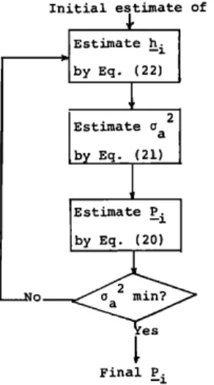
Initial estimate of Pi Estimate h i by Eq. (22) 2 Estimate o a ,by Eq. (21) Estimate P. by Eq. (20) , No- a Final P.
FIG. 1. An algorithm for two-sided AR parameter estimation.
to obtain the following 2n simultaneous equations:
I D(O)
D!I) .
LD( n q- 1) --. D( -- 1)D( -- 2)-'-D( -- n q- 1) D(0) D(--1) D(--nq-2) D(O) (24)di-j di-j+n+
1
]
ßD(
i,
j) = D(
i --j) = di • n-
I
In practice, we do not have the exact values of the covariance
function available, but, instead, we are only given a finite
segment of a time series x(t). So the estimates have to be
obtained from a finite number of data. One method of ob-
taining unbiased estimates of the correlation values is to de-
fine estimators, 1
?(i)
=•
N it,•+
1x(t)x(t--
i).
(25)
There are, of course, a number of different ways of estimat-
ing the autocorrelation sequence from a time series x (t). For
example,
see
Jenkins
and Watts.
12
The parameter estimation procedure relies on Eqs.
(22), (23), and (24) to minimize the value of •. The algo-
rithm is an iterative procedure in which we begin with some
initial estimate
of •i, obtained
from Eq. (22) by dropping
the second term of the right-hand member in (22), acquire the corresponding impulse response function by using Eq.(24), and estimate the residual power by using Eq. (23). This completes one iteration, and by applying (22) again, a
new estimate
of the/•i's is obtained.
This algorithm
is illus-
trated in Fig. 1.The block Toeplitz equations shown in Eqs. (22) and
(24) may be solved by ordinary matrix solution methods,
such as Gauss elimination. These methods require computa- tional time of O(r/3), where n is the number of unknowns. However, due to the special rearrangement of the unknowns, the resulting equations have a regularity that may be exploit- ed in order to reduce the number of computations by an
order
of magnitude.
The block-Levinson•3
algorithm,
which
has a computational
complexity
of O(n2), is presented
in
Appendix A, and may be used for that purpose.III. CONSTRAINED TWO-SIDED AR MODEL
In this section, we constrain the two-sided AR model to
have identical parameters in the forward and backward di-
rections. The model will now be
x(') -- d•x(t -- • ) + d2x (t 9) + ... + d X(t -- n) +d•x(t+ 1) +d2x(t+ 2)
q- '" q- dnx(t q- n) q- a(t). (26) The assumption that the forward and backward param- eters are identical implies that the process is stationary. That
is,
r(i) -- r( - i)
and the symmetric impulse response function hi -- h_ i. Let us multiply both sides of (26) by x(t--i) for i = 1,2,...,n and take expectations. The first equation gives the noise variance in terms of the parameters of the model and the covariances of the process as
rr2• = r(O) -- 2d•r(1) -- 2d2r(2) ... 2dnr(n). (27)
The next n equations may be written in matrix form as
I r(O) r(1)".r(n--1) dl
r(2) r(3)'"r(nq-1)
d•
r'(1)
r(1)
r(0)
r(n
--
2) d2 r(3)
r(4)
'r(n
+
2) d2 r'(2)
Lr(n-
1)
ß r(•) •n r(n
q-
1) ' r(2n)Jn r'(n)
where r'(i) = r(i) - hi•. Also, from Eq. (24), we obtain
1 d• '"dn-1
d• 1 '"dn_ 2 dn 1 ... 1hi
d2 d3...dn+•
h2 d3 d4'..dn+ 2dn+• ... d2n
hl d•h2 =
d2
(28) (29)where
dl/+;I = 0 for li +Jl > n.
It should be noted that the same equations arise when we multiply both sides of Eq. (26) by x(t--i) for i--0,1,...,n and take expectations, due to the stationarity relation and the symmetric impulse response function.
The system of equations in (28) and (29) involves the sum of a Toeplitz plus a Hankel matrix. It was shown in Ref. 14 that this type of equation may be transformed to a block Toeplitz form, and a fast solution can be obtained (see Ap- pendix B). 4. -4 -6
-e
I
Fl=.4^1=,/56
F2=.426^e=•
I I I I II 0 200 400 600 800 ZOO0. TZHE 40. '• 30. •' 20. I-- tO, 0 03 0,0 ' : (b)' TXdI-I-SI]•E]• AR NETHn]• I F1=.402 ' II F2-•423 12TH-BR]]ER ESTIMATE - . w -lO N -J -P0 r-1-30Z -•-••"-
-40 i!
0,00 0,20 0,40 0,60 0,80 1,00 NrlRMALIZEB FREQUENCY (Hz) 40. 30,20,
10,
0,0
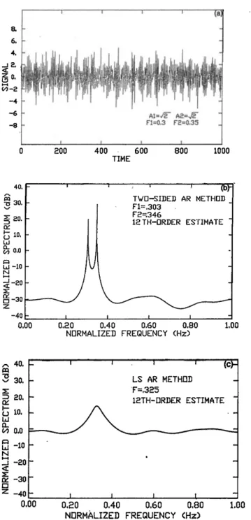
-10 -20 -30 -40 _ o,od - • LS AR METHrlI) - • F:,402 : ! ! iI I ... 0,20 0,40 0,60 0,80 NFIRMALIZEI] FREQUENCY (Hz) 1,00FIG. 2. Spectral estimates of the time series x(n) =
X cos(0.426 rrn) + a(n), in which [a(n) ] isa white Gaussian random pro- cess with variance one. (a) The time series, and spectral estimates obtained' by using (b) the two-sided AR method and (c) the least-squares AR meth-
od.
IV. NUMERICAL EXAMPLES
The constrained two-sided AR model was implemented in order to test the effectiveness of the proposed method. In the simulated case, we try to resolve two closely spaced sinu- soids in the presence of white noise. Specifically, we investi- gate the time series generated by
x(n) =A: cos(rrf•n +•:) + A2 cos(rrf2n +•2) +a(n)
for 1 <n<N, (30)
where •1 --- •2 --- 0, a (n) is a white Gaussian sequence with variance one, and the sinusoidal frequencies are normalized so that f= 1 corresponds to the Nyquist rate. The individual sinusoidal signal-to-noise ratios (SNRs) for this time series
are given
by 20 log
(A •/x/•) for k = 1,2,
where
use
of the fact
that the noise a(n) has variance one has been made. Two
cases will be considered in order to test the performance of the proposed spectral estimator in different noise environ-
ments. These cases have been examined in Refs. 5 and 15,
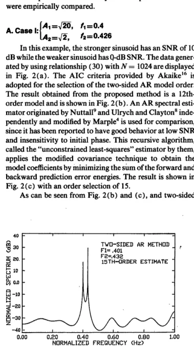
where the performances of many modern spectral estimators were empirically compared.
A.
Case
h
{•11:
A2=x/•,
q•-•,
6:0.4
f2=0.426
In this example, the stronger sinusoid has an SNR of 10 dB while the weaker sinusoid has 0-dB SNR. The data gener- ated by using relationship (30) with N -- 1024 are displayed
in Fig. 2(a). The AIC criteria provided
by Akaike
16 is
adopted
for the selection
of the two-sided
AR model
order.
The result obtained from the proposed method is a 12th- order model and is shown in Fig. 2 (b). An AR spectral esti-mator
originated
by Nuttall
9 and Ulrych and Clayton
8 inde-
pendently
and modified
by Marple
4 is used
for comparison,
since it has been reported to have good behavior at low SNR and insensitivity to initial phase. This recursive algorithm, called the "unconstrained least-squares" estimator by them,applies
the modified
covariance
technique
to obtain
the
model coefficients by minimizing the sum of the forward and backward prediction error energies. The result is shown in Fig. 2 (c) with an order selection of 15.
As can be seen from Fig. 2 (b) and (c), and two-sided
40 - -o 30 - v :>2. ::'0, - I--- 10 • o,o --J -20 [:3 -30 z -40 0,00 i | i ' ' I i --'- ' -- T•D-$II]EI] AR METHDI] FI: .401 F2:.432 15TH---DR]]ER ESTIH•TE ' - - . 0,20 0,40 0,60 0,80 1,00 NDRMALIZEI] FREQUENCY (Hz>
FIG. 3. Two-sided AR spectral estimate obtained using the first 128 data points of case I.
AR spectral
estimator
pro•vides
excellent
•results,
with two
sharp peaks occurring at f, = 0.402 and f2 = 0.423, 'while the AR estimator is unable to resolve the two frequencies in the low SNR environment.
To further demonstrate the ability of the new method, the first 128 points of the data sequence in case I were used to generate a spectral estimate. The resultant 15th-order, two- sided AR spectral estimate obtained is shown in Fig. 3,
where
the ability•to
resolve
the two closely
spaced
sinusoids
(•, = 0.401
and
f2 = 0.432)
is again
evident.
i i I I (a G, 4.
;"
t
:••
,11,
,' r'Jl
-4.-8 I
•
t F1
03
F
I 035
0 200 400 600 BOO 1000 TIME 40, I-- 10. 0 Ld bJ -IO N _1-80 • -3o -40 0.00 TWD-SII)EI) AR METHDD J _ F2-•346I
1RTH-DRDER
ES'FIMATEJ
_ -- i i i i . - 0.20 0.40 0,60 0,80 1.00 NORMALIZED FREQUENCY (Hz) ^ 40. • 80. • lo. co o.o ld -10 - • -80 o• -30 Z -40 ... 0.00 LS AR METHOD F=,325 12TH-DRDER ESTIMATE s J I l 0,80 0.40 0.60 0.80 1.00 NF1RMALIZEI) FREQUENCY (Hz)FIG. 4. Spectral estimates of the time series x(n) = x/• cos(0.3 rrn) +
X cos(0.35 rrn) + a(n), in which [ a( n ) ] is a white Gaussian random pro- cess with variance one. (a) The time series, and spectral estimates obtained by using (b) the two-sided AR method and (c) the least-squares AR meth-
od.
B.
Case
II:
{A•=•/•,
A2=•,
6=0.3
f2=0.35
In this example, the ability to detect more widely sepa- rated sinusoids in a low SNR environment (i.e., 0 dB) is examined. The data generated with N = 1024 are displayed in Fig. 4(a). The same behavior is obtained in this case [shown in Fig. 4(b) ], where the resolution of frequencies is also sharper, and good quality frequency estimates
• = 0.303
andS2
= 0.346
are
obtained
in this
low
SNR
envi-
ronment. For the purpose of comparison, an AR spectral
estimator of 12th order generated by using this data is dis-
played in Fig. 4(c). It is apparent that the AR estimator is
unable to resolve the two frequencies under such a low SNR
condition.
v. CONCLUSION
A new autoregressive model called the two-sided AR model based on interpolation (smoothing) rather than pre- diction has been postulated; based on such a model, spectral
estimation has been done. Simulation examples show higher
resolution capability of the proposed method when com- pared with AR spectral estimation. The matrix equations
arising
in the estimation
procedures
proposed
in this paper
exhibit a special structure. The exploitation of these struc- tures leads to fast solutions that reduce the total number of
computations
by an order of magnitude
compared
with
straightforward approaches.ACKNOWLEDGMENT
The author would like to express his sincere thanks to the anonymous reviewers for their significant suggestions
and comments.
APPENDIX A: FAST SOLUTION OF TWO-SIDED AR EQUATIONS
In this appendix, all the matrices involved will be of
(2 X 2) dimension, whereas the vectors will be of length 2. Algorithm: .
1 •]p,
= R
_•(O)_r•,
(1) xo=Yo
= 0
-
=
(2) For i = 1,2,...,n -- l, do the following:
i--I i
(a) E•, = • R(i--j)x•, E•, = • R(i--j)y,_•,
j=O j=l i--I
(b) _e= • R(i--j)•+,,
j=O(c) B,, = V•-'E,,, By = V ff 'Ey,
Xo Xo 0 Xl Xl Yi- •(d)
i • ' -- ' B,,,
Xi I Yli
•
YO
Yi O_ x
o
Yi-• i • x•
L 1 Xi
1
Yo Yo
[/rx•--[/rx -- gyBx, [/ry•--[/ry -- gxBy ,
(e) g = VZ •[_r'(i)
- _e], where
_r'(i)
= _r(i)
- hi•a,
P-2 P_2 •
(f) ß •_ + g.
/•-i
L y•
!i+ 1 Yo
(3) The solution vector is given by
(elSeL...,eS)
= (a, a
a,_
a _ _,, ... a_, ).
APPENDIX B: FAST SOLUTION OF CONSTRAINED TWO-SIDED AR EQUATIONS
1. Introduction of new notation Let A be an (n) X (n) matrix, A = [a_( 1),a_ (2),...,a_ (n) ]
and
b r= [b(1),b(2),...,b(n) ] = b r(1,n). We define the (n) X (n) operator matrix J= [_e(n)_e(n - 1) ... _e(1)],
where _e(i) is an n X 1 vector with 1 at the ith position and zeros everywhere else, for i = 1,2,...,n. In other words, J has l's along the cross diagonal, and zeros everywhere else. The J matrix performs a reversal operation, such that
AJ r = [q(n),...,q(2),q(1) ],
Jb r= [b(n),...,b(2),b( 1 ) ] = b r(n,1).
The effect of postmultiplication of a matrix by J is thus to reverse the order of the columns. Premultiplications of a matrix A by J reverses the order of the rows of A. Notice, also, that JJ = I, the identity matrix.
Also define a (2n) X (2n) "interleaving" operator Q
such that
! for
i =
2r,
j =
r,
r
- o,
1,...,n
- 1,
{Q}ij =
for i = 2r + 1,j = n + r, r = 0,1,...,n
-- 1,
for all other i, j pairs.
The effect of Q operating on a (2n) x 1 vector is to inter- leave the sequence in the following way'
Q [b(1),b(2),...,b(n),c(1),c(2) .... ,c(n) ]
= [b(1),c(1),b(2),c(2) .... ,b(n),c(n) ].
2. Conversion of Eq. (28) to block Toeplitz form
Let us rewrite the system of equations in Eq. (28) as
Td(1,n) + Hd(1,n) = _r'(1,n), (B1)
where T is an (n)X(n) Toeplitz matrix such that
{T}i• = r(i--j) for i,j = 1,n
and
His an (n) X (n) Hankel
matrix
such
that
{H}ij = r(i + j) for i, j = 1,n.
We may write (B 1 ) in two different ways'
T d(1,n ) + HJJ d(1,n ) = _r' (1,n ), (B2) JTJJ d(1,n) + JH d(1,n) = Jr'(1,n). (B3)
Since T is persymmetric (symmetric around the main
cross diagonal), it can be shown that
and we may rewrite (B2) and (B3) as
T HT•
[•(1,n)]
[•'
1,n
JH
= (n,1)
= _' n,1 '
(B4)
Define $ = HJ and notice that $ is Toeplitz. Since a
Hankel matrix is symmetric, that is, H r =H and
S r = (H J) r = jr H = JH, we therefore conclude that the
coefficient matrix in (B4) consists of four Toeplitz matrices. We now apply the interleaving operation on (B4)
d(1,n)
=Q 3'
(B5)
Q
QrQ
3(n,1) _ (n,1)
and we may group (B5) in terms of (2) X (2) matrices: R(0) R(1) R(n-- 1) -" r'(1)
= r'(2)
r' ('n)
R( -- l)---R( -- n + 1) ]2_1 R(0) '" • t72ß
'n
ß .- R(0) ( ) wherer(i) r(n
+ 1
--
i)
]
R(i)= r(n+l--i)
r(i)
, i--O,n--1,
p_r= [d(i)d(n - i) ], i- 1,n,
_r r = [r(i)r(n - i) ], i = 1,n.
What we have done is to transform an ( n ) X (n) system of equations that involves the sum of a Toeplitz plus a Han-
kel matrix to a (2n) X (2n) system of equations that has a
block Toeplitz form. This will allow us to use the fast block Levinson algorithm to solve the equations efficiently.
I A. Papoulis, "Maximum entropy and spectral estimation: A review," IEEE Trans. Acoust. Speech Signal Process. 29(6), 1176-1186 (1981 ). 2j. Makhoul, "Linear prediction: A tutorial review," Proc. IEEE 63, 561-
580 (1975).
3S. M. Kay and S. L. Marpie, "Spectrum analysis--A modern perspec- tive," Proc. IEEE 69, 1380-1419 ( 1981 ).
4L. Marpie, "A new autoregressive spectrum analysis algorithm," IEEE Trans. Acoust. Speech Signal Process. 28(4), 441-453 (1980). 5j. A. Cadzow, "High performance spectral estimation--A new ARMA
method," IEEE Trans. Acoust. Speech Signal Process. 28(5), 524-529
(1980).
6j. Makhoul, "Stable and efficient lattice methods for linear prediction," IEEE Trans. Acoust. Speech Signal Process. 25(5), 423-428 (1977). 7p. R. Gutowski, E. A. Robinson, and S. Treitel, "Spectral estimation, fact
or fiction," IEEE Trans. Geosci. Electron. 16(2), 80-84 (1978). ST. J. Ulrych and R. W. Clayton, "Time series modelling and maximum
entropy," Phys. Earth Planet. Inter. 12, 188-200 (1976).
9A. H. Nuttall, "Spectral analysis of a univariate process with bad data points, via maximum entropy and linear predictive techniques," Naval
Underwater Systems Center, New London Laboratory, NUSC Tech. Rep.
5303 (26 March 1976).
•oy. A. Rozanov, Stationary Random Process (Holden-Day, San Francisco, 1967), Chap. 1, pp. 1-50.
•G. E. Box and G. M. Jenkins, Time Series •4nalysis, Forecasting and Con- trol (Holden-Day, San Francisco, 1976).
•2G. M. Jenkins and D. G. Watts, Spectral •4nalysis and Its •4pplications (Holden-Day, San Francisco, 1968).
•3H. Akaike, "Block Toeplitz matrix inversion," SIAM J. Appl. Math. 24,
234-241 (1973).
•4A. M. Gulamabbas and T. W. Parks, "Efficient solution of a Toeplitz- plus-Hankel coefficient matrix system of equations," IEEE Trans. Acoust. Speech Signal Process. 30( 1 ), 40 •. (1982).
•ST. M. Sullivan, P. L. Frost, and J. R. Treichler, "High resolution signal estimation," ARGO Systems, Inc., Tech. Rep. (June 1978).
•6A. Akaike, "Statistical predictor identification," Ann. Inst. Stat. Math.