New nonlinear algorithms for estimating and suppressing narrowband interference in DS spread spectrum systems

ew Nonlinear Algorithms for Estimating

uppressing Narrowband Interference

in

DS

Spread

Spectrum

Systems

Wen-Rong Wu,

Member,

Abstract-It has been shown that the narrow-band (NB) inter- ference suppression capability of a direct-sequence @S) spread spectrum system can be enhanced considerably by processing the received signal via a prediction error filter. The conventional approach to this problem makes use of a linear filter. However, the binary DS signal, that acts as noise in the prediction process, is highly non-Gaussian. Thus, linear filtering is not optimal. Vijayan and Poor [ll] first proposed using a nonlinear approx- imate conditional mean (ACM) filter of the Masreliez type and obtained significant results. This paper proposes a number of new nonlinear algorithms. Our work consists of three parts. 1) We develop a decision-directed Kalman (DDK) filter, that has the same performance as the ACM filter but a simpler structure. 2) Using the nonlinear function in the ACM and the DDK filters, we develop other nonlinear least mean square (LMS) filters with improved performance. 3) We further use the nonlinear functions to develop nonlinear recursive least squares (RLS) filters that can be used independently as predictors or as interference identifiers so that the ACM or the DDK filter can be applied. Simulations show that our nonlinear algorithms outperform conventiond ones.

I. INTRODUCTION

PREAD-SPECTRUM techniques provide an effective way to cope with narrow-band (NB) interference in communi- cation systems [l]. The basic idea behind these techniques is to spread the bandwidths of transmitting signals so that they are much greater than the information rate. In a direct se- quence (DS) spread spectrum system, bandwidth spreading is realized by modulating the transmitting signal with a pseudo- noise (PN) signal. At the receiver, the signal is de-spread by correlating it with the same PN sequence. This system can reject interference whose bandwidth is small compared to the spread signal. It has been shown [2]-[ 111 that the capability of the DS spread spectrum systems to reject NB interference can be further improved by processing the received signal. This is because there exists strong correlation in the

N B

signals. Thus, the interference can be predicted from its past values. However, the spread signal is white and cannot be Paper approved by J. S. Lehnert. the Editor for Modulation and Signal Design of the IEEE Communications Society. Manuscript received May 10, 1994; revised March 28, 1995 and August 21, 1995. This paper was presented in part at the 1995 International Symposium on Communications, Taipei, Taiwan, December 27-29, 1995. This work was supported by the National Science Council, Taiwan, ROC 83-0404-E-009-105.

W.-R. Wu is with the Department of Communication Engineering, National Chiao Tung University, Hsinchu, Taiwan, ROC.

F.-F. Yu is with Chroma Inc., Taipei, Taiwan, ROC. Publisher Item Identifier S 0090-6778(96)03 142-X.

[EEE, and

Fu-Fuang Yu

predicted. Once the prediction of the interference is obtained, an error signal is computed by subtracting the estimate from the received signal. This error signal is then used as the input of the correlator.

In [2]-[5], Hsu and Giodano, Keltchum and Proalus, Iltis

and Milstein applied linear transversal filters to the problem of

NB interference rejection. Masry gave closed-form expressions for the signal-to-noise ratio (SNR) improvement [6], [7]. Linear least mean square (LMS) estimation techniques offer an adaptive way of prediction. One distinct advantage of the LMS algorithm is its simplicity. Li and Milstein [SI applied the algorithm to the NB interference rejection problem. Iltis and Milstein then analyzed the performance in [9]. Though the linear filtering approach has yielded fruitful results, one problem has been overlooked. In the prediction of interfer- ence, the DS signal acts as noise. Since noise degrades the performance of the LMS algorithm, direct use of the algorithm cannot produce optimal results. To remedy this problem, we can filter the received signal before it enters the transversal filter. This approach will be elaborated in this paper.

Another approach is to obtain the state-space representa- tion of the system so the well-known Kalman filter can be applied. Since the DS sequence, which can be modeled as an independent, identically distributed (i.i.d.) binary sequence, is non-Gaussian, the Kalman filter is not optimal. The optimal filter in this case is nonlinear. To solve this problem, Vijayan and Poor Ell] modeled the

NB

interference as an AR process and applied a Masreliez-type approximate conditional mean (ACM) filter. The performance of this approach is significantly better than the Kalman filter. However, the problem with this approach is the difficulty of identifying the AR parameters. Since the poles of the AR model are close to the unit circle, standard recursive identification schemes cannot work satisfactorily. Therefore, Vijayan and Poor used the nonlinear function in the ACM filter to develop adaptive nonlinear LMS type of algorithms that do not need the system model. They showed that nonlinear LMS algorithms perform appreciably better than linear ones. These algorithms were extended by Rusch and Poor [12] to suppress

NB

interfercncc in CDMA spread spectrum systems.

In this paper, we propose new nonlinear algorithms to suppress

NB

interference. Our contribution has three parts. First, to simplify the computational complexity of the non- linear functions in the ACM filter, we propose a decision- directed Kalman (DDK) filter. While the DDK filter retains the 0090-6778/96$05.00 0 1996 IEEE

WU AND YU: NEW NONLINEAR ALGORITHMS FOR ESTIMATING AND SUPPRESSING NARROWBAND INTERFERENCE

~

509

performance of the ACM filtering, it requires less computation. Second, we develop nonlinear LMS types of algorithms by employing estimation theory. As mentioned above, the input to the LMS algorithm is contaminated by non-Gaussian noise. Better results can be obtained by filtering the noisy input. Since the noise is non-Gaussian, the LMS algorithm becomes nonlinear. This concept of “input filtering” can be applied to the recursive least squares (RLS) algorithm, resulting in nonlinear RLS algorithms. This leads to the third part of our work. We propose to employ the nonlinear RLS algorithm to identify the AR parameters of interference and then apply the ACM or the DDK algorithm to perform filtering in the state space domain. We show that nonlinear I U S algorithms perform well even when the poles of the AR model are close to the unit circle.

The organization of this paper is as follows. Section 11 provides a brief review of the LMS algorithm and related nonlinear algorithms in [ l l ] and [12]. In Section 111, new nonlinear filters are derived. Simulations are described in Section IV. Section V presents our concluding remarks.

IT.

LMS AND ACM FILTERING

A. System Model

We follow the model described in [ I l l . The low-pass equivalent of a DS spread spectrum modulation waveform is given by

N,-1

m ( t ) =

1

C k 4 ( t - k T c ) (1)

k=O

where N , is the number of PN chips per message bit, T~ is the chip interval, C k is the kth chip of the PN sequence, and q ( t ) is a rectangular pulse of duration T ~ . The transmitted signal is expressed as

s ( t ) = b”t

-

kTb)

k

where { b k } is the binary information sequence and Tb =

M,r,

is the bit duration. The received signal is defined by

Z ( t ) = as(t - T )

+

n ( t )

+

i ( t ) (3) where a is an attenuation factor, T is a delay offset, n ( t ) is wideband Gaussian noise, and i ( t ) is narrow-band interference. Here, we assume that n(t) is bandlimited and becomes white after sampling. For simplicity, let T be zero and a = 1. Suppose that the received signal is chip-matched and sampled at the chip rate of the PN sequence. We thus have

z k = s k f nk

+

ik ₍₄₎

where { s k ) , { n k } , and { i k } are the discrete-time sequences

from { s ( t ) } , { n ( t ) } , and { i ( t ) } , respectively. { s k } , { n k } , and { i k } are assumed to be mutually independent. Since the PN sequence is random, we can consider { S A } to be a sequence of i.i.d. random variables taking values of

+

1 or - 1 with equal probability.

B. LMS Algorithm

Let the tap weights of a transversal filter be (al,

. .

.

,

ah}. The tap-weight update equations of the LMS algorithm can be expressed as

01, = ek-1

+

/ / k k X k ( 5 )

where Ok = [ u l , k u 2 , k

..

.

UL,~]‘ is the estimated tap weight at time k ,

Xk

= [ z k - l Z k - 2

...

Z I , - L ] ~ is the

input vector, and c k = z k - X f 0 k - l is the prediction

error. For the suppression of NB interference, it has been shown that better results can be obtained by using a two- sided LMS filter. For this filter, 0 k and X I , are changed

X k = [ z ~ + N Z ~ + N - I z1,+1 z k - 1

‘ . .

X L - N ] . To make

the step size invariant with respect to the input power, a normalized LMS algorithm is frequently used. This algorithm is defined as (6) A A a to 01, = [ U - i v , k U - N + I , ~ ‘0. a - l , k ~ 1 , k

. . .

U N , ~ ] ~ and A P @ k + l = 01,

+

- E k X k r k

where Tk is an estimate of the input power, that can be obtained by

r k = p r k - l + (1 - P)Z~. (7) ,@, 0

<

p

<

I, is a forgetting factor chosen to yield a compromise between the prediction accuracy and the tracking capability.

C. Approximate Conditional Mean (ACM) Filter

process of order p , i.e.,

Assume that the NB interference { i k } is a Gaussian AR P

i k = 4 3 i k - 3

+

dk (8)

3=l

where the AR parameters (41, .

.

.

,

&} are known to the re- ceiver and (&} is a white Gaussian process of zero mean and variance a:, i.e., pek

(x)

N Nup (x), where

Nu2(x)

= 1 / 6 0

exp{-x2/2a2}. From (8), we can construct a state space representation for the received signal and the interference

XI, = @ X k - l f W k (9) X k = H X k $. Vk (10) where X k = [ i k i k - 1

. . .

i k - p + l ] T , wk = [ d k 0

. . .

O I T ,

N

=

[I

0 . * . 01, ~k = s k

+

n k , and 0 0 1 0 $ l , k 4 2 , k ” ’ + p - l , k & , k

:

1.

(11) c p = 1 0 1 1 0

. . .

. . .

...

. . . ...

...

. . .

0 0

. . .

The estimate of X k based on observations until time k is referred to as the filtering problem, and the estimate of X I ,

based on observations until time k - 1 is referred to as the prediction problem. It is known that the optimums of such estimates, in the minimum mean square error sense, are

E{XklZ"'}, where Z k = (21 2 2

. . .

~ k } . When {wk} be recursively obtained from the well-known Kdman filter. However, uk is the sum of two independent random variables; one is Gaussian distributed and the other takes on values f l or -1 with equal probability, Le.,

aIgorithm is described as follows:

(21)

and {wk} are Gaussian processes, the optimal estimates can _{P A}

O k = Ok-1

+

- E k X k rli where

T O k [ Q , k U 2 , k

. . .

U L , k I

Such a sequence is highly non-Gaussian. The optimal filter z k = C&, R-12k-z

for such a sequence is nonlinear. In [14], Masreliez developed an ACM filter to estimate the state of a linear system with

non-Gaussian observation noise. If we assume that the state = a 2 , k - 1 [ z k - z

+

P ( E k - z ) l . (24)

prediction density p ( X k

1

2

"

'

)

is Gaussian with mean x k and

2=1 L

z=1

E k = Zk - zk, and T k

nodinear function of f k defined by

covariance M A , the conditional mean X k and its covariance

Pk can be recursively calculated as

plrk-l

+ (1 -

p1).,2.

P ( , ) is a

Mk+i

=

@PkaT

+

Q k (15) and can be estimated by

Xk+l = @ x k (16)

-

32 = A, - 1 ₍₂₆₎

where Ak is a sample estimate of the prediction error variance that can be obtained by Ak = P z A k - 1

+

(1 - @,)E;.

p1

and S k ( Z k ) = [y(~klZ"-')]-l (17)

,&

are forgetting factors with values between zero and one. In

[12], Rusch and Poor modified (21) into where

[

zli (27) P T k Ok = O k - l

+

-

P ( € k ) X k (18) and Qlc = E{wkwZ}. The function g ( . ) is called the score

function. Vijayan and Poor employed this algorithm to solve the NB interference suppression problem in the DS spread spectrum system [ 113. By the model in (9) and (lo), the score function and its derivative turn out to be

% k ( Z k )

G k ( Z k ) = ___

showing that (27) can provide better results.

III.

NEW NONLINEAR ALGORITHMS

A. Decision-Directed Kalman (DDK) Filter

From the last section, we know that the performance of the ACM filter will be nearly optimal. The computation of the score function and its derivative, (19) and (20), however,

(

H M ~ H T

+

$)]

(19) involves the W(.) and sech (.) functions which are not efficient. To improve the computational efficiency, we now propose a DDK filter. The density of the observation noise is a Gaussian mixture, ;.e.,

1 HMk HT

+

g: g k ( Z k ) Zk - Hzk 1 HA4kHT

+

0: 1 ( W M k H T

+

0:) and - G k ( Z k ) =

P ( v ~ ) =

;[No?

(uk -

1)

+

No;

(nk 4 I)]. (28)

(20)

We can construct hypotheses equivalent to (28) as follows:

It can be seen that the ACM filter has a structure similar to that of the standard Kalman filter. The time update equations (15) and (16) are identical to those in the Kalman filter. The measurement update in (13) involves the correction of the predicted value by a nonlinear score function. The nature of the nonlinearity is determined by the density function of the

P ( ~ o ) = p ( ~ l ) ~ 0.5. Given H~ or H ~ , the optimal state

estimator is just the ~~l~~ filter, Let

observation noise. P ( Z k

Izk-I)

= N M k ( Z k - :k) (31)

where 51, is the mean of p ( z k l 2 " ' ) . We then have

D. Adaptive Nonlinear LMS Prediction Filter

Vijayan and Poor also developed an adaptive nonlinear LMS 2 k = Zk

+

M k H t ( H M k H t

+

d1-l

(2k - Hzk - 1) (32)

WU AND Y U NEW NONLINEAR ALGORITHMS FOR ESTIMATING AND SUPPRESSING NARROWBAND INTERFERENCE

~

511

if

HO

is given and

if H I is given. Note that the error covariance matrix is the

same in both cases. If we can determine which hypothesis is true, we can apply the corresponding Kalman filter. This is the standard hypotheses testing problem. Thus, we have to evaluate

~ ( H ~ I z ~ )

where i = 0 or 1. Since p ( H 0 ) = p(H1) = 0.5 and

p ( z k l ~ k - 1 ) is a constant, P(H;JZ') is proportional to p(zklzk, Hi). It is simple to show that

Thus, the optimal decision rule is

Observing (37) and (38), we find the decision is simple to carry out, i.e.,

If z k

-

HBk

2

0 , Choose Ho. (41) If z k - HTk

<

0, Choose HI. (42) Summarizing the results developed above, we have obtained the DDK filter described as follows:

xk

= X k

+

M ~ H ~ ( H M ~ H ~

+

.

[ z k - H x k - sgn ( z k - H;i?k)] Xk+l =@X.k (45) Mk+i = @PkaT

+

Q k (43) Pk = Mk

-

A!ikHT(HA!ikHT

+

a;)-'HA!ik (44) - (46) where

Except for (43), the other equations are the same as the standard Kalman equations. The measurement update in (43) is a nonlinear function of %k - H x k . The nonlinearity is determined only by the sign of the prediction error. The com- putational complexity is then greatly reduced. It is interesting to consider the sgn(.) function as an approximation of the tanh(.) function. From the simulation results in Section IV, we find that the performance of the DDK filter is almost the same as that of the ACM filter.

B. Nonlinear Adaptive LMS Filters

The performance of the LMS algorithm will be degraded if noise is present. For the NB interference suppression problem, the only information we have is the noisy observation Zk. The

noise consists of the binary DS signal and Gaussian noise. Most previous work ignored this fact and directly used Zk

as the desired signal. In 1111, Vijayan and Poor first pointed out this problem and used a nonlinear processing strategy. However, it is not clear how their algorithm is derived and what it means. Here, we approach this problem with the concept of input filtering and use estimation theory to solve it. Given the observations

Z k ,

we assume that p ( i k ( 2 " ' ) N

Nu;(ik - pk). Without knowledge of the AR coefficients, computation of b k and 0; is difficult. For the time being, let us assume that at time k - 1, the tap-weight vector Ok-l represents the true AR coefficients, then, from (S), we have

pk = E{iklZ"-l}

= E { [ i k - I , i k - 2 ,

* " ,

ik-L,]Ok-1+dklZk-l}

= [E{ik-112"'},

.

* .

,

E{ik-LJZ"-l}]O&l. (47) Since i k is an NB signal, it is then reasonable to make the following approximation:

[ E { i k - ' I z k - 1 } ,

. . . ,

E{ik&iJZ"-l}]

M [E{i&1IZ"-l},

. . .

,

E{il,-LJZ"-L}] = [ i k - l , i k - 2 ,

- . .

,

i k 4 ]

=

x;.

₍₄₈₎

From (47) and (48), we find that if X k is available at time k

and is used as the i\put to the LMS predictor, the output of the predictor i k = XrOk-1 will be &. We can also show that the prediction error variance 0: will be 0;. We then have (49) A

P(iklZ"1) N & ( i k -

Q.

From (4), we have

Zk = i k

+

'Uk and U k = ??,1;

+

S k . (50)

The prediction error is then

where f ? k is the prediction error in the absence of the non- Gaussian noise vk, i.e.,

p ( e k ~ ~ " - l ) = N u g ( e k ) . (51) Note that e k is independent of 'Uk. Thus, the prediction error signal ~k used in the LMS contains the noise v k , that will

degrade the performance. We can remedy this problem by filtering Q. From the Baye's law, we have

estimate

&

from E , based on observations until time k is

the approximate conditional mean. One can show that f?k =E{ekJZk}

-

-

.

,

"

[ E k - tanh

.

(&)I

(53)

0,"

+

0:

We can also use the decision-duected algorithm and obtain the estimate

[a

- sgn ( E k ) ] .

e k = ___

4

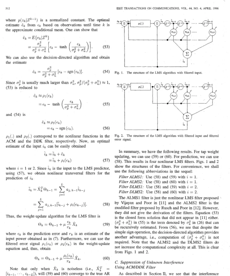
_{(54) Fig. 1. The structure of the LMS algorithm with filtered input.}

g;

+

fl:

Since a; is usually much larger than a:, o,"/(o,"

+

0:) M 1,

( 5 3 ) is reduced to

and (54) is

e k " P Z ( E k )

= € k - sgn(€k). (56)

P I ( . ) and p 2 ( . ) correspond to the nonlinear functions in the

ACM and the DDK filter, respectively. Now, an optimal estimate of the input ik can be easily obtained

A

-ik = ik

+

' i k

+

P % ( E k ) (57)

where i = 1 or 2. Since z k is the input to the LMS predictor,

using (57), we obtain nonlinear transversal filters for the prediction of i k

j=1

L

= aJ,k--1[2k--3

+

P&k--3)1. ( 5 8 )

3=1

Thus, the weight-update algorithm for the LMS filter is (59)

Ek T k Ok = p,

-

x,

where E , is the prediction error and T k is an estimate of the

input power obtained as in (7). Furthermore, we can use the filtered error signal p l ( t k ) or , o z ( E ~ ) in the weight-update equation and, thus, obtain

Note that only when X k is noiseless (i.e., Xr = [ i k - l ,

. . .

,

z k - ~ ] ) , will (59) and (60) converge to the true AR coefficients. On the other hand, only when Ok-1 represents the

true AR coefficients, will

a,

in ( 5 8 ) be p k . When k is small,

these assumptions are not true. Through the two-step iteration scheme; ineut-filtering and weight-updating, however, as 5 increases, X , will become less and less noisy and 01, will approach the true AR coefficients.

Fig. 2. The structure of the LMS algonthm with filtered input and filtered error signal.

In

summary, we have the following results. For tap weight updating, we can use (59) or (60). For prediction, we can use (58). This results in four nonlinear LMS filters. Figs. 1 and 2 show the structures of the filters. For convenience, we shall use the following abbreviations in the sequel:

FiZterALMSl: Use ( 5 8 ) and (59) with i = 1. FiZterALMS2: Use ( 5 8 ) and (60) with i = 1.

Filter DLMSI: Use ( 5 8 ) and (59) with i = 2.

Filter DLMs2: Use ( 5 8 ) and (60) with z = 2.

The ALMS1 filter is just the nonlinear LMS filter proposed \

by Vijayan and Poor in [Ill and the ALMS2 filter is the modified filter proposed by Rusch and Poor in [12]. However, they did not give the derivation of the filters. Equation (53) is the closed form solution that did not appear in [ 111 either. (0;

+

0:) in (55) is the term denoted by a: in (26) that can be recursively estimated. From (56), we see that despite the simple sign operation, the decision-directed algorithm provides another advantage, i.e., computation of (0,"

+

0:) is not required. Note that the ALMS2 and the DLMS2 filters do not increase the computational complexity at all. This is clear from Figs. 1 and 2.

C. Suppression of Unknown Intetjierence Using ACMDDK Filter

As described in Section 11, we see that the interference and the received signal can be formulated in a state space representation and the ACM or the DDK filter can be applied. However, the AR parameters of interference have to be known. In real applications, we cannot determine the parameters in advance. One possible solution is to perform parameter estimation first and then apply the ACM or DDK filter.

WU AND YU: NEW NONLINEAR ALGORITHMS FOR ESTIMATING AND SUPPRESSING NARROWBAND INTERFERENCE 513

Vijayan and Poor mentioned this method in [ll]. Since the poles of the AR model are close to the unit circle, standard recursive identification schemes such as recursive maximum likelihood (RML) algorithm [ 151-[ 171 converge rather slowly. In addition, the performance of the ACM filter is sensitive to parameter variation. Consequently, this method was not successfully implemented in [ 111. Here, we propose to use the RLS method to identify the AR parameters. It is well- known that the RLS algorithm converges faster than the LMS algorithm. However, when the observations contain noise, the performance of the standard I U S algorithm is seriously degraded. We shall use the concept of “input filtering” to combat this problem. Because the filtering mechanism is similar to that of the LMS algorithm, the results developed above are directly applicable here. The standard RLS algorithm is given as

E k = Zk - OT k - l x k

PI, =A-‘Pk-l

-

A-‘KkX,TPk-l (64) (62)

01, = O I , - ~ + K k ~ k (63)

where 01, is the tap weight vector of the filter, X is the forgetting factor, and

xk

= [ ~ k - l

...

zk-LlT is the input. Thus, X I , can be replaced by its filtered version XI, as defined in (48) and (57). The error signal E k in (63) can also be replaced by p ; ( ~ k ) . Then, we have the four nonlinear RLS algorithms described below

Ck = Z k - @ z - l x k (66)

Ok = @ & I

+

K k f ( € k ) (67) Pk = A - l P k - 1

-

A - l K k X , T P k - l . (68) FilterARLSl: Use P I ( . ) in X k and ~ ( E I , ) = ~ k .

Filter ARLS2: Use p~ (.) in

XI.

and f ( ~ k ) = p 1 ( ~ g ) . Filter DRLSl: Use p2(.) in Xk and f ( ~ ) = ~ k . Filter DRLS2: Use p2(.) in X k and f ( ~ ) = p2(~k). ARLS2 and DRLS2 will be selected to perform the identifi- cation since they have better performance. It will be shown that both algorithms can adapt quickly to an unknown environment. For convenience, in the simulations reported below, we refer to the scheme with the ARLS2 algorithm and ACM filter as AR2A and the scheme with the DRLS2 algorithm and DDK filter as DR2D.

IV. SIMULATIONS

In this section, we report on simulations carried out to evaluate the performance of the proposed algorithms. We follow the examples studied in [ll]. We first define our performance measure, which is the commonly used SNR improvement. We define this as follows:

Output SNR

2

lolog

[

E(,E:(!:k,2)] dB (70)

where ~ k : is the prediction error. Therefore

The SNR at the input was varied by changing the power of the interfering signal. The variance of the background thermal noise was kept constant at uz = 0.01. All results were obtained based on 20 trials, and for each trial, 5000 data points were computed. The number of filter taps was 10. Two kinds of NB interference were considered: AR and sinusoidal interference. We first considered the AR interference. The AR interfering signal was obtained by passing white noise through a second- order IIR filter with two poles at x = 0.99, i.e.,

ik = 1.98ik-1

-

0.98Olik-2

+

d k (72) where { d k } is white Gaussian noise. Four sets of simulations

conducted:

The AR parameters were assumed to be known; three filters were compared, namely, Kalman, ACM, and DDK.

The

AR

parameters were assumed to be unknown; five types of LMS filters were compared, namely, normalized

two-sided LMS (TS-LMS), ALMS1, ALMS2, DLMS1,

and DLMS2.

The AR parameters were assumed to be unknown; five types of RLS filters are compared, namely, RLS, ARIS1, ARLS2, DRLS1, and DRLS2.

The AR parameters were assumed to be unknown; two schemes were compared, namely, AR2A and DR2D. Table I summarizes the results (predictions) of the four sets of simulations. It can be seen that adaptive nonlinear filtering techniques offer considerable advantages over conventional linear filters. The performance of the decision-directed al- gorithms is almost as good as that of ACM. In the known interference case, the linear Kalman filter performs poorly. The ACM and the DDK have the same results. This is due to the precise state prediction, by which the error is very close to f l or -1. In this case, the sign function is almost equal to the tanh(.) function. For LMS filters, we can see that ALMS2DLMS2 perform the best, with an SNR improvement significantly higher than that of the TS-LMS algorithm. The performance of ALMSlDLMSl is between

that of TS-LMS and ALMS2DLMS2. From part three of

Table 1, we find that the standard IUS algorithm is greatly affected by the non-Gaussian DS signal. Its performance is even worse than that of TS-LMS. The reason for this is as follows. The vector Kk in (63) can be viewed as a product of the step size and the input vector. The step size in the LMS algorithm is constant. However, it keeps decreasing in the RLS algorithm. The rate of decrease must be synchronized with the rate of convergence. When X I , is noisy, KI, is not

correctly evaluated and this synchronization is destroyed. This is why the RLS performs poorly in a noisy environment. The influence of ~k is not that crucial, since KI, is small when the filter converges. Thus, the difference in the performance of

Input

SNR

(dB) -20 -15 -10 Kalman 26.73 23.51 20.27 ACM 36.87 32.57 28.10 DDM 36.87 32.57 28.10 -5 16.95 23.50 23.50

SNR IMPROVEMENT FOR AR INTERFERENCE

\ I Kalman ACM DDK I 39.76 34.79 29.80 24.80 39.66 34.89 29.91 24.91 38.44 34.25 29.68 24.74 I I DLMS2 RLS ARLSl I 36.41 32.07 27.50 22.92 24.48 20.90 16.85 12.32 36.31 31.84 27.15 22.41 DRLSl ARLS2 DRLS2 AR2A DR2D

ARLSlDRLSl and ARLSZ/DRLS2 is not significant. Finally, we see that AR2AlDRZD perform satisfactorily. This indicates that ARLS2DRLS2 did identify the interference properly. One point worth noting is that the performances of ACM, DDK,

ALMS2, DLMS2, ARLS2, DRLS2, AR2A, and DR2D are all

very similar, regardless of whether the interference parameters are known. It seems that the performance bound is reached and the state space formulation cannot provide additional improvement.

Another case we considered was that of sinusoidal interfer- ence. The frequency of the sinusoidal interference signal was kept constant at 0.15 radians, i.e.,

(73)

where A is the amplitude and 8 is a random phase with uniform distribution. Table I1 shows the simulation results. From the figure, we see that the performance is similar to that in the AR interference case. One difference is that since the interference in this case is deterministic, the performance of the Kalman filter is not affected by noise (only convergence speed is affected).

On the basis of the simulation results, we conclude that the nonlinear algorithms developed in this paper indeed provide good performance. We particularly recommend the DLMS2 filter, that typically provides the best performance at a com- putational cost as low as that of the LMS filter. For fast convergence, the DRLS2 filter is a good choice; while its convergence speed and performance are equivalent to those

of the ACM filter, it is simpler to implement.

i ( t ) = A COS (0.15t

+

8)

36.28 31.84 27.15 22.41 36.85 32.49 27.86 23.18 36.85 32.49 27.86 23.18 36.99 32.68 28.15 23.44 36.99 32.68 28.15 23.44

SNR IMPROVEMENT FOR SINUSOIDAL INTERFERENCE

_ _ _ ~ DRLS2 AR2A

DR2D

Inout

SNR

(dB)

I

-20

1

-15

I

-10

I

-5

I 38.01 33.24 28.37 23.35 38.52 33.63 28.72 23.77

38.52

33.63 28.72 23.77 , ALMS2 RLS 23.74

I

18.72 ARLSl

I

37.79

1

32.95

-3”

13.83

1

I 9.224 28.08

I

23.09 I I I DRLSl

I

37.66

I

32.86

I

28.01

I

22.96 ARLS2

I

37.97

I

33.21

1

28.43

1

23.47

received signal contains a highly non-Gaussian signal. The input to the predictor is noisy. Better performance can be obtained by properly filtering the input. Since the noise is non-Gaussian, the optimal filter is nonlinear. In this paper, we have proposed nonlinear algorithms, described as follows:

1) We have developed a DDK filter for known interference. The DDK filter is computationally simpler than the previously proposed ACM filter, but provides the same level of performance.

2) We have developed nonlinear LMS filters that result in better performance and less computation.

3 ) We have developed nonlinear RLS algorithms that can be used independently, or as interference identifiers so that the ACM or the DDK filters can be applied. Simulations show that our nonlinear filters perform signif- icantly better than conventional ones. Among the proposed filters, DLMSZ and DlUS2 are the most useful. The proposed DLMS2 filter performs as well as filters formulated in state space, such as the ACM filter, but has a structure as simple as that of an LMS filter. The proposed DRLS2 filter offers fast convergence without involving the system model. It is mentioned in [ 1 11 that the nonlinear function of the ACM filter will become a hard limiter when

0-2

-+ 0. This is different from our scheme. We derive the decision-directed algorithms based on the formulation of hypotheses testing and we do not assume

CT; = 0. In fact,

02

will not be zero. That’s why Vijayan

and Poor used the tanh(.) function as a soft limiter. Finally, our results show that the state space approach cannot provide better results in the NB interference suppression problem. V. CONCLUSIONS

REFERENCES

In this paper, we have considered nonlinear prediction filters for the rejection of NB interference in the DS spread spectrum use of linear LMS filters. However, it is known that the

[I1 G R Cooper and C D McGlllem, Modern Communzcatzon and Spread Spectrum New York, McGraw-Hill, 1986

[2] F M Hsu and A A Giordano, “Digital whitening techniques for im- proving spread-spectrum Lommunications performance in the presence

WU AND YU: NEW NONLINEAR ALGORITHMS FOR ESTIMATING AND SUPPRESSING NARROWBAND INTERFERENCE 515

of narrow-band jamming and interference,” IEEE Trans. Commun., vol. COM-26, pp. 209-216, Feb. 1978.

J. W. Keltchum and J. G . Proakis, “Adaptive algorithms for estimat- ing and suppressing narrow-band interference in PN spread-spectrum systems,” IEEE Truns. Commun., vol. COM-30, pp. 913-924, May 1982.

L. M. Li and L. B. Milstein, “Rejection of narrow-band interference in PN spread-spectrum systems using transversal filters,” IEEE Trans.

Commun., vol. COM-30, pp. 925-928, May 1982.

R. A. Iltis and L. B. Milsten, “Performance analysis of narrow-band interference refection techniques in DS spread-spectrum systems,” IEEE Trans. Commun., vol. COM-32, pp. 1169-1 177, Nov. 1984.

E. Masry, “Closed-form analytical results for the refection of narrow- band interference in PN spread-spectrum systems-Part I: Linear predic- tion filters,” IEEE Trans. Commun., vol. COM-32, pp. 888-896, Aug.

1984.

-, “Closed-form analytical results for the refection of narrow- band interference in PN spread-spectrum systems-Part 11: Linear interpolation filters,” IEEE Trans. Commun., vol. COM-33, pp. 10-19,

Jan. 1985.

L. M. Li and L. B. Milstein, “Rejection of pulsed CW interference in PN spread-spectrum systems using complex adaptive filters,” IEEE Trans. Commun., vol. COM-31, pp. 10-20, Jan. 1983.

R. A. Iltis and L. B. Milstein, “An approximate statistical analysis of the Widrow LMS algorithm with application to narrow-band interference refection,” IEEE Trans. Commun., vol. COM-33, pp. 121-130, Feb.

1985.

E. M a r y and L. B. Milstein, “Performance of DS spread spectrum receiver employing interference suppression filters under a worst-case jamming condition,” IEEE Trans. Commun., vol. COM-34, pp. 13-21,

Jan. 1986.

R. Vijayan and H. V. Poor, “Nonlinear techniques for Interference suppression in spread-spectrum,” IEEE Trans. Commun., vol. 38, pp.

1060-1065, July 1990.

L. A. Rusch and H. V. Poor, “Narrowband interference suppression in CDMA spread spectrum communications,” IEEE Trans. Commun., vol.

42, pp. 1969-1979, Apr. 1994.

S. Heykin, Adaptive Filter Theory. Englewood Cliffs, NJ: Prentice-

Hall, 1991.

[14j C. J. Masreliez, “Approximate non-Gaussian filtering with linear state and observation relations,” IEEE Trans. Automat. Contr., pp. 107-1 10,

Feb. 1975.

[15] L. Lung and T. Soderstom, Theory and Practice of Recursive Identi$- cation. Cambridge, M A MIT Press, 1983.

[ 161 B. Friedlander, “System indentification techniques for adaptive signal processing,” IEEE Trans. Acoust. Speech, Signal Processing, vol. ASSP-

30, pp. 240-246, Apr. 1982.

[17j -, “A recursive maximum likelihood algorithm for ARMA line enhancement,” IEEE Truns. Acoust. Speech, Signal Processing, vol.

ASSP-30, pp. 651-657, Apr. 1982.

Wen-Rong Wu (S’87-M’89) was bom in Taiwan, ROC, in 1958. He received the B.S. degree in mechanical engineering from Tatung Institute of Technology, Taiwan, in 1980, the M.S. degrees in mechanical and electrical engineering, and the Ph.D. degree in electrical engineering from the State University of New York, Buffalo, in 1985, 1986, and 1989, respectively.

Since August 1988, he has been a faculty member in the Department of Communication Engineering in National Chiao Tung University, Taiwan. His research interests include statistical signal processing and digital communi- cations.

Fu-Fuang Yu was bom in Taiwan, ROC, in 1968. He received the M.S. degree in communication engineering from National Chiao Tung University, Taiwan, in 1993.

Currently, he is an Engineer in Chroma Inc. in Taiwan. His research interests include communications and signal processing.