行政院國家科學委員會補助專題研究計畫
▉成果報告
□期中進度報告
金融發展與經濟成長之因果與非線性關係:金融政策的角色
計畫類別:▉個別型計畫 □整合型計畫
計畫編號:NSC
97-2628-H-004-091-MY2
執行期間: 2008 年 08 月 01 日至 2010 年 12 月 31 日
執行機構及系所:國立台北大學/政治大學經濟學系
計畫主持人:洪福聲教授
共同主持人:
計畫參與人員:陳建印、洪鈺婷、何佩螢
成果報告類型(依經費核定清單規定繳交):□精簡報告 ▉完整報告
本計畫除繳交成果報告外,另須繳交以下出國心得報告:
□赴國外出差或研習心得報告
□赴大陸地區出差或研習心得報告
□出席國際學術會議心得報告
□國際合作研究計畫國外研究報告
處理方式:
除列管計畫及下列情形者外,得立即公開查詢
□涉及專利或其他智慧財產權,□一年▉二年後可公開查詢
中 華 民 國 100 年 03 月 28 日
目錄
1.
第一年計畫 Page 1-34
published by Journal of Economics
Explaining the nonlinear effects of financial development on economic growth
Fu-Sheng Hung Department of Economics National Taipei University Taipei 104, Taiwan, R.O.C.
Abstract
Using different indicators of financial development, recent empiri-cal studies have discovered various patterns of nonlinearity in the relationship between financial development and economic growth. By adding consumption loans, which are nonproductive, into a standard model of asymmetric information, this paper generates a model that is able to replicate all possible nonlinear finance-growth relationships found in recent empirical studies.
Keywords: Asymmetric Information, Credit Rationing, Financial Development, Economic Growth JEL Classification: G21; O41
Explaining the nonlinear effects of financial development on economic growth
1
Introduction
It has long been recognized that financial sectors have a significant bearing on economic growth (Goldsmith, 1969; McKinnon, 1973; Shaw, 1973). Although this view had been neglected for a period of almost twenty years, there has been a resurgence of interest in examining the rela-tionship between finance and economic growth since the early 1990s. Theoretically, a recent study by Greenwood and Jovanovic (1990), for example, demonstrates that financial institutions that produce better information on firms and thus induce a more efficient allocation of capital investment can foster economic growth. Bencivenga and Smith (1991) highlight the role of fi-nancial intermediaries in mitigating individuals’ liquidity risk, which increases illiquid investment (with a higher yield) in the economy and thereby promotes economic growth. Saint-Paul (1992) illustrates that the development of financial markets enables firms to diversify their profitability shocks arising from variations in demand and thereby induces firms to adopt a more specialized and productive technology. Empirically, King and Levine (1993a, b) and Levine, Loayza, and Beck (2000), among many others, find a strong positive correlation between financial development and economic growth.
After a positive finance-growth relationship has been confirmed, two strands of related em-pirical works have emerged. The first strand of emem-pirical studies examines the finance-growth relationship across countries, time periods, or stages of economic development, finding that the finance-growth relationship is nonlinear. Examples include De Gregorios and Guidotti (1996), Deidda and Fattouh (2002), Rioja and Valev (2004), and Shen and Lee (2006). The second strand of literature focuses on the effects of financial development on private consumption, ar-guing that financial development may enhance private consumption, which further reduces an economy’s total resources available for capital investment and hence leads to an adverse effect on economic growth. Examples include Jappelli and Pagano (1994) and Chan and Hu (1997). It
is worth noting that, as reviewed below, the first straind of studies, by using different indicators of financial development, have discovered various patterns of the nonlinearity between financial development and economic growth. Given the various patterns of the nonlinearity, it is nature to inquire which pattern of nonlinearity is more convincing. Such an issue has attracted some theoretical works (e.g., Bose anf Cothren, 1996; Deidda and Fattouh, 2002; Deidda, 2006) to develop models in explaining the nonlinear finance-growth relationships found by recent empir-ical works. Results, however, show that different theoretempir-ical studies yield different patterns of nonlinearity, leaving this issue unanswered.
If the finance-growth relationship is indeed nonlinear and the indicators of financial develop-ment employed by recent works are proper, then a theoretical model that is able to capture the nonlinear finance-growth relationship should be able to replicate all possible nonlinear relation-ships found by recent empirical works. This, however, is not accomplished. The purpose of this paper is to develop a theoretical model that can replicate all possible patterns of the nonlinearity between financial development and economic growth. Such a framework is imporant as it not only confirms the existence of this nonlinearity but also provides a convincing explanation to this relationship. In searching for such a framework, it is interesting to note that all aforementioned theoretical works visit this nonlinearity by focusing on how financial development influences cap-ital invesment and, through this channel, economic growth. As such a setting cannot replicate all patterns of nonliearity found by recent empirical studies, this paper proposes to revist this nonlinarity by integrating the first straind of studies with the second straind. Specifically, we integrate both types of loans into a single framework: loans for investment purpose and loans for consumption purpose. Under this framework, financial development leads to two opposite effects on economic growth. On the one hand, financial development that facilitates loans for capital investment promotes economic growth, as Bose and Cothren (1996) and Deidda (2006). On the other hand, financial development may relax consumers’ borrowing constraints and hence reduce total resources available for capital investment. This latter effect impedes capital in-vestment and hence economic growth, as found by Jappelli and Pagano (1994) and Chan and
Hu (1997). The presence of these two opposite effects implies that the relationship between financial development and economic growth is determined by the relative magnitudes of these two opposite effects. It is further found that the relative magnitude of these two effects differ in different levels of financial development, which can be used to replicate all possible patterns of nonlinearity found by recent empirical works.
The remainder of this paper proceeds as follows. Section 2 reviews recent literature and presents the study plan of this paper. Section 3 presents the basic model and Section 4 describes the equilibrium loan contracts for the purpose of investment and consumption. In Section 5 we examine the nonlinear relationship between financial development and economic growth. Section 6 concludes.
2
Literature Review and a Study Plan
King and Levine (19993) have discovered a positive effect of financial development on economic growth from various indicators of financial development. By asserting that the ratio of bank credit in the private sector to GDP (termed as CREDIT) is a better indicator of financial devel-opment and by dividing countries into three groups according to their income levels, De Gregorio and Guidotti (1995) find that the positive effect of financial development on economic growth is much more significant in low- and middle-income countries than in high-income countries. Deidda and Fattouh (2002), on the other hand, utilize the ratio of currency plus demand and interest-bearing liabilities of banks and non-bank financial intermediation to GDP (termed as LLY) as the indicator of financial development. By dividing countries into two groups according to their income levels (i.e., high- and low-income countries), Deidda and Fattouh (2002) find that the relationship between financial development and economic growth is not significant in low-income countries but that only in high-low-income countries will financial development significantly promote economic growth. It is well recognized that high-income countries possess relatively
high levels of financial development compared with low-income countries.1 As a result, the stud-ies by Deidda and Fattouh (2002) and De Gregorio and Guidotti (1995) imply that the effect of financial development on economic growth is nonlinear, although they reach different conclusions by using different indicators for financial development and classify countries into different income groups.
While Deidda and Fattouh (2002) and De Gregorio and Guidotti (1995) confirm the existence of a nonlinear relatioship between financial development and economic growth, it is improper to draw conclusion on the finance-growth relationship from both studies as they use different indicators of financial development and classify countries into different groups. Recetly, Rioja and Valev (2004) employ both LLY and CREDIT as indicators of financial development and propose grouping countries into three categories according to their levels of financial develop-ment, instead of grouping countries by their income levels. They find a consistent, nonlinear relationship between financial development and economic growth from both LLY and CREDIT indicators. More specifically, Rioja and Valev (2004) find that the effect of financial develop-ment on economic growth is uncertain for countries with low levels of financial developdevelop-ment. However, financial development significantly promotes economic growth for countries with inter-mediate levels of financial development. For countries with high levels of financial development, the finance-growth relationship is still positive. Nevertheless, the marginal impact of financial development on economic growth is higher for countries with intermediate levels of financial de-velopment than for those with high levels of financial dede-velopment. If both CREDIT and LLY are proper indicators of financial development, then the study of Rioja and Valev (2004) seems more convincing than Deidda and Fattouh (2002) and De Gregorio and Guidotti (1995) because Rioja and Valev (2004) utilize both CREDIT and LLY as indicators of financial development and obtain a consistent relationship between finance and growth from both indicators. More recently, Shen and Lee (2006) also confirm this nonlinearity, as they employ different indicators
1By comparing 36 countries over a period of a century, Goldsmith (1969) finds that time periods with higher
growth coincide with faster financial development. Thus, high income countries, which result from high growth over a long period, possess a high level of financial development. See also Fry (1995).
to measure banking as well as stock market development, and find that the relationship be-tween banking development and economic growth exhibits an inverse U-shape. In other words, they find that banking development first promotes economic growth, until a level of banking development is reach after which further banking development decreases economic growth.
In light of recent empirical works, we may conclude that the relationship between financial development and economic growth is nonlinear. It is worth noting that some recent theoretical studies have attempted to capture this nonlinear relationship.2 Nevertheless, each of these theoretical models focuses on a specific aspect of financial markets, which leads to different patterns of nonlinearity. Given this, it is also improper to draw conclusion from recent theoretical works. In this paper, we intend to explain the cause of this nonlinearity by developing a model that is general enough to replicate all possible nonlinear finance-growth relationshipd found by recent empirical works.
It has long been recognized that financial markets are characterized by a wide variety of infor-mational imperfections and that financial development reduces transaction as well as information costs to the economy (King and Levine, 1993b; Fry, 1995; Rioja and Valev, 2004; among others).3 From this point of view, it is natural to examine the finance-growth relationship in a model where asymmetric information exists in financial markets and financial institutions perform an inter-mediate role in terms of the transactions between lenders and borrowers. One paper that can potentially shed light on the nonlinear finance-growth relationship from this viewpoint is Bose and Cothren (1996, 1997). As is demonstrated by Bencivenga and Smith (1993), asymmetric information forces lenders to ration a fraction of borrowers to induce the self selection of bor-rowers. The presence of credit rationing holds back capital investment that decreases economic growth in a framework where capital investment creates an externality in relation to capital productivity (Romer, 1986). Bose and Cothren (1996) extend such a framework to demonstrate that, in addition to credit rationing, lenders may employ a costly screening technology to
ac-2Bose and Cothren (1996), Deidda and Fattouh (2002), Hung and Cothren (2002) and Deidda (2006) attempted
to explain this nonlinear relationship. Nevertheless, their results are not consistent with Rioja and Valev (2004).
quire information related to the borrowers’ ability to invest capital (where such expense can be attributed to information cost). Bose and Cothren (1996) show that credit rationing arises for those economies whose information costs are extremely high. For middle levels of information costs, lenders randomly employ credit rationing and costly technology to induce self selection (la-beled as a mixed regime), with the probability of using the screening technology increasing along with a decrease in the information cost. Finally, lenders employ only the screening technology to induce self selection (labeled as a regime of screening) for countries with relatively low levels of information costs. It is worth noting that credit rationing disappears in the screening regime. In the mixed regime, financial development that increases the probability of screening reduces the extent of credit rationing. Bose and Cothren (1996) show that the increase in the probability of screening in the mixed regime has two opposite effects on capital investment and economic growth. First, it reduces credit rationing and hence promotes capital investment. Second, due to the increase in the probability of screening, it raises the amount of resources absorbed in the process of acquiring information and is therefore detrimental to economic growth. Only when the information cost is lower than a threshold level will financial development promote capital investment and economic growth.
As is believed, financial development is able to reduce the information cost. Hence, we may interpret a decrease in the screening cost as financial development (such as Ho and Wang, 2005). Under this interpretation, Bose and Cothren’s (1996) analysis implies that there is a nonlinear relationship between financial development and economic growth. Specifically, economic growth is independent of financial development in the rationing regime, which arises for countries with high levels of information cost (i.e., for countries with low levels of financial development). For countries with middle levels of financial development, financial development increases the prob-ability of screening, which may increase or decrease economic growth, depending on the two opposite effects aforementioned. In countries with relatively developed financial sectors, finan-cial development unambiguously promotes growth. While the nonlinear finance-growth nexus in Bose and Cothren (1996) seems consistent with the one discovered by Deidda and Fattouh
(2002), it cannot capture the nonlinear finance-growth relationship found by Rioja and Valev (2004).
To yield a framework that can account for the nonlinear finance-growth relationship found by Rioja and Valev (2004), we modify Bose and Cothren (1996) in two directions. First, we focus on the rationing regime of Bose and Cothren (1996), as it has been found that credit rationing exists in countries at all levels of financial development.4 Financial development in the rationing regime of Bose and Cothren (1996), however, has no effect on economic growth. To overcome this and to capture the fact that financial development reduces transaction as well as information costs, we assume that there are loan-processing costs in loan making and that the true outcome of borrowers’ capital investments is private information. While the loan-processing cost corresponds to the transaction cost, the latter assumption indicates that lenders must expend some real resources to verify the borrowers’ true outcome when they claim bankruptcy. As is well known in Diamond (1984), financial institutions such as banks arise to perform the role of delegated monitoring in this context. This monitoring cost is a type of information cost. As is common in the literature, we assume that financial development reduces both transaction and information costs. Under this interpretation, we find that financial development reduces the extent of credit rationing and thereby facilitates capital investment and economic growth. Moreover, due to the incentive constraint that results in credit rationing, this positive effect of financial development on economic growth declines along with financial development. This modification seems able to explain Rioja and Valev’s (2004) finding that the positive effect of finance on growth is more significant in countries with intermediate levels of financial development than in those countries with high levels of financial development. However, it cannot explain why the effect of financial development on economic growth is uncertain for low levels of financial development (Rioja and Valev, 2004) as well as why financial development may have a negative impact on economic growth for countries with high levels of financial development (Shen and
4As already mentioned, credit rationing disappears in the screening regime, which arises in countries with
developed financial sectors. This is not consistent with empirical studies. For example, Pagano (1989) provides evidence of credit rationing in the U.S.
Lee, 2006).
The second modification is to include loans for non-productive consumption. While most theoretical studies focus on loans for capital investment, Jappelli and Pagano (1994) examine the effect of credit rationing on economic growth from loans for non-productive consumption. More specifically, in a model where the credit rationing of consumption loans is exogenously given, Jappelli and Pagano (1994) show that an increase in the extent of credit rationing reduces banking resources allocated to consumers and thereby forces the economy to save more resources for capital investment. In a model where capital investment gives rise to an externality, the increase in the extent of credit rationing in consumption loans promotes growth. In this paper, we follow Bose and Cothren (1996) to endogenously obtain credit rationing in regard to consumption loans and add it to a framework modified from Bose and Cothren’s (1996) rationing regime. By so doing, financial development in this context leads to two opposite effects on capital investment and economic growth. First, it reduces the extent of credit rationing in regard to loans for capital investment purpose and thereby promotes growth. Second, it also reduces the extent of credit rationing for loans to consumption, which, as is demonstrated by Jappelli and Pagano (1994), is detrimental to capital investment and economic growth.
In this model, the net effect of financial development on economic growth depends on the relative magnitudes of these two opposite effects. It is further found that the effect of investment loans is a concave function of the level of financial development while the effect of consumption loans is a U-shaped function of the level of financial development. From these, we find that this model can replicate all patterns of the nonlinear finance-growth relationships that are found in recent empirical works. For example, for countries with low levels of financial development, the effect of consumption loans may dominate or be dominated by that of investment loans, implying that the effect of financial development on economic growth is uncertain. For countries with intermediate levels of financial development, the effect of investment loans overwhelmingly dom-inates that of consumption loans, indicating that financial development significantly promotes economic growth. For countries with high levels of financial development, the effect of
consump-tion loans increases with the level of financial development. Thus, the effect of investment loans may again dominate or be dominated by that of consumption loans. If it still dominates the effect of consumption loans, then financial development still promotes growth. Nevertheless, this positive effect is less significant than that for countries with intermediate levels of financial development. This case is consistent with Rioja and Valev (2004).5 Moreover, it is possible that the positive (resp. negative) effect of financial development dominates that of the negative (resp. positive) one for relatively low (resp. high) levels of financial development, leading to an inverse-U relationship between financial development and economic growth. This is the case found by Shen and Lee (2006). We also provide some numerical examples that generate the finance-growth relationships consistent with De Gregorio and Guidotti (1995) and Deidda and Fattouh (2002).
3
Model
Consider a model economy consisting of an infinite sequence of two-period-lived, overlapping generations plus a set of initial old agents present at t = 1.6 Each generation is of identical size and composition, and contains two kinds of risk neutral agents: lenders and borrowers. Borrowers are further divided into two groups of equal size: entrepreneurs and consumers. For simplicity, each population of lenders and borrowers is normalized to n (n > 1) and 2, respectively.
3.1
Behavior of Agents
Young lenders and entrepreneurs are each endowed with a unit of labor, which is supplied in-elastically at t to generate the wage rate wt. Both lenders and entrepreneurs care only for old-age consumption; hence, they must save their young wage income for old-age consumption.
5Rioja and Valev (2004) offer some theoretical reasonings from different theoretical studies to justify their
decision to divide countries into high-, middle-, and low-levels of financial development. However, it seems impossible to weave these different theoretical reasonings into a single framework.
6This is a modified model from Bencivenga and Smith (1993), Bose and Cothren (1996, 1997), and Capasso
There are two technologies at t available for producing time-t+1 capital, which is the only means for saving in this economy. The first type of the technology is a traditional technology (or in short, the T technology) while the second type is an advanced technology (the A technology). Young entrepreneurs at t are capable of adopting either the T technology or the A technology to produce time-t+1 capital, which can be rented to firms in return for output at t+1. The adoption of the advanced technology, however, invloves some restrictions. The basic idea is to capture McKinnon’s (1973, p. 12) observation that investments associated with the adoption of a markedly improved technology are characterized with indivisibility and requires the entrepre-neur to borrow to finance discrete increases in investment expenditures. Moreover, borrowing under indivisibility must be accepted or rejected on an one-or-nothing basis (Mao, 1970). To replicate these observations, it is assumed that the adoption of the A technology at t requires exactly mwt units of output, where m is greater than one so that external funds are needed for the entrepreneur to adopt the A technology. As will be clear, this assumption implies that a entrepreneur must borrow mwt net of his own wage income to adopt the A technology or the entrepreneur’s loan application is rejected. On the contrary, there is no requirement imposed on the input for adopting the T technology so that external financing is inessential.
Entrepreneurs are further divided into two types at birth: good-ability (type-g) and bad-ability (type-b) entrepreneurs. A λ fraction of entrepreneurs are of type-b while the remaining are of type-g. Entrepreneurs’ types refer to their ability in operating the A and T technologies. Specifically, a type i (i = g, b) entrepreneur who obtains a loan (with a quantity of mwt− wt) and adopts the A technology at t can produce Q units of time-t+1 capital with probability pi. With probability 1 − pi, the adoption of the A technology fails and in this case the scrap value of investment is equal to si, i = g, b, units (consumption good) per unit of initial input. By assumption, 1 ≥ pg > pb > 0 and sg > sb = 0. Thus, a type-g entrepreneur has a better ability in adopting the A technology than a type-b entrepreneur, regardless of whether the adoption of the A technology is successful or not. Note that, if external funding is not available, then an entrepreneur will adopt the T technology by using her own wage income (i.e., the entrepreneur is
self-financed). A type-i entrepreneur who adopts the T technology with her own wage at t can produce Qεi, εi < 1, units of time-t+1 capital without uncertainty. It is assumed that εg > εb; hence, a type-g entrepreneur also has a better ability in adopting the T technology than a type-b entrepreneur. As there is no restriction on the adoption of the T technology, young lenders also have access to the T technology. For simplicity, we assume that the young lenders’ ability in adopting the T technology is as good as that of the type-b entrepreneurs; hence, lenders can convert a unit of time-t output into Qεb units of time-t+1 capital by adopting the T technology. Similar to entrepreneurs, consumers are divided into two types at birth: good-luck (type-g) and bad-luck (type-b) consumers. The consumers’ type refers to the probability of obtaining x units of labor in their final period of life. Specifically, a type-i, i=g, b, consumer will be endowed with x units of labor with probability pi in her old age. By assumption, 1 ≥ pg > pb > 0 so that a good-luck consumer has a higher probability of obtaining x units of the old-age labor endowment than a bad-luck one. A λ (resp. 1 − λ) fraction of consumers is of type-b (resp. type-g). Note that if a type-i consumer obtains her labor endowment, she will sell it to firms to generate wage income. Consumers care for both young- and old-age consumption, with the utility function of a generation-t young consumer being given as
ct+ μct+1, μ > 0, (1)
where ct is consumption at the young age, ct+1 is consumption in old age, and μ is the discount factor. To induce borrowing, it is assumed that μ is sufficiently small; hence, if possible, each consumer intends to borrow all of her expected old-age wage income for young-age consumption.
Finally, it is assumed that each time-t old entrepreneur becomes a firm operator, which can employ kt units of capital and Lt units of labor to produce output yt (in the same period) according to the following technology:
yt = Bk η tk
γ
tL1−γt , B > 0, γ ∈ (0, 1), (2)
equilibrium, each firm will employ the same amount of capital; hence, kt = kt. Moreover, following Bose and Cothren (1996) and Bose (2002), it is assumed that η = 1 − γ. This implies that the output production technology is linear in kt, a result similar to the Ak model. Labor and capital markets are competitive; hence, the wage rate wt and the rental rate of capital ρt at time t are given as
wt = B(1− γ)ktL−γt (3)
and
ρt= BγL1−γt . (4)
Note that the number of firms in each period is equal to one (all old entrepreneurs) while the total labor in each period includes all young lenders (n), young entrepreneurs (1), and old consumers who receive their labor endowment (x[λpb+(1−λ)pg]). Hence, Lt= L = n+1+x[λpb+(1−λ)pg]. Given this, it is clear that ρt= ρt+1 = ρ.
3.2
Information Structure, Financial Intermediation, and Loan
Con-tracts
It has long been recognized that financial markets are characterized by a wide variety of im-perfections and many of these imim-perfections are informational in nature. These informational imperfections cause frictions in transferring resources from lenders to borrowers and potentially give rise to credit rationing (McKinnon, 1973, Shaw, 1973). Moreover, financial intermediation (such as banks) plays an important role in easing these frictions (Diamond, 1984). To capture these features, we introduce two types of asymmetric information in this model economy. The first type is ex ante; i.e., the borrowers’ risk type is private information and lenders have no ability to uncover it before they sign contracts with borrowers. As can be seen below, this gives a borrower an incentive to misrepresent her type in applying for a loan from a lender. To deter such behavior, a lender must ration credit to a fraction of borrowers (Bencivenga and Smith,
1993) under a separating equilibrium. The second type of asymmetric information is ex post such that, after a contract has been signed, the true outcome of entrepreneurs’ capital projects as well as the true realization of the consumers’ old-age labor endowment are private information. This gives a borrower an incentive to always declare a failure of capital investment or a zero realization of old-age labor endowment, independent of her actual state. To deter this behavior, it is well known that the optimal contract requires a lender to monitor (or to verify) a borrower’s true state in the event of default. Verification, of course, is costly as a lender requires σ units of output per unit lent to verify the borrower’s true outcome. Under this costly state verifica-tion (CSV) framework, if more than one lenders is needed to finance a borrower, then financial intermediation (or, in short, banks) will arise to economize the verification cost by performing the role of delegated monitoring (Diamond, 1984). It is assumed that any lender can costlessly establish a bank, which takes deposits from other lenders and makes loans to borrowers.
Beside these two types of asymmetric information, it has been recognized that the operation of financial intermediation is costly and such an intermediation cost creates a wedge between the loan rate and the deposit rate (Fry, 1995). Financial development, which enhances the efficiency of banking operations, is claimed to reduce the cost of intermediation and thereby this wedge. To capture this, we also assume that the operation of a bank is costly. Specifically, it costs a bank δ units of output per unit lent to the borrower to process a loan. As can be seen below, this so-called loan processing cost and the aforementioned verification cost constitute a wedge between the deposit and loan rates. A decrease in δ or σ represents a decrease in the cost of intermediation and hence can be interpreted as financial development. Note that financial development enhances not only the efficiency of loan making ex ante, but also the efficiency of verification ex post; hence, it is reasonable to assume that the loan processing cost and the verification cost are related. For this purpose, we assume that σ = zδ, z > 0. Given this, a decrease in δ can be interpreted as a decrease in the intermediation cost and such a decrease is called as financial development in the analysis that follows.
4
The Equilibrium Loan Contracts
After receiving her wage income, a young lender at t can save her income for old-age consumption by adopting the L technology by herself. Alternatively, she can establish a bank (without incurring any cost) and utilize her own income as well as other lenders’ income (as deposits) to finance entrepreneurs’ capital projects or consumers’ consumption in return for output in the next period. Free entry into banking implies that each bank earns zero economic profit from taking deposits and making loans and, as in Bencivenga and Smith (1993), competition among lenders implies that all gains from trade (between lenders and borrowers) accrue to borrowers. It is important to note that uncertainty about borrowers’ outcome is idiosyncratic and there is no aggregate uncertainty. Hence, a bank can perfectly diversify loans and obtain a non-stochastic return on loans, which enables the bank to pay a fixed return to its depositors. As a consequence, the bank needs not be monitored by its depositors.
This paper follows Bencivenga and Smith (1993) by focusing on an equilibrium displaying self-selection of borrowers according to contracts accepted. The operation of the loans market is similar to that of Bencivenga and Smith (1993). Specifically, the bank, after receiving deposits at t, can announce a set of contracts to entrepreneurs (denoted as Cite, i = g, b) and a set of contracts to consumers (denoted as Cc
it, i = g, b). Each contract consists of a triple (R j it, q
j it, πjit), j = e, c and i = b, g, where Rjit is the gross loan rate, qjit is the loan quantity offered, and πjit is the probability that the bank actually offer the contract. The separating equilibrium of the credit market is a Nash equilibrium such that (Rjgt, q
j gt, π j gt) 6= (R j bt, q j bt, π j bt) for j = e, c and no bank has incentive to offer an alternative contract at any date, taking other banks’ offers as given. We now determine the equilibrium contracts for entrepreneurs and consumers, respectively.
4.1
The Equilibrium Contracts for Entrepreneurs
The expected utility of a type-i entrepreneur who reveals his true type by applying for Ce
it, i = g, b, is given by
piπeit[(qite + wt)Qρ− qiteReit] + (1− πeit)Qεiρwt. (5) With probability πe
it, the borrower receives qite. Utilizing qite and his own wage income wt, the borrower can adopt the A technology to produce time-t+1 capital. Thus, piπeit[(qite + wt)Qρ− qe
itReit] represents the expected utility when the borrower receives the loan. With probability 1− πe
it,the borrower’s loan application is rejected. In this case, he must adpot the T technology by using his own wage income.
The terms of the separating equilibrium contracts can be derived by maximizing eq. (5) subject to the following constraints. First, competition among banks implies that Ce
bt and Cgte must separately earn each bank zero profit. Second, each type of entrepreneurs must prefer revealing their true type to cheating on their type when they apply for loans. Define Φe
R as the expected net rate of return from revealing true type for a type b borrower, which is equal to the expected net benefit of revealing true type for a type b entrepreneur divided by his own wage income wt. Similarly, define ΦeP as the expected net rate of return for a type b entrepreneur from pretending as a type g entrepreneur, which is equal to the expected net benefit of a type b entrepreneur from pretending a type g entrepreneur divided by his own wage income wt. Since an increase in the intermediation cost leads to a decrease in Φe
R, we define a δ e R such that if δ = δ e R, then Φe
R = 0. We then obtain the terms of the equilibrium separating contracts as follows.7 Proposition 1. Suppose that the intermediation cost is less than δeR and εg/pg > εb/pb. Then, the equilibrium separating contract for a type-b entrepreneur is characterized by Ce
bt = (Re bt, qebt, πebt) with Rebt = Qεbρ(1+δ)+(1−pb)zδ pb , q e
bt = (m− 1)wt, and πebt = 1, while the equilibrium separating contract for a type-g entrepreneur is characterized by Cgte = (Regt, qgte, πegt) with Regt =
Qεbρ(1+δ)+(1−pg)(zδ−sg) pg , q e gt= (m− 1)wt, and πegt = Φe R Φe P = pbmQρ−(m−1)[Qεbρ(1+δ)+(1−pb)zδ]−Qεbρ pbmQρ−(m−1)pbpg[Qεbρ(1+δ)+(1−pg)(zδ−sg)]−Qεbρ.
To seethe results in Proposition 1, first note that if δ < δeR, type b entrepreneurs have incentive to borrow for adopting the A technology by revealing his true type. Since type g entrepreneurs have the better ability in adopting the A technology, the condition of δ < δeR also ensures that type g entrepreneurs are willing to borrow (by revealing their true type). Second, each type of entrepreneurs at t must borrow (m− 1)wt because of indivisibility of technological adoption. Hence, qe
bt= qegt = (m−1)wt. Third, the optimal contract with the presence of CSV is a standard debt contract in which the bank receives a full interest payment in the borrowers’ good state. In the borrowers’ bad state, the bank obtains only the scrap value (if any) and verification takes place. Note that lending qe
it to an entrepreneur cost the bank (1 + δ)qite units of output due the loan-processing cost. Thus, the zero-profit constraint for the bank can be expressed as piqiteReit− (1 − pi)(zδ− si)qite = (1 + δ)qiteQεbρt+1, i = g, b, where the LHS of the equal sign is the expected return to the bank from making a loan and the RHS is the expected return to the bank when the bank alternatively adopts the T technology with (1 + δ)qe
it units of output. This leads to to Re
bt and Regt. Fourth, since pg > pb and sg > sb = 0,it must be that Rebt > Regt. Given that qe
btis equal to qgte,this gives type b entrepreneurs the incentive to pretend as type b entrepreneurs and to enjoy a lower loan rate. By contrast, the condition of εg/pg > εb/pb indicates that type g entrepreneurs have no incentive to pretend as type b entrepreneurs. Given that the terms of equilibrium contracts are obtained by maximizing entrepreneurs’ expected utility, it is clear that the bank should not ration entrepreneurs who apply for Ce
bt, leading to πebt = 1. Finally, type b entrepreneurs must have no incentive to pretend as type g ones under the separating equilibrium. As in Bencivenga and Smith (1993), this can be achieved by distorting the contract Ce
gt in a way such that the expected utility of a type b entrepreneur in revealing his true type is equal to that in pretending as a type g entrepreneur, which can be derived by setting the probability of obtaining the loan in Cgte (i.e. πegt) equal to the ratio of the expected net rate of return from revealing true type for a type b entrepreneur (i.e. applying for Cbte) over the counterpart from pretending as a type g entrepreneur (i.e. applying for Ce
gt). This leads to πegt = ΦeR/ΦeP. Proposition 1 leads to the following results:
Corollary 1. (a)Financial development, which is measured by a decrease in δ for δ ∈ [0, δeR], leads to an increase in πegt; (b) the marginal effect of financial development in increasing πegt decreases along with financial development.
To see the intutition, recall that πe
gt is the relative rate of returns between truthful revealing and mimicking for a type b entrepreneur A decrease in δ reduces the costs of verification, which further reduce the loan rates in contracts Ce
btand Cgte. Nevertheless, the fact that pg > pbindicates that the loan rate in Ce
btdecreases more than that in Cgte,implying that the net rate of return from truthful revealing increases more than that of micmicking. This gives the type-b entrepreneurs less incentive to misrepresent their type (by applying for Ce
gt);hence, financial development eases the problem of asymmetric information. As the equilibrium contract is obtained by maximizing the borrowers’ expected payoff, each bank can optimally increase the probability of obtaining loans (i.e., πe
gt) in the contract Cgte; hence, the incidence of credit rationing decreases, resulting in the first result. Although a decrease in δ causes Φe
R to increase more than ΦeP, the gap between Φe
R and ΦeP declines along with financial development (i.e., along with the decrease in δ), leading to the second result of Corollary 1. In conclusion, asymmetric information leads to credit rationing and financial development, measured by a decrease in the intermediation cost, alleivates the problem of assymmetric information. However, the marginal effect of financial development in decreasing the incidence of credit rationing of type g entrepreneurs declines along with financial development.
4.2
Equilibrium Contracts for Consumers
The equilibrium separating contracts for consumers are very similar to those for entrepreneurs. The expected utility of a type-i consumer when she reveals her true type by applying for Cc
it is given by8
πcit[qcit+ μpi(xwt+1− qitcRcit)] + (1− πcit)μpixwt+1, i = g, b. (6)
The separating equilibrium contracts can be obtained by maximizing eq. (6) subject to the zero-profit constraint of the bank in lending to consumers as well as the incentive constraints that induce self selection. Define ΦcR as as the expected net rate of return of a type b consumer from truthful revealing and Φc
P as the expected net rate of return of a type b consumer from pretending as type g consumers. An increase in the intermediation cost reduces Φc
R; hence, we define a δcR such that if δ = δcR, then Φc
R = 0. The separating equilibrium contracts can be derived as below:
Proposition 2. Suppose that borrowers’ discount factor μ is sufficiently small and the inter-mediation cost is less than δcR. Then, the equilibrium separating contract for a type-b consumer is characterized by Cbtc = (Rcbt, qcbt, πcbt) with Rcbt = Qεbρ(1+δ)+(1−pb)zδ pb , q c bt = xwt+1 Rc bt , and π c bt = 1, while the equilibrium separating contract for a type-g consumer is given by Cc
gt = (Rcgt, qcgt, πcgt) with Rc gt= Qεbρ(1+δ)+(1−pg)zδ pg , q c gt = xwt+1 Rc gt , and π c gt = Φc R Φc P = pb Qεbρ+(1−pb)zδ−μpb pg Qεbρ+(1−pg)zδ−μpb .
The results in Proposition 2 are obtained in a similar fashion with that in Proposition 1. First, the assumption that μ is sufficiently small implies that each consumer intends to borrow all of her old-age wage income for young-age consumption, leading to qc
bt = qgtc = xwt+1/Rcbt. Under the standard debt contract, the zero-profit constraint for the bank can be expressed as piqitcRcit − (1 − pi)zδqitc = (1 + δ)qcitQεbρ, i = g, b, which leads to Rcbt and R
c
gt after using qcbt= qcgt = xwt+1/Rbtc. Third, since pg > pb,it is clear that Rcbt> Rgtc and qbtc < qgtc. Both imply that type b consumers have incentive to pretend as type g consumers (by applying for Cc
gt)while type g consumers do not have incentive to pretend as type b ones. As a result, the bank should not ration credit to consumers who apply for Cc
bt, indicating that πcbt= 1. Finally, the separating equilibrium can be obtained by distorting Cc
gt such that type b consumers are indifferent between revealing their true type and pretending as type g consumers. This can be achieved by setting the probability of obtaiing the loan in Cgtc (i.e. πcgt) equal to the ratio of the expected net rate of return of a type b consumer from truthful revealing ΦcR over the expected net rate of return of a type b consumer from pretending as a type g consumer Φc
P. Proposition 2 leads to the following results.
Corollary 2. (a) Financial development, measured by a decrease in δ, leads to an increase in πcgt; (b) the marginal effect of financial development in increasing πcgt decreases along with
financial development. ¥
Intuitively, a decrease in δ causes Φc
Rto increase more than ΦcP. This gives type b consumers less incentive in pretending as type g consumers: hence, financial development alleviates the problem of asymmetric information and reduces the incidence of credit rationing. Moreover, though a decrease in δ cause both Φc
R and ΦcP to increase, the gap between ΦcR and ΦcP declines along with the decrease in δ. This implies that the marginal effect of a decrease in δ in reducing the incidence of credit rationing (of type g consumers) declines along with the decrease in δ.
4.3
Discussion
Some aspects of equilibrium credit rationing derived in this paper merit furhter comments. This paper follows Bencivenga and Smith (1993) by mainly focusing on a separating equilibrium that displays self-selection of borrowers according to contracts accepted. Theoretically speaking, it is also possible that pooling equilibrium may exist in this framework. Nevertheless, it is readily verified that if the fraction of type b borrowers, λ, is sufficiently large, then pooling equilibrium does not exist.9 Hence, our analysis holds under the assumption that λ is sufficiently large. We intend to focus on the separating equilibeium, because it yields equilibrium credit rationing that has received empirial support (see below for references).10 Note also that the derived separating equilibrium contracts have a feature of adverse selection, as borrowers who accept a contract with a higher loan rate (i.e. type b borrowers) have a higher probability of default than those borrowers who accept a contract with a lower loan rate (i.e. type g borrowers). Empirically, some works have found evidence in support of this adverse selection with borrowers self-selecting into contracts with verying loan rates. For example, Edelberg (2004) investigates U.S. consumer
9See Appendix 3 for the results.
10As presented in Appendix 1, credit rationing disappears under pooling equilibrium in this framework, Note
also that credit rationing may disappear under the separating equilibrium if we allow lenders to verify borrowers’ types. This is modeled by Bose and Cothren (1996) in the screening regime.
loan markets and finds robust evidence of adverse selection with borrowers self selection into contracts in which high risk borrowers pay a higher loan rate and low risk ones pay a lower loan rate. Ausubel (1999) uses market experiments conducted by a large American credit card lender, and find that solicitations offering a higher interest rate yield customer pools with worse observable credit risk characteristics than solicitations offering a lower interest rate.
Moreover, type g entrepreneurs are more likely to be credit rationed in this paper than type b ones. Using data from SMEs in Belgian for the period 1993-2001, Steijvers (2004) finds evidence that credit rationed firms, who seek long term bank credit, have a higher added value and retrun on assets than unconstrainted firms.11 As type g entrepreneurs possess a higher ability (and hence a higher return) in capital investment, this finding implies that equilibrium credit rationing derived in this paper is consistent with reality.
Finally, it is known that credit ratioing may disappear with more sophisticated contracts. Bolton and Dewatripont (2005, p. 57-62), for example, illustrate that if the bank can offers contracts that differs both in terms of repayment and in terms of probability of obtaining the loan, then credit rationing disappears when the expected rate of returns for type g and b borrowers (i.e., piQρ) are equal. In this paper, the scenario illustrated by Bolton and Dewatripont does not hold as the expected rate of return for type g borrowers is higher then that for type b borrowers. We allow credit rationing in this paper because many empirical works, e.g., Jappelli (1990), Perez (1998), Banerjee and Duflo (2002), Banerjee et al. (2003), and Baker et al. (2003), have confirmed the existence of credit rationing. Moreover, the assumption that both types of borrowers have the same expected rate of return may be too strong to be the case in reality.
5
Financial development and economic growth
Once we obtain the equilibrium contracts for entrepreneurs and consumers, the correlation be-tween financial development and economic growth can be examined. To this purpose, we first
11For those firms who seek short term bank credit, Steijvers (2004) finds that crdit rationed firms have a low
derive capital investment and hence the rate of economic growth according to the equilibrium contracts we obtained in previous section. We then characterize how financial development af-fects economic growth through its effects on investment and consumption loans, respectively. In particular, we provide some numerical examples to show how this model can yield the nonlinear correlation between financial development and economic growth.
5.1
Equilibrium contracts and economic growth
From the equilibrium contracts, we see that the total amount of resources used to finance con-sumers’ consumption at t is given as [λxwt+1
Rc bt + (1− λ)π c gt xwt+1 Rc
gt ](1 + δ), while the total amount
used to finance entrepreneurs’ investment is given as [λ + (1 − λ)πc
gt](m− 1)(1 + δ)wt. Denoting kt+1 as the per firm capital stock at t+1, we have
kt+1 = {nwt− [λ + (1 − λ)πegt](m− 1)(1 + δ)wt− [λ xwt+1 Rc bt + (1− λ)πcgt xwt+1 Rc gt ](1 + δ)}Qεb +{λpbQmwt+ (1− λ)[pgπegtm + (1− π e gt)εg]}Qwt,
where the first part of the capital is produced by banks who adopt the T technology and the second part of capital is produced by the entrepreneurs who adopt the A and T technologies.12 Note that consumption loans adversely affect capital production as they reduce the total resources available for converting capital by the bank. By substituting the equilibrium contracts as well as eq. (3) into the above equation, the rate of economic growth between t and t+1 (denoted as G)is given as 1 + G = kt+1 kt = E e EcQB(1− γ)L −γ, (23) where Ee≡ nεb+ λ[pbm− εb(m− 1)(1 + δ)] + (1 − λ)πgte [pgm− εg− εb(m− 1)(1 + δ)] + (1 − λ)εg (24)
12Note that all type-b entrepreneurs as well as type-g entrepreneurs who receive loans adopt the A technology.
and Ec≡ 1 + [λ pbx Qεbρ + (1− pb)z(1+δ)δ + (1− λ)πcgt pgx Qεbρ + (1− pg)z(1+δ)δ ]QεbB(1− γ)L−γ. (25) Note that Eerepresents the growth component originated from intermediated productive/investment loans while Ecrefers to the counterpart from intermediated non-productive/consumption loans.
5.2
Effects of financial development on Investment and consumption
loans
Financial development, measured by a decrease in δ, has two effects on the growth component of investment loans Ee. The first one is a quality effect, meaning that the quality of investment loans increases. This effect is derived because a decrease in δ eases the problem of asymmetric information and hence raises the probability of obtaining loans (i.e. πe
gt) for more efficient entrepreneurs (i.e. type g entrepreneurs) whose projects have a high probability of success. The second one is a quantity effect of investment loans, as a decrease in δ reduces the amount of resources absorbed in financing entrepreneurs’ investment (due to the loan-processing cost), which increases the total quantity of resources available for the bank to produce capital. This quantity effect from investment loans is represented by pbm− εb(m− 1)(1 + δ) and pgm− εg− εb(m− 1)(1 + δ) in eq. (24) and, for future reference, is denoted as QI. Similarly, a change in δ has two effects on the growth component of consumption loans Ec. The first one is a quality effect, as a decrease in δ raises the probability of obtaining loans for type g consumers (with a lower probability of default) and hence increases the quality of total outstanding consumption loans. The second effect is a quantity effect, as a decrease in δ reduces the loan rates Rc
it and hence increases the amount a consumer intends to borrow. This will reduce the total quantity of resources available for the bank to produce capital. This quantity effect is represented by pix/[Qεbρ + (1− pi)z1+δδ ]in eq. (25) and is denoted by QC for future reference. By interpreting a decrease in the intermediation cost δ as financial development, financial development riases πe
and πc
gt (Corollary 1 and Corollary 2). On the other hand, financial development raises both QI and QC. Together with these results, eqs. (24) and (25) indicate that financial development raises both Ee and Ec (i.e., ∂Ee/∂δ < 0 and ∂Ec/∂δ < 0).
To examine the relationship between financial development and economic growth, from eq. (23) we calculate ∂ ln(1 + G) ∂δ = ∂ ∂δ ln E e − ∂δ∂ ln Ec. (26)
Since ∂Ee/∂δ < 0 and ∂Ec/∂δ < 0, it is clear that ∂ ln Ee/∂δ < 0 and ∂ ln Ec/∂δ < 0. Given this, ∂ ln(1 + G)/∂δ < (resp. >)0 if ¯¯∂
∂δln E
e¯¯ > (resp. <)¯¯∂ ∂δln E
c¯¯ , where |∂ ln Ee/∂δ | represents the marginal growth effect of financial development originated from investment loans and |∂ ln Ec/∂δ
| corresponds to the marginal growth effect of financial development originated from consumption loans. Formally, we have the following result:
Propostion 3. Financial development, measured by a decrease in δ, leads to an increase ( resp. a decrease) in economic growth if ¯¯∂δ∂ ln Ee¯ > (resp. <)¯ ¯¯∂δ∂ ln Ec¯¯ .
Note that ¯¯∂ ∂δ ln E e¯¯ = −∂Ee ∂δ /E e = ¯¯∂Ee ∂δ ¯ ¯ /Ee and ¯¯∂ ∂δln E c¯¯ = −∂Ec ∂δ /E c = ¯¯∂Ec ∂δ ¯ ¯ /Ec. We characterize |∂ ln Ee/∂δ | and |∂ ln Ec/∂δ | as below.13
Proposition 4. (a) The marginal growth effect of financial development originated from investment loans (i.e.,¯¯∂δ∂ ln Ee¯¯) is increasing in δ for δ ∈ [0, δe
R]; (b) the marginal growth effect of financial development from consumption loans (i.e.,¯¯∂δ∂ ln Ec¯¯) is first decreasing in δ and then increasing in δ for δ ∈ [0, δcR].
To grasp the intuition of Proposition 4, recall that a decrease in δ raises πegt and QI, both of which lead to an increase in Ee (hence, ∂Ee/∂δ < 0 and |∂Ee/∂δ| > 0). Figure 1.a depicts the correlation between δ and Ee
for δ ∈ [0, δeR under a numerical example presented below. From the result (b) of Corollary 1, the marginal effect of a decrease in δ in raising πe
gt (i.e. the value of ∂πe
gt/∂δ) declines along with a decrease in δ for δ ∈ [0, δ e
R] (because ∂2πegt/∂δ
2 < 0). However,
due to the indivisibility of capital investment, the marginal effect of a decrease in δ in reducing
Figure 1: Financial development and its effects on Ee
QI is constant (which is equal to εb(m− 1)). Consequently, the marginal effect of financial development in raising Ee
(which is the value of |∂Ee/∂δ
|) is decreasing in financial development (i.e., increasing in δ from 0 to the upper bound δeR). Figure 1.b depicts the correlation between δand |∂Ee/∂δ
| for δ ∈ [0, δeR]. The marginal effect of financial development on economic growth that is originated from investment loans (i.e., ¯¯∂δ∂ ln Ee¯¯) is equal to¯¯∂Ee
∂δ ¯
¯ /Ee,which is depicted in Figure 1.c. As is depicted, financial development, measured by a decrease in δ from δeR to 0, leads to a decrease in ¯¯∂
∂δ ln E e¯¯ .
A decrease in δ raises πc
gt and QC, which furhter leads to an increase in the growth component of intermediated consumption loans Ec. Figure 2.a depicts the correlation between δ and Ecfor δ∈ [0, δcR]under a numerical example presented below. According to the result (b) in Corollary 2, the marginal impact of a decrease in δ in raising πc
gt (i.e. the value of ∂πcgt/∂δ) declines along with a decrease in δ from its upper bound δcR to 0 (due to the fact that ∂2πc
gt/∂δ 2
< 0). On the other hand, a decrease in δ raises QC and the marginal impact of this effect (i.e. the value of ∂QC/∂δ)increases along with a decrease in δ for δ ∈ [0, δcR],because ∂2QC/∂δ
2
> 0. Combining these two results, the marginal impact of financial development in raising Ec (i.e. the value of |∂Ec/∂δ
|) may increase or decrease along with a decrease in δ from the upper bound δcR to 0. Nevertheless, ∂2πc
gt/∂δ
2 < 0 implies that the marginal effect of a decrease in δ in raising πc gt is
Figure 2: Financial development and its effects on Ec
relatively large for large levels of δ, while ∂2QC/∂δ2 > 0 imply that the marginal effect of a decrease in δ in rasing QC is relatively large for small levels of δ. As a result, the marginal effect of a decrease in δ in raising QC dominates (resp. is dominated by) that in raising πc
t for relatvely small (resp. large) levels of δ, implying that the marginal impact of a decrease in δ in raiseing Ec
(i.e. the value of |∂Ec/∂δ
|) is first decreasing in δ and then increasing in δ, implying that the locus of |∂Ec/∂δ
| is U-shaped. Figure 2.b depicts the correlation between |∂Ec/∂δ | and δ for δ ∈ [0, δcR]. The marginal effect of financial development on economic growth that is originated from consumption (i.e. ¯¯∂δ∂ ln Ec¯¯) is equal to |∂Ec/∂δ| /Ec. As |∂Ec/∂δ| is first decreasing and then increasing in δ while Ecis always decreasing in δ, the locus of |∂Ec/∂δ| /Ec is also U-shaped, as is depicted in Figure 2.c.
It is instructive to compare the loci of ¯¯∂δ∂ ln Ee¯¯ (Figure 1.c) and |∂Ec/∂δ
| /Ec (Figure 2.c). As is shown, the locus of ¯¯∂δ∂ ln Ee¯¯ is decreasing in financial development (or increasing in δ), while the locus of |∂Ec/∂δ
| /Ec is U-shaped. From the above analysis, the key element that generates this difference is that the marginal effect of financial development in raising QI is constant (due to the indivisiblity of capital investment), but such a marginal effect in raising QC is increasing in financial development (i.e. decreasing in δ). As can be seen in below, this
difference plays a key role in yielding a result consistent with Rioja and Valev (2004).
It is also instructive to inspect the finance-growth relationship by considering only investment loans or consumption loans, resepctively. If we consider only investment loans along (by assuming that Ec is independent of δ), then financial development unambiguously facilitates economic growth. This is implied by Figure 1.a, as financial development raises Ee and, according to eq. (26), economc growth. This has been confirmed by many empirical works (e.g., King and Levine, 1993). Moreover, the marginal impact of financial development on economic growth declines along with financial development, as implied by Figure 1.b. Using CREDIT as an indicator of financial development, De Gregorior and Guidotti (1995) find that the effect of financial development on economic growth is more significant in low- and middle-income countries than high-income countries. As financial sector is more developed in high-income countries than in low- and middle-income countries, their result is consistent with Figure 1.b. While considering only investment loans may yield results consistent with De Gregorior and Guidotti (1995), it cannot yield results consistent with Rioja and Valev (2004) and Shen and Lee (2006). It should be noted that CREDIT contains loans for consumption and investment. As can be seen below, once we integreate consumption loans with investment loans, the result of De Gregorior and Guidotti (1995) can be replicated. Thus, integrating investment and consumption loans has the advantage in explaining the nonlinear relationship between financial development and economic growth.
If we consider only consumption loans along (by assuming Ee is independent of δ), then financial development that faciliates consumption reduces total resources available for capital investment, whcih impedes economic growth.14 Jappelli and Pagano (1994) estimate the effect of maxmiun loan-to-value (LTV) of mortgage loans on economic growth. They find that a higher LTV leads to a lower economic growth. This is consistent with Figure 2.a, as financial
14A caveat shoule be mentioned. While financial development that facilitates consumption loans may hurt
economic growth, it is benefical to consumers’ utility as it raises the total amount borrowed by consumers. Becasue this paper focuses on explaining the relationship between financial development and economic growth, we do not examine the utility issues. For a paper that discusses related issues, please see Jappelli and Pagano (1994).
development riases Ec and hence adversely affects economic growth. The marginal impact of this effect depends on two forces: the marginal impacts of financial development on πct (the quality of consumption loans) and QC (the quantity). Unfortunately, there is no empirical work that distinguishes the quality of consumption loans from its quantity. Though no evidence on the marginal effect of financial development on Ec is available, the quality and quantity effects of consumption loans do exist. To see this, note that it is asserted that financial development reduces the spead between the deposit and loan rates (Mry, 1995).15 Moreover, as is discussed in the last section, Edelberg (2004) finds evidence from U.S. consumer loan markets that borrowers self selection into contracts in which high risk borrowers pay a higher loan rate and low risk ones pay a lower loan rate. Combining these two results, financial development that reduces the loan rate must be associated with a decrease in the risk level of consumption loans. Finally, the quantity effect of cosumption loans also receives some empirical support. Alessie, Hochguertel, and Weber (2005) find evidence from Italian micro data that the demand of consumer credit is interest rate elastic, with a higher interest rate assoicated with a lower loan quantity demanded (Table 5). This may lend support to the existence of the quantity effect of consumption loans in this paper, as financial development reduces the loan rate in this paper and leads to an increase in the loan quantity.
5.3
Financial development and economic growth: nonlinearity
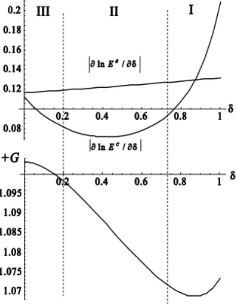
Once we characterize the relative magnitudes of ¯¯∂δ∂ ln Ee¯ and¯ ¯¯∂δ∂ ln Ec¯¯ , we can examine the nonlinear relationship between financial development and economic growth. To better illustrate our analysis, we provide four numerical examples that yield the nonlinear finance-growth rela-tionships consistent with recent empirical studies. Consider the first example where n = 6, λ = 0.7, pb = 0.5, pg = 0.6, εu = 0.18, εg = 0.4, sg = 0.2, Q = 2.3, A = 1.05, α = 0.36, x = 3, z = 0.5, m = 2.2,and μ = 0.67. In this example, δcR is equal to 1.0 while δeR is equal to 2.3. For both types of loans to appear, we should condier the intermediation cost δ that lies between 0 and
Figure 3: Financial development,¯¯∂ ln E∂δ e¯¯ , ¯¯∂ ln E∂δ c¯¯ , and economic growth: the first example 1.0. The loci of¯¯∂ ln E∂δ e¯¯ and¯¯∂ ln E∂δ c¯¯ as functions of δ under this economy for δ ≤ 1.0 is depicted in Figure 1.c and 2.c, which are replicated in the upper half of Figure 3. The corresponding rate of economic growth is depicted in the lower half of Figure 3. Recall that financial development increases (resp. decreases) economic growth if¯¯∂ ln E∂δ e¯¯ > (resp. <)¯¯∂ ln E∂δ c¯¯ . As shown, the effect of financial development on economic growth is uncertain for high levels of δ (i.e., in regime I of Figure 3). For middle levels of δ (i.e., for δ in regime II),¯¯∂ ln Ee
∂δ ¯ ¯ overwhelmingly denominates ¯ ¯∂ ln Ec ∂δ ¯
¯ ; thus, financial development significantly promotes growth. For low levels of δ (i.e., for δ in regime III),¯¯∂ ln E∂δ e¯¯ still dominates ¯¯∂ ln E∂δ c¯¯ so that financial development has a positive effect on growth. Nevertheless, since ¯¯∂ ln E∂δ c¯¯ is increasing in financial development (i.e., ¯¯∂ ln E∂δ c¯¯ is decreasingg in δ) in regime III, the positive effect of financial development on growth in regime III is less significant than that in regime II. Obviously, this example replicates the empirical result found by Rioja and Valev (2004).
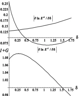
In the second example, pb = 0.42, εu = 0.15, εg = 0.38, A = 0.88, α = 0.25,and μ = 0.65. All other exogenous variables are identical to the first example. In this example,¯¯∂ ln Ee
∂δ ¯ ¯ and¯¯∂ ln Ec ∂δ ¯ ¯ are depicted in the upper half of Figure 4 while the correlation between economic growth and δ is depicted in the lower half of Figure 4. As shown,¯¯∂ ln E∂δ e¯¯ > (<)¯¯∂ ln E∂δ c¯¯ for δ > (<)0.268. Thus,
Figure 4: Financial development,¯¯∂ ln E∂δ e¯¯ ,¯¯∂ ln E∂δ c¯¯ , and economic growth: the second example the relationship between financial development and economic growth is an inverse-U shape. Financial development first promotes growth for low levels of financial development (i.e., for δ > 0.268). For high levels of financial development (i.e., for δ < 0.268), financial development reduces economic growth. This example is consistent with Shen and Lee (2006).
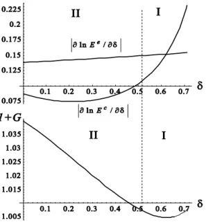
In the third example, εu = 0.25, A = 0.95, α = 0.4, and all other variables are identical to the first example. In this example,¯¯∂ ln E∂δ e¯¯ and ¯¯∂ ln E∂δ c¯¯ are depicted in the upper half of Figure 5 while the correlation between economic growth and δ is depicted in the lower half of Figure 5. Because financial markets are more developed in high income countries than in low income countries, regime I (defined in Figure 5) corresponds to low income countries, while regime II refers to high income countries. Apparently, financial development has an ambiguous effect on economic growth for low income countries, but has a significantly positive effect on growth for high income countries. As a result, this example accords well with the empirical result by Deidda and Fattouh (2002).
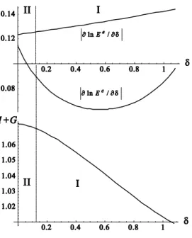
Finally, pb = 0.42, εg = 0.38, εu = 0.15, A = 1.2, α = 0.38, μ = 0.65 in the fourth example and all other variables are the same as in the first example. Figure 6 is the corresponding
Figure 5: Financial development,¯¯∂ ln Ec ∂δ ¯ ¯ , ¯¯∂ ln Ee ∂δ ¯
¯ , and economic growth: the third example figure for this example. As shown, financial development always promotes economic growth. Nevertheless, the marginal effect of financial development on economic growth is bigger in regime I (defined in Figure 6) than in regime II. As regime I corresponds to low and middle income countries, while regime II refers to high income countries, the fourth example indicates that the effect of financial development on economic growth is more significant in low and middle income countries than in high income countries. This result captures the empirical findings of De Gregorios and Guidotti (1995).
6
Conclusion
Recent empirical studies have discovered various nonlinear relationships between financial de-velopment and economic growth. Theoretical models in the recent literature, however, fail to account for all nonlinear finance-growth relationships found by recent empirical studies. To account for this nonlinear relationship, this paper develops a model that incorporates non-productive consumption loans with non-productive investment loans in a standard model of asym-metric information.
Figure 6: Financial development, ¯¯∂ ln E∂δ e¯¯ ,¯¯∂ ln E∂δ c¯¯ , and economic growth: the fourth example In this model, financial development facilitates both investment loans and consumption loans. While facilitating investment loans benefits economic growth, facilitating consumption loans impedes economic growth. As a result, the effect of financial development on economic growth depends on the relative magnitudes of these two distinct channels. It is found that the initial level of financial development (i.e. the initial level of intermediation cost) plays a key role in determining the relative magnitudes of these two channels, yielding nonliear relationships between financial development and economic growth. In particular, we show that integrating consumption loans with investment loans can replicate nonliear relaitonships between financial development and economic growth found by recent empirical works. This highlights the importance of this paper.
References
[1] Bencivenga,V.R. and Smith, B.D., 1991, Financial intermediation and endogenous growth, Review of Economic Studies, 58, pp. 195-209.
[2] Bencivenga,V.R. and Smith, B.D., 1993, Some consequences of credit rationing in an endogenous growth model, Journal of Economic Dynamics and Control, 17, pp. 97-122. [3] Bose, N. and Cothren, R., 1996, Equilibrium loan contracts and endogenous growth in
the presence of asymmetric information, Journal of Monetary Economics, 38, pp. 363-376. [4] Bose, N. and Cothren, R., 1997, Asymmetric information and loan contracts in a
neo-classical growth model, Journal of Money, Credit, and Banking, 29, pp. 423-439.
[5] Capasso, S. and Mavrotas, G., 2003, Loan processing costs and information asymmetries — Implications for financial sector development and economic growth, Discussion Paper No. 2003/84, United Nations University — World Institute for Development Economics Research. [6] De Gregorio, J. and Guidotti, P., 1995, Financial development and economic growth,
World Development, 23, pp. 433-448.
[7] Deidda, L., 2006, Interaction between economic growth and financial development, Jour-nal of Monetary Economics, 53, pp. 233-248.
[8] Deidda, L. and Fattouh, B., 2002, Nonlinearity between finance and growth, Economics Letters, 74, 339-345.
[9] Diamond, D.W., 1984, Financial intermediation and delegated monitoring, Review of Economic Studies, 51, pp. 393-414
[10] Fry, M.J., 1995, Money, Interest, and Banking in Economic Development. 2nd ed. Balti-more: Johns Hopkins University Press.
[11] Goldsmith, R.W., 1969, Financial Structure and Development. New Haven, CT: Yale University Press.
[12] Greenwood, J. and Jovanovic, B., 1990, Financial development, growth, and the dis-tribution of income, Journal of Political Economy, 98, pp. 1076-1107.
[13] Ho, W.-H. and Wang, Y., 2005, Public capital, asymmetric information, and economic growth, Canadian Journal of Economics, 38, pp. 57-79.
[14] Jappelli, T. and Pagano, M., 1994, Saving, growth, and liquidity constraints, Quarterly Journal of Economics, 109, pp. 83-109.
[15] King, R.G. and Levine, R., 1993a, Finance and growth: Schumpeter might be right, Quarterly Journal of Economics, 108, pp. 717-738.
[16] King, R.G. and Levine, R., 1993b, Finance, entrepreneurship, and growth–theory and evidence, Journal of Monetary Economics, 32, pp. 513-542.
[17] Levine, R. Loayza, N, and Beck, T., 2000, Financial intermediation and growth: causal-ity and causes, Journal of Monetary Economics, 46, pp. 31-77.
[18] Levine, R., 2004, Finance and Growth: Theory and Evidence, No 10766, NBER Working Papers.
[19] McKinnon, R.I., 1973, Money and Capital in Economic Development. Washington, DC: Brookings Institution.
[20] Rioja, F. and Valev, N., 2004, Does one size fit all? A reexamination of the finance and growth relationship, Journal of Development Economics, 74, pp. 429-447.
[21] Saint-Paul, G., 1992, Technological choice, financial markets and economic development, European Economic Review, 36, pp. 763-781.
[22] Shaw, E., 1973, Financial Deepening in Economic Development. New York: Oxford Uni-versity Press.
[23] Shen, C.H. and Lee, C.C., 2006, Same financial development yet different economic growth—why? Journal of Money, Credit, and Banking, 38, pp. 1907-1944.