支持向量模糊類神經網路及其在資料分類和函數近似之應用

(1)

國立交通大學

電機與控制工程學系

博

士

論

文

支持向量模糊類神經網路及其在資料分類和函

數近似之應用

Support-Vector based Fuzzy Neural Networks

and its Applications to Pattern Classification and

Function Approximation

研究生：葉長茂

指導教授：林進燈

(2)

支持向量模糊類神經網路及其在資料分類和

函數近似之應用

Support-Vector based Fuzzy Neural Networks and its Applications

to Pattern Classification and Function Approximation

研究生：葉長茂 Student：Chang-Mao Yeh

指導教授：林進燈博士

Advisor：Dr. Chin-Teng Lin

國立交通大學

電機與控制工程學系

博士論文

A Dissertation

Submitted to Department of Electrical and Control Engineering

College of Electrical Engineering and Computer Science

National Chiao Tung University

in partial Fulfillment of the Requirements

for the Degree of

Doctor of Philosophy

in

Electrical and Control Engineering

September 2006

Hsinchu, Taiwan, Republic of China

(3)

支持向量模糊類神經網路及其在資料分類和函

數近似之應用

摘要

模糊類神經網路經常使用倒傳遞學習演算法或分群學習演算法學習調整模糊規則和歸屬函數的參數以解決資料分類和函數回歸等問題，但是此學習演算法經常不能將訓練誤差及預測誤差同時地最小化，這將造成在資料分類之預測階段無法達到最好的分類效能，且對含有雜訊的訓練資料進行回歸近似時，常有過度訓練而造成回歸效能大大降低的問題。本論文結合支持向量學習機制與模糊類神經網路的優點，提出一個新的支持向量模糊類神經網路(SVFNNs)，此 SVFNNs 將高維度空間具有極優越分類能力的支持向量機(SVM)和極優越強健抗雜訊能力的支持向量回歸(SVR)與能夠有效處理不確定環境資訊的類似人類思考的模糊類神經網路之優點結合。首先我們提出一個適應模糊核心函數(adaptive fuzzy kernel)，進行模糊法則建構，此模糊核心函數滿足支持向量學習所須之默塞爾定理(Mercer’s theorem)， SVFNNs 的學習演算法有參個學習階段，在第一個階段，藉由分群原理自動產生模糊規則和歸屬函數，在第二階段，利用具有適應模糊核心函數之 SVM 和 SVR 來計算模糊神經網路的參數，最後在第三階段，透過降低模糊規則的方法來移除不重要的模糊規則。我們將 SVFNNs 應用到 Iris、Vehicle、Dna、Satimage、Ijcnn1 五個資料集和兩個單變數及雙變數函數進行資料分類與函數近似應用，實驗結果顯示我們提出的 SVFNNs 能在使用較少的模糊規則下有很好的概化(generalization)之資料分類效能和強健抗雜訊的函數近似效能。

(4)

Support-Vector based Fuzzy Neural Networks and its

Applications to Pattern Classification and Function

Approximation

Student: Chang-Mao Yeh Advisor: Chin-Teng Lin

Department of Electrical and Control Engineering National Chiao-Tung University

Abstract

Fuzzy neural networks (FNNs) have been proposed and successfully applied to solving these problems such as classification, identification, control, pattern recognition, and image processing, etc. Fuzzy neural networks usually use the backpropagation or C-cluster type learning algorithms to learn the parameters of the fuzzy rules and membership functions from the training data. However, such learning algorithm only aims at minimizing the training error, and it cannot guarantee the lowest testing error rate in the testing phase. In addition, the local solutions and slow convergence often impose practical constraints in the function approximation problems

In this dissertation, novel fuzzy neural networks combining with support vector learning mechanism called support-vector based fuzzy neural networks (SVFNNs) are proposed for pattern classification and function approximation. The SVFNNs combine the capability of minimizing the empirical risk (training error) and expected risk (testing error) of support vector learning in high dimensional data spaces and the efficient human-like reasoning of FNN in handling uncertainty information. First, we propose a novel adaptive fuzzy kernel, which has been proven to be a Mercer kernel, to construct initial fuzzy

(5)

rules. A learning algorithm consisting of three learning phases is developed to construct the SVFNNs and train the parameters. In the first phase, the fuzzy rules and membership functions are automatically determined by the clustering principle. In the second phase, the parameters of FNN are calculated by the SVM and SVR with the proposed adaptive fuzzy kernel function for pattern classification and function approximation, respectively. In the third phase, the relevant fuzzy rules are selected by the proposed fuzzy rule reduction method. To investigate the effectiveness of the proposed SVFNNs, they are applied to the Iris、Vehicle、Dna、Satimage and Ijcnn1 datasets for classification, and one- and two- variable functions for approximation, respectively. Experimental results show that the proposed SVFNNs can achieve good pattern classification and function approximation performance with drastically reduced number of fuzzy kernel functions (fuzzy rules).

(6)

誌謝

首先感謝指導教授林進燈院長多年來的指導。在學術上，林教授以其深厚的學識涵養及孜孜不倦的教導，使我在博士研究期間，學到了許多寶貴的知識、研究的態度及解決問題的能力。除了學術上的收穫之外，也相當感謝林教授在日常生活上給予的關心與鼓勵，每當我在最徬徨的時侯，總能指點我正確的方向，在我最失意的時侯，讓我重拾信心，另外林教授的學識淵博、做事衝勁十足、熱心待人誠懇與風趣幽默等特質，都是我非常值得學習的地方。今日之所以能夠順利完成學業，都是老師悉心的教導，在此對林教授獻上最誠摯的敬意。此外亦非常感謝諸位口試委員在論文上所給于的寶貴建議與指教，使得本論文更加完備。在家人方面，首先感謝我的父親葉哲元先生與母親林寶葉女士從小到大對我的教養與栽培，由於您們長年以來的支持與鼓勵，使得我無後顧之憂的專心於學業方面。及感謝我的哥哥長青與妹妹蕙蘭平日對我的關心。同時也感謝我的妻小：維珊和子鴻和芸芸；多年來因為學業的關係，很少陪伴你們，日後當會好好的補償你們。在學校方面，感謝勝富和翊方學長在研究與生活的熱心幫忙，這段一起研究討論的日子，不但讓我學到研究方法，也讓我學到解決問題的能力。及感謝實驗室裡每位學長、學弟及同學在學業及日常的照顧，這段一起唸書、閒話家常的日子，不僅讓我總能抱著愉快的心情學習，更讓我在這求學過程多釆多姿。在工作方面，感謝學校內長官與同事多年來的支持，得以使我能夠順利完成本論文。最後，謹以本論文獻給我的家人與關心我的師長與朋友們。

(7)

LIST OF FIGURES

Fig. 2.1 The structure of the four-layered fuzzy neural network. ... 7 Fig. 2.2 The aligned clustering-based partition method giving both less

number of clusters as well as less number of membership functions. ... 9 Fig. 2.3 The clustering arrangement allowing overlap and selecting the

member points according to the labels (or classes) attached to them. ... 11 Fig 3.1 Optimal canonical separating hyperplane with the largest margin

between the two classes... 20 Fig. 3.2 map the training data nonlinearly into a higher-dimensional feature

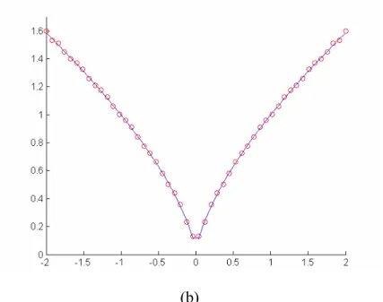
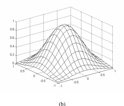
space ... 21 Fig. 4.1 the soft margin loss setting for a regression problem... 37 Fig. 4.2 (a) The desired output of the function show in (4.8). (b) The resulting approximation by SVFNN... 45 Fig 4.3 (a) The desired output of the function show in (4.9) (b) The resulting approximation by SVFNN... 46 Fig 4.4 (a) The desired output of the function show in (4.10). (b) The resulting approximation by SVFNN... 47 Fig 4.5 (a) The desired output of the function show in (4.11). (b) The resulting approximation by SVFNN... 48

(10)

LIST OF TABLES

TABLE 3.1 Experimental results of SVFNN classification on the Iris dataset. ... 32 TABLE 3.2 Experimental results of SVFNN classification on the Vehicle

dataset. ... 32 TABLE 3.3 Experimental results of SVFNN classification on the Dna dataset.

... 33 TABLE 3.4 Experimental results of SVFNN classification on the Satimage

dataset. ... 33 TABLE 3.5 Experimental results of SVFNN classification on the Ijnn1

dataset. ... 34 TABLE 3.6 Classification error rate comparisons among FNN,

RBF-kernel-based SVM, RSVM and SVFNN classifiers, where NA means “not available”... 34 TABLE 4.1 (a) Experimental results of SVFNN on the first function using the training data without noise. (b) Experimental results of SVFNN on the first function using the training data with noise... 51 TABLE 4.2 (a) Experimental results of SVFNN on the second function using the training data without noise. (b) Experimental results of SVFNN on the second function using the training data with noise. ... 52 TABLE 4.3 (a) Experimental results of SVFNN on the third function using the training data without noise. (b) Experimental results of SVFNN on the third function using the training data with noise... 53 TABLE 4.4 (a) Experimental results of SVFNN on the fourth function using

the training data without noise. (b) Experimental results of SVFNN on the fourth function using the training data with noise. ... 54 TABLE 4.5 Comparisons RMSE using the training data without noise... 55 TABLE 4.6 Comparisons RMSE using the training data with noise... 55

(11)

CHAPTER 1 INTRODUCTION

It is an important key issue in many scientific and engineering fields to classify the acquired data or estimate an unknown function from a set of input-output data pairs. As is widely known, fuzzy neural networks (FNNs) have been proposed and successfully applied to solving these problems such as classification, identification, control, pattern recognition, and image processing. most previous researches issue the method of automatically generating fuzzy rules from numerical data and use the backpropagation (BP) and/or C-cluster type learning algorithms to train parameters of fuzzy rules and membership functions from the training data. However, such learning algorithm only aims at minimizing the training error, and it cannot guarantee the lowest testing error rate in the testing phase. In addition, the local solutions and slow convergence often impose practical constraints in the function approximation problems. Therefore, it is desired to develop a novel FNNs, that achieve good pattern classification and function approximation performance with drastically reduced number of fuzzy kernel functions (fuzzy rules).

1.1 Fuzzy Neural Network

Both fuzzy logic and neural networks are aimed at exploiting human-like knowledge processing capability. The fuzzy logic system using linguistic information can model the qualitative aspects of human knowledge and reasoning processes without employing precise quantitative analyses [1]. However, the selection of fuzzy if-then rules often conventionally relies on a substantial amount of heuristic

(12)

observation to express proper strategy’s knowledge. Obviously, it is difficult for human experts to examine all the input-output data to find a number of proper rules for the fuzzy system. Artificial neural networks are efficient computing models which have shown their strengths in solving hard problems in artificial intelligence. The neural networks are a popular generation of information processing systems that demonstrate the ability to learn from training data [2]. However, one of the major criticisms is their being black boxes, since no satisfactory explanation of their behavior has been offered. This is a significant weakness, for without the ability to produce comprehensible decision, it is hard to trust the reliability of networks addressing real-world problems. Much research has been done on fuzzy neural networks (FNNs), which combine the capability of fuzzy reasoning in handling uncertain information and the capability of neural networks in learning from processes [3]-[5]. Fuzzy neural networks are very effective in solving actual problems described by numerical examples of an unknown process. They have been successfully applied to classification, identification, control, pattern recognition, and image processing, etc. In particular, many learning algorithms of fuzzy (neural) have been presented and applied in pattern classification and decision-making systems [6], [7]. Moreover, several researchers have investigated the fuzzy-rule-based methods for function approximation and pattern classification [8]-[15].

A fuzzy system consists of a bunch of fuzzy if-then rules. Conventionally, the selection of fuzzy if-then rules often relies on a substantial amount of heuristic observation to express proper strategy’s knowledge. Obviously, it is difficult for human experts to examine all the input-output data to find a number of proper rules for the fuzzy system. Most pre-researches used the backpropagation (BP) and/or C-cluster type learning algorithms to train parameters of fuzzy rules and membership functions from the training data [16], [17]. However, such learning only aims at

(13)

minimizing the classification error in the training phase, and it cannot guarantee the lowest error rate in the testing phase. Therefore we apply the support vector mechanism with the superior classification power into learning phase of FNN to tackle these problems.

1.2 Support Vector Machine

Support vector machines (SVM) has been revealed to be very effective for general-purpose pattern classification [18]. The SVM performs structural risk minimization and creates a classifier with minimized VC dimension. As the VC dimension is low, the expected probability of error is low to ensure a good generalization. The SVM keeps the training error fixed while minimizing the confidence interval. So, the SVM has good generalization ability and can simultaneously minimize the empirical risk and the expected risk for pattern classification problems. SVM construct a decision plane separating two classes with the largest margin, which is the maximum distance between the closest vector to the hyperplane. In other word, the main idea of a support vector machine is to construct a hyperplane as the decision surface in such a way that the margin of separation between positive and negative examples is maximized. More importantly, an SVM can work very well in a high dimensional feature space. The support vector method can also be applied in regression (functional approximation) problems. When SVM is employed to tackle the problems of function approximation and regression estimation, it is referred as the support vector regression (SVR). SVR can perform high accuracy and robustness for function approximation with noise.

(14)

However, the optimal solutions of SVM rely heavily on the property of selected kernel functions, whose parameters are always fixed and are chosen solely based on heuristics or trial-and-error nowadays. The regular SVM suffers from the difficulty of long computational time in using nonlinear kernels on large datasets which come from many real applications. Therefore, our dissertation proposes a systematical procedure to reduce the support vectors to deal with this problem.

1.3 Research Objectives and Organization of this

dissertation

In this dissertation, novel fuzzy neural networks (FNNs) combining with support vector learning mechanism called support-vector-based fuzzy neural networks (SVFNNs) are proposed for pattern classification and function approximation. The SVFNNs combine the capability of minimizing the empirical risk (training error) and expected risk (testing error) of support vector learning in high dimensional data spaces and the efficient human-like reasoning of FNN in handling uncertainty information. There have been some researches on combining SVM with FNN [19]-[22]. In [19], a self-organizing map with fuzzy class memberships was used to reduce the training samples to speed up the SVM training. The objective of [20]-[22] was on improving the accuracy of SVM on multi-class pattern recognition problems. The overall objective of this dissertation is to develop a theoretical foundation for the FNN using the SVM method. We exploit the knowledge representation power and learning ability of the FNN to determine the kernel functions of the SVM adaptively, and propose a novel adaptive fuzzy kernel function, which has been proven to be a Mercer kernel. The SVFNNs can not only well maintain the classification accuracy,

(15)

but also reduce the number of support vectors as compared with the regular SVM. Organization and objectives of the dissertation are as follows.

In chapter 2, a novel adaptive fuzzy kernel is proposed for combining FNN with SVM. We exploit the knowledge representation power and learning ability of the FNN to determine the kernel functions of the SVM adaptively and develop a novel adaptive fuzzy kernel function. The objective of this chapter is to prove that the adaptive fuzzy kernel conform to the Mercer theory.

In chapter 3, a support-vector based fuzzy neural network (SVFNN) is proposed. This network is developed for solving pattern recognition problem. Compared to conventional neural fuzzy network approaches, the objective of this chapter is to construct the learning algorithm of the proposed SVFNN with simultaneously minimizing the empirical risk and the expected risk for good generalization ability and characterize the proposed SVFNN with good classification performance.

In chapter 4, a support-vector based fuzzy neural network for function approximation is proposed. This network is developed for solving function approximation. The objective of this chapter is to integrate the statistical support vector learning method into FNN and characterize the proposed SVFNN with the capability of good robustness against noise.

The applications and simulated results of the SVFNNs are presented at the ends of Chapter 3 and 4, respectively. Finally, conclusions are made on Chapter 5.

(16)

CHAPTER 2 SUPPORT-VECTOR BASED FUZZY NEURAL

NETWORK AND THE ADAPTIVE FUZZY

KERNEL

In this chapter, adaptive fuzzy kernel is proposed for applying the SVM technique to obtain the optimal parameters of FNN. The adaptive fuzzy kernel provides the SVM with adaptive local representation power, and thus brings the advantages of FNN (such as adaptive learning and economic network structure) into the SVM directly. On the other hand, the SVM provides the advantage of global optimization to the FNN and also its ability to minimize the expected risk; while the FNN originally works on the principle of minimizing only the training error.

2.1 Structure of the FNN

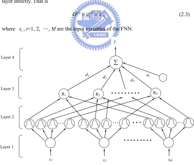
A four-layered fuzzy neural network (FNN) is shown in Fig 2.1, which is comprised of the input, membership function, rule, and output layers. Layer 1 accepts input variables, whose nodes represent input linguistic variables. Layer 2 is to calculate the membership values, whose nodes represent the terms of the respective linguistic variables. Nodes at Layer 3 represent fuzzy rules. The links before Layer 3 represent the preconditions of fuzzy rules, and the link after Layer 3 represent the consequences of fuzzy rules. Layer 4 is the output layer. This four-layered network realizes the following form of fuzzy rules:

(17)

Rule Rj : If x1 is A1j and …xi is Aij….. and xM is AMj, Then y is dj , j=1, 2, …, N, (2.1) where Aij are the fuzzy sets of the input variables xi, i =1, 2, …, M and dj are the consequent parameter of y. For the ease of analysis, a fuzzy rule 0 is added as:

Rule 0 : If x1 is A10 and …….. and xM is AM0, Then y is d0, (2.2) where Ak0 is a universal fuzzy set, whose fuzzy degree is 1 for any input value xi,

i =1, 2, …, M and is the consequent parameter of y in the fuzzy rule 0. Define O

0

d

(P)_{and a}(P)_{as the output and input variables of a node in layer P, respectively. The}

signal propagation and the basic functions in each layer are described as follows. Layer 1- Input layer: No computation is done in this layer. Each node in this layer, which corresponds to one input variable, only transmits input values to the next layer directly. That is

(1) (1)

i

O =a =x_i, (2.3)

where x , i=1, 2, …, M are the input variables of the FNN. _i

Layer 1 Layer 4 Layer 3 Layer 2 d1 dN d2 ∑ x1 x2 d0 xM y R1 R2 RN

(18)

Layer 2 – Membership function layer: Each node in this layer is a membership function that corresponds one linguistic label ( e.g., fast, slow, etc.) of one of the input variables in Layer 1. In other words, the membership value which specifies the degree to which an input value belongs to a fuzzy set is calculated in Layer 2:

, (2.4) (2) ( )j ₍ (2)

i i

O =u a )

M

where is a membership function j=1,

2, …, N. With the use of Gaussian membership function, the operation performed in this layer is ( )j _{( )} i u ⋅ ( )j _{( ) :} _{[0, 1],} _{1, 2,} _, _, i u ⋅ R→ i= ( 2) 2 2 ( ) (2) i ij ij a m O e σ − − = , (2.5)

where mij and σij are, respectively, the center (or mean) and the width (or variance) of the Gaussian membership function of the j-th term of the i-th input variable xi.

Layer 3 – Rule layer: A node in this layer represents one fuzzy logic rule and performs precondition matching of a rule. Here we use the AND operation for each Layer 2 node [ ( )] [ ( )] (3) (3) 1 T j j j j M i i O a e− = =

∏

= D x-m D x-m , (2.6) where 1 1 , , j j M diag σ σ ⎛ ⎞ = _⎜⎜ ⎝ ⎠ D 1 j⎟⎟ , mj=[m1j, m2j, …, mMj]T, x=[x1, x2, x3, …, xM]T is

the FNN input vector. The output of a Layer-3 node represents the firing strength of the corresponding fuzzy rule.

Layer 4 – Output layer: The single node O(4) in this layer is labeled with Σ, which computes the overall output as the summation of all input signals:

(19)

(4) (4) 0 1 N j j j O d a = d =

∑

× + , (2.7)

where the connecting weight dj is the output action strength of the Layer 4 output associated with the Layer 3 rule and the scalar d0 is a bias. Thus the fuzzy neural network mapping can be rewritten in the following input-output form:

. (2.8) (4) (4) ( ) 0 1 1 1 ( ) M N N j j j j i i j j i O d a d d u x = = = =

∑

× + =

∑ ∏

+d₀

2.2 Fuzzy Clustering and Input/Output Space Partitioning

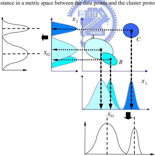
For constructing the initial fuzzy rules of the FNN, the fuzzy clustering method is used to partition a set of data into a number of overlapping clusters based on the distance in a metric space between the data points and the cluster prototypes.

A B C 1 b

x

2 b

x

1

x

2

x

Fig. 2.2 The aligned clustering-based partition method giving both less number of clusters as well as less number of membership functions.

(20)

Each cluster in the product space of the input-output data represents a rule in the rule base. The goal is to establish the fuzzy preconditions in the rules. The membership functions in Layer 2 of FNN can be obtained by projections onto the various input variables x_i spanning the cluster space. In this work, we use an aligned clustering-based approach proposed in [23]. This method produces a partition result as shown in Fig. 2.2.

The input space partitioning is also the first step in constructing the fuzzy kernel function in the SVFNNs. The purpose of partitioning has a two-fold objective:

• It should give us a minimum yet sufficient number of clusters or fuzzy rules.

• It must be in spirit with the SVM-based classification scheme.

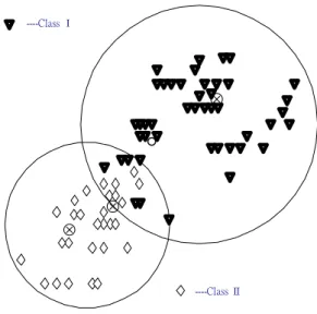
To satisfy the aforementioned conditions, we use a clustering method which takes care of both the input and output values of a data set. That is, the clustering is done based on the fact that the points lying in a cluster also belong to the same class or have an identical value of the output variable. The class information of input data is only used in the training stage to generate the clustering-based fuzzy rules; however, in testing stage, the input data excite the fuzzy rules directly without using class information. In addition, we also allow existence of overlapping clusters, with no bound on the extent of overlap, if two clusters contain points belonging to the same class. We may have a clustering like the one shown in Fig. 2.3. Thus a point may be geometrically closer to the center of a cluster, but it can belong only to the nearest cluster, which has the points belonging to the same class as that point.

(21)

⊗ ⊗ ⊗ ----Class Ⅰ ----Class Ⅱ

Fig. 2.3 The clustering arrangement allowing overlap and selecting the member points according to the labels (or classes) attached to them.

2.3 Fuzzy Rule Generation

A rule corresponds to a cluster in the input space, with mj and Dj representing the center and variance of that cluster. For each incoming pattern x, the strength a rule is fired can be interpreted as the degree the incoming pattern belongs to the corresponding cluster. It is generally represented by calculating degree of membership of the incoming pattern in the cluster [24]. For computational efficiency, we can use the firing strength derived in (2.6) directly as this degree measure

[ ( )] [ ( )] (3) 1 ( ) j j T j j M j i i F a e− = =

∏

= D x-m D x-m x ∈[0,1], (2.9)

where _Fj( )_x _∈

[

0, 1

]

_{. In the above equation the term} _{is the}

distance between x and the center of cluster j. Using this measure, we can obtain the following criterion for the generation of a new fuzzy rule. Let x be the newly incoming pattern. Find

[D x - m_j( _j)] [T D x - m_j( _j)] , (2.10) 1 ( ) arg max j( ) j c t J ≤ ≤ = F x

(22)

where c(t) is the number of existing rules at time t. If _FJ _≤_{F t}( )_{, then a new rule is} generated, where ( ) (0, 1)F t ∈ is a prespecified threshold that decays during the learning process. Once a new rule is generated, the next step is to assign initial centers and widths of the corresponding membership functions. Since our goal is to minimize an objective function and the centers and widths are all adjustable later in the following learning phases, it is of little sense to spend much time on the assignment of centers and widths for finding a perfect cluster. Hence we can simply set

[ ( ) 1]c t + = m x, (2.11) [ ( ) 1] 1 1 1 ln( ) ln( ) c t + _χ diag _FJ _FJ ⎡ ⎤ − = ⋅ _⎢ _⎥ ⎣ ⎦ D , (2.12)

according to the first-nearest-neighbor heuristic [25], where χ ≥0decides the overlap degree between two clusters. Similar methods are used in [26], [27] for the allocation of a new radial basis unit. However, in [26] the degree measure doesn’t take the width Dj into consideration. In [27], the width of each unit is kept at a prespecified constant value, so the allocation result is, in fact, the same as that in [26]. In this dissertation, the width is taken into account in the degree measure, so for a cluster with larger width (meaning a larger region is covered), fewer rules will be generated in its vicinity than a cluster with smaller width. This is a more reasonable result. Another disadvantage of [26] is that another degree measure (the Euclidean distance) is required, which increases the computation load.

After a rule is generated, the next step is to decompose the multidimensional membership function formed in (2.11) and (2.12) to the corresponding 1-D membership function for each input variable. To reduce the number of fuzzy sets of each input variable and to avoid the existence of highly similar ones, we should check the similarities between the newly projected membership function and the existing

(23)

ones in each input dimension. Before going to the details on how this overall process works, let us consider the similarity measure first. Since Gaussian membership functions are used in the SVFNNs, we use the formula of the similarity measure of two fuzzy sets with Gaussian membership functions derived previously in [28].

Suppose the fuzzy sets to be measured are fuzzy sets

A

and

B

with membership

function

{

2 2

}

1 1 ( ) exp ( ) A x x c µ = − − σ and

{

2 2

}

2 2 ( ) exp ( ) B x x c µ = − − σ , respectively.

The union of two fuzzy sets A and B is a fuzzy set A B∪ such that

, for every ( ) max[ ( ), ( )]

A B A B

u _∪ x = u x u x x U∈ . The intersection of two fuzzy sets A

and B is a fuzzy set A B∩ such that u_{A B}_∩ ( ) min[ ( ), ( )]x = u x u x_A _B , for every . The size or cardinality of fuzzy set A, M(A), equals the sum of the support values of A:

x U∈

( ) _A( )

x U

M A u

∈

=

∑

x . Since the area of the bell-shaped function, exp{₋₍_x₋_m₎2_/_σ2}, is σ π [29] and its height is always 1, it can be approximated by an isosceles triangle with unity height and the length of bottom edge 2σ π . We can then compute the fuzzy similarity measure of two fuzzy sets with such kind of membership functions. Assume c₁≥c₂ as in [28], we can compute M A B∩ by

2 2 2 1 1 2 2 1 1 2 1 2 2 1 2 2 1 1 2 1 2 ( ) ( 1 1 (min[ ( ), ( )]) 2 ( ) 2 ( ) ( ) 1 , 2 ( ) A B x U h c c h c c M A B u x u x h c c π σ σ π σ σ π σ σ π σ σ π σ σ π σ σ ∈ ) ⎡ − + + ⎤ ⎡ − + − ⎤ ⎣ ⎦ ⎣ ∩ = = + + − ⎡ − − + ⎤ ⎣ ⎦ + −

∑

⎦ (2.13)

where h( ) max{0, }⋅ = ⋅ . So the approximate similarity measure is

1 2 ( , ) M A B M A B E A B M A B σ π σ π M A B ∩ ∩ = = ∪ + − ∩ , (2.14)

where we use the fact that M A( )+M B( )=M A B( ∩ )+M A B( ∪ ) [28]. By using this similarity measure, we can check if two projected membership functions are close enough to be merged into one single membership

(24)

function

{

2 2

}

3 3

( ) exp ( )

c x x c

µ = − − σ . The mean and variance of the merged

membership function can be calculated by

1 2 3 2 c c c = + , (2.15) 1 3 2 2 σ σ σ = + . (2.16)

2.4 Adaptive Fuzzy Kernel for the SVM/SVR

The proposed fuzzy kernel K( zxˆ,ˆ) in this dissertation is defined as

( )

=1

( ) ( )

, if and are both in the -th cluster , 0, otherwise, M j i j i i u x u z j K ⎧ _⋅ ⎪ =⎨ ⎪⎩

∏

x z x z (2.17)

where x =[x1, x2, x3, …, xM] ∈RM and =[zz 1, z2, z3, …, zM] ∈RM are any two training samples, and u x is the membership function of the j-th cluster. Let the _j

( )

_i

training set be S={(x1, y1), (x2, y2), …, (xv, yv)} with explanatory variables and the corresponding class labels y

i

x

i, for all i=1, 2, , v, where v is the total number of training samples. Assume the training samples are partitioned into l clusters through fuzzy clustering in Section II. We can perform the following permutation of training samples

(

)

(

)

{

}

(

)

(

)

{

}

(

)

(

)

{

}

1 2 1 1 1 2 2 1 1 1 , , , , 2 , , , , , , , , l k k l l l k cluster y y cluster y y cluster l y y = = = x x x x x x … … … 1 2 l 1 1 1 k 2 2 1 k l 1 k , ,l (2.18)

(25)

that we have 1 l g g k =

∑

= v. Then the fuzzy kernel can be calculated by using the training set in (2.18), and the obtained kernel matrix K can be rewritten as the following form

1 2 v v l R × ⎡ ⎤ ⎢ ⎥ ⎢ = ⎢ ⎢ ⎥ ⎢ ⎥ ⎣ ⎦ K 0 0 0 K K 0 0 0 K ⎥ ∈ ⎥ ,l (2.19) where Kg, g=1, 2, is defined as

(

)

(

)

(

)

(

)

(

)

(

)

(

)

(

) (

)

1 1 1 2 1 2 1 2 2 1 1 1 , , , , , , , , , g g g g g g g g g g g g g g g g k g g g g k k g _g _g k k g g g g g g k k k k k K x x K x x K x x K x x K x x R K x x K x x K x x K x x × − − ⎡ ⎤ ⎢ ⎥ ⎢ ⎥ ⎢ ⎥ =_⎢ _⎥∈ ⎢ ⎥ ⎢ ⎥ ⎢ ⎥ ⎣ ⎦ K (2.20)

In order that the fuzzy kernel function defined by (2.17) is suitable for application in SVM, we must prove that the fuzzy kernel function is symmetric and positive-definite Gram Matrices [30]. To prove this, we first quote the following theorems.

Theorem 1 (Mercer theorem [30]) : Let X be a compact subset of Rn. Suppose K

is a continuous symmetric function such that the integral operator TK : L2(X)→L2(X)

( ) ( )

( _K )( ) 0 X T f ⋅ =

∫

K ⋅, x f x dx≥ , (2.21) is positive; that is

(

) ( ) ( )

0, 2( ) X X K f f d d f L × ≥ ∀ ∈

∫

x, z x z x z X (2.22)

for all f ∈L X₂( ). Then we can expand K(x, z) in a uniformly convergent series

(on X X× ) in terms of TK’s eigen-functions φj∈L X2( ), normalized in such a way that

2

1 j L

(26)

. (2.23)

(

)

( ) (

1 j j j j K ∞ λ φ φ = =

∑

x, z x z

)

The kernel is referred to as Mercer’s kernel as it satisfies the above Mercer theorem.

Proposition 1 [31] : A function K(x, z) is a valid kernel iff for any finite set it

produces symmetric and positive-definite Gram matrices.

Proposition 2 [32] : Let K1 and K2 be kernels over X X× , . Then the function is also a kernel.

n

X ⊆R

1 2

( ( (

K x, z)=K x, z)K x, z)

Definition 1 [33] : A function is said to be a positive-definite

function if the matrix

:

f R→R

[ ( )] n n

i j

f x −x ∈R × is positive semidefinite for all choices of points { , , }x₁ x_n ⊂ R and all n=1, 2, .

Proposition 3 [33] : A block diagonal matrix with the positive-definite diagonal

matrices is also a positive-definite matrix.

Theorem 2 : For the fuzzy kernel defined by (2.17), if the membership functions

are positive-definite functions, then the fuzzy kernel is a Mercer kernel.

( )

_i : [0, 1], 1, 2, ,

u x R→ i= n,

Proof:

First, we prove that the formed kernel matrix

(

)

, 1 = , n i j K = K x xi j is a

symmetric matrix. According to the definition of fuzzy kernel in (2.17), if and are in the j-th cluster,

i x z_i ,

(

)

j

( ) ( )

j j

( ) ( )

j

(

)

k=1 k=1 , n _k _k n _k _k , K x z =

∏

u x ⋅u z =

∏

u z ⋅u x =K z x otherwise, ) , ( zx K =K z x( , )=0.

(27)

So the kernel matrix is indeed symmetric. By the elementary properties of

Proposition 2, the product of two positive-defined functions is also a kernel function.

And according to Proposition 3, a block diagonal matrix with the positive-definite

diagonal matrices is also a positive-definite matrix. So the fuzzy kernel defined by (2.17) is a Mercer kernel.

Since the proposed fuzzy kernel has been proven to be a Mercer kernel, we can apply the SVM technique to obtain the optimal parameters of SVFNNs. It is noted that the proposed SVFNNs is not a pure SVM, so it dose not minimize the empirical risk and expected risk exactly as SVMs do. However, it can achieve good classification performance with drastically reduced number of fuzzy kernel functions.

(28)

CHAPTER 3 SUPPORT-VECTOR BASED FUZZY NEURAL

NETWORK FOR PATTERN CLASSIFICATION

In this chapter, we develop a support-vector-based fuzzy neural network (SVFNN) for pattern classification, which is the realization of a new idea for the adaptive kernel functions used in the SVM. The use of the proposed fuzzy kernels provides the SVM with adaptive local representation power, and thus brings the advantages of FNN (such as adaptive learning and economic network structure) into the SVM directly. On the other hand, the SVM provides the advantage of global optimization to the FNN and also its ability to minimize the expected risk; while the FNN originally works on the principle of minimizing only the training error. The proposed learning algorithm of SVFNN consists of three phases. In the first phase, the initial fuzzy rule (cluster) and membership of network structure are automatically established based on the fuzzy clustering method. The input space partitioning determines the initial fuzzy rules, which is used to determine the fuzzy kernels. In the second phase, the means of membership functions and the connecting weights between layer 3 and layer 4 of SVFNN (see Fig. 2.1) are optimized by using the result of the SVM learning with the fuzzy kernels. In the third phase, unnecessary fuzzy rules are recognized and eliminated and the relevant fuzzy rules are determined. Experimental results on five datasets (Iris, Vehicle, Dna, Satimage, Ijcnn1) from the UCI Repository, Statlog collection and IJCNN challenge 2001 show that the proposed SVFNN classification method can automatically generate the fuzzy rules, improve the accuracy of

(29)

classification, reduce the number of required kernel functions, and increase the speed of classification.

3.1 Maximum Margin Algorithm

An SVM constructs a binary classifier from a set of labeled patterns called training examples. Let the training set be S = {(x1, y1), (x2, y2), …, (xv, yv)} with

explanatory variables and the corresponding binary class labels

, for all , where v denotes the number of data, and d denotes

the dimension of the datasets. The SVM generates a maximal margin linear decision rule of the form

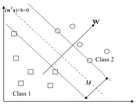
d i∈ x R { 1, 1} i y ∈ − + i=1, ,v ( ) sign( ) f x = w x⋅ +b , (3.1)

Where w is the weight vector and b is a bias. The margin M can be calculated by M=2/||w|| that show in Fig. 3.1. For obtaining the largest margin, the weight vector, ,

must be calculated by

w

_min 1 2

2 w

s.t. (y_i x w_i +b) 1 0,− ≥ ∀ =i 1, ,v. (3.2)

The optimization problem be converted to a quadratic programming problem, which can be formulated as follows:

1 , 1 1 Maximize ( ) 2 α α α α = = =

∑

v −

∑

v T i i j i j i i j L y y x x_i _j subject to α_i ≥ , i = 1, 2,…., v and 0 . (3.3) 1 0 v i i i y α = =

∑

whereαi denotes Lagrange multiplier.

(30)

Class 1

Class 2

M

(wTx)+b=0

Fig 3.1 Optimal canonical separating hyperplane with the largest margin between the two classes.

In practical applications for non-ideal data, the data contain some noise and overlap. The slack variablesξ , which allow training patterns to be misclassified in the case of linearly non-separable problems, and the regularization parameter C, which

sets the penalty applied to margin-errors controlling the trade-off between the width of the margin and training set error, are added to SVM. The equation is altered as follows: _min 1 2 2 2 2 i i C _ξ +

∑

w s.t. (y_i x w_i +b) 1≥ −ξ_i, ∀ =i 1, ,v. (3.4)

To construct a non-linear decision rule, the kernel method mappin an input vector _{x R}_∈ d into a vector of a higher-dimensional feature space F (_φ_{( )}_x _{, where} _φ

represents a mapping d _→ ) is discovered. Therefore, the maximal margin linear

(31)

classifier can solve the linear and non-linear classification problem in this feature space. Fig. 3.2 show the training data map into a higher-dimensional feature space. However, the computation cannot easily map the input vector to the feature space. If the dimension of transformed training vectors is very large, then the computation of the dot products is prohibitively expensive. The transformed function ( )φ x is not _i

known a priori. The Mercer’s theorem provides a solution for those problems. The equation φ( ) ( )x_i ⋅φ x_j can be calculated directly by a positive definite symmetric kernel function K x x( , )i j =φ( ) ( )xi ⋅φ xj which complies with Mercer’s theorem. Popular choices for Kernel function include

Gaussian kernel : 2 2 ( , ) exp( ) 2 K σ − = − x x x x (3.5a)

and Polynomial kernel : 2

2 ( , ) (1 ) K σ ⋅ = + x x x x . (3.5b)

To obtain an optimal hyperplane for any linear or nonlinear space, Eq. (3.4) can be rewritten to the following dual quadratic optimization

max

α

( )

1 1

(

)

1 , 2 α =

∑

v α −

∑

v _i _{j i}α α_j i i, j L _i y y K x x_i _j = = subject to 0≤α_i ≤C i, =1, 2,...,v and . (3.6) 1 0 v i i i y a =

∑

=

Fig.3.2 map the training data nonlinearly into a higher-dimensional feature space

Φ:x→ φ(x)

( , )_i _j ( ) ( )_i _j

(32)

The dual Lagrangian L

( )

α must be maximized with respect toαi≥ 0. The training patterns with nonzero Lagrange multipliers are called support vectors. The separating function is given as follows

0 0 1 ( ) sign α ( ) = ⎛ ⎞ = _⎜ ⎝

∑

⎠ sv N i i i i + ⎟ f x y K x x b . (3.7)

where Nsv denotes the number of support vectors; xi denotes a support vectors; 0

i

α denotes a corresponding Lagrange coefficient, and b0 denotes the constant given by

(

*

) (

* 0 0 0 1 (1) ( 1) 2⎡

)

⎤ = − _⎣ + − _⎦ b w x w x , (3.8)

where x*(1) denote some support vector belonging to the first class and

0≤α_i≤ C. x*_{(−1) denote some support vector belonging to the second class, where}

0≤α_i≤ C. In next section, we proposed the learning algorithm of SVFNN that

combine the capability of minimizing the empirical risk (training error) and expected risk (testing error) of support vector learning in high dimensional data spaces and the efficient human-like reasoning of FNN in handling uncertainty information.

3.2 Learning Algorithm of SVFNN

The learning algorithm of the SVFNN consists of three phases. The details are given below:

Learning Phase 1 – Establishing initial fuzzy rules

The first phase establishes the initial fuzzy rules, which were usually derived from human experts as linguistic knowledge. Because it is not always easy to derive

(33)

fuzzy rules from human experts, the method of automatically generating fuzzy rules from numerical data is issued. The input space partitioning determines the number of fuzzy rules extracted from the training set and also the number of fuzzy sets. We use the centers and widths of the clusters to represent the rules. To determine the cluster to which a point belongs, we consider the value of the firing strength for the given cluster. The highest value of the firing strength determines the cluster to which the point belongs. The whole algorithm for the generation of new fuzzy rules as well as fuzzy sets in each input variable is as follows. Suppose no rules are existent initially.

IF x is the first incoming input pattern THEN do

PART 1. { Generate a new rule with center m = x₁ and width

1 1 1 , , init init diag σ σ ⎛ ⎞ = _⎜ _⎟ ⎝ ⎠ D ,

IF the output pattern y belongs to class 1 (namely, y =[1 0]),

{

wCon−1=[1 0] for indicating output node 1 been excited, }

ELSE { w_Con₋₁=[0 1] for indicating output node 2 been

excited.}

}

ELSE for each newly incoming input , do x

PART 2. {Find as defined in (2.9). 1 (t) arg max j( ), j c J ≤ ≤ = F x IF w_{Con J}₋ ≠ y,

(34)

( 1) c t+ = m x ,

( )

( 1) 1 1 1 , , ln ln c t+ χ diag _FJ _F ⎛ ⎞ − _⎜ _⎟ = ⎜ ⎟ ⎝ ⎠ D _J and , where ( 1) Con c t− + = y

w χ decides the overlap degree between two

clusters. In addition, after decomposition, we have m_{new i}₋ =x_i,

ln( J)

new i F

σ ₋ = − ×χ , i=1, ,M . Do the following fuzzy measure for each input variable i:

{ ( , ) max₁ ( , ), ( , )

i

j k new i new i ij ij

Degree i t ≡ _{≤ ≤} E⎡_⎣µ m ₋ σ ₋ µ m σ ⎤_⎦

, where E(‧) is defined in (2.14). IF Degree i t( , )≤ρ( )t

THEN adopt this new membership function, and set 1

i i

k = + , where k k_i is the number of partitions of the ith input variable.

ELSE merge the new membership function with closest one

2 new i closest new i closest m m m m − − + = = , 2 σ σ σ σ − − + = = new i closest new i closest . } } ELSE {If J ( ) in F ≤F t

{generate a new fuzzy rule with m_{c t}_{( 1)}₊ =x,

( )

( 1) 1 1 1 , , ln ln c t+ _χ diag _FJ _FJ ⎛ − _⎜ = ⎜ ⎟ ⎝ ⎠

D ⎞⎟, and the respective consequent

weight w_{Con a t}₋ _{( 1)}₊ = y. In addition, we also need to do the

(35)

In the above algorithm, σ_init is a prespecified constant, is the rule number at time t,

( )

c t

χ decides the overlap degree between two clusters, and the threshold F_in

determines the number of rules generated. For a higher value of Fin, more rules are generated and, in general, a higher accuracy is achieved. The valueρ is a scalar ( )t

similarity criterion, which is monotonically decreasing such that higher similarity between two fuzzy sets is allowed in the initial stage of learning. The pre-specified values are given heuristically. In general, F(t)=0.35, β =0.05, 5σ_init =0. , χ =2. In addition, after we determine the precondition part of fuzzy rule, we also need to properly assign the consequence part of fuzzy rule. Here we define two output nodes for doing two-cluster recognition. If output node 1 obtains higher exciting value, we know this input-output pattern belongs to class 1. Hence, initially, we should assign

the proper weight for the consequence part of fuzzy rule. The above

procedure gives us means ( ) and variances (

1 Con− w ij m 2 ij σ ) in (2.9). Another parameter in (2.7) that needs concern is the weight dj associated with each . We shall see later in Learning Phase 2 how we can use the results from the SVM method to determine these weights.

(4)

j

a

Learning Phase 2 - Calculating the parameters of SVFNN

Through learning phase (1), the initial structure of SVFNN is established and we can then use SVM [34], [35] to find the optimal parameters of SVFNN based on the proposed fuzzy kernels. The dual quadratic optimization of SVM [36] is solved in order to obtain an optimal hyperplane for any linear or nonlinear space:

(36)

maximize

( )

1

(

,

)

2 L α =

∑

v α_i −

∑

v y y_i _jα α_i _jK x x_i _j i =1 i, j=1 subject to 0≤α_i ≤C i, =1, 2, , v, and 0, (3.9) i=1 yα =

∑

v i i

where is the fuzzy kernel in (2.17) and C is a user-specified positive

parameter to control the tradeoff between complexity of the SVM and the number of nonseparable points. This quadratic optimization problem can be solved and a

solution can be obtained, where

(

, K x xi j

)

(

0 0 0 0 ₁, ₂, ..., _nsv α = α α α 0 i α are Lagrange coefficients, and nsv is the number of support vectors. The corresponding support

vectors can be obtained, and the constant

(threshold) d [ ₁ ₂ , _i, , ] sv = sx , sx , sx sx_nsv 0 in (2.7) is

(

*

) (

* 0 0 0 1 (1) ( 1) 2 d = ⎡_⎣ w x⋅ + w x⋅ −

)

₀ 1 nsv i i i i w α y x = =

∑

⎤⎦ with , (3.10)

where nsv is the number of fuzzy rules (support vectors); the support vector x*₍₁₎ belongs to the first class and support vector x*(-1) belongs to the second class. Hence, the fuzzy rules of SVFNN are reconstructed by using the result of the SVM learning with fuzzy kernels. The means and variances of the membership functions can be calculated by the values of support vector m_j =sx_j, j=1, 2, …, nsv, in (2.5) and (2.6)

and the variances of the multidimensional membership function of the cluster that the support vector belongs to, respectively. The coefficients dj in (2.7) corresponding to

j = j

m sx can be calculated by d_j = y_jα_j. In this phase, the number of fuzzy rules can be increased or decreased. The adaptive fuzzy kernel is advantageous to both the SVM and the FNN. The use of variable-width fuzzy kernels makes the SVM more efficient in terms of the number of required support vectors, which are corresponding to the fuzzy rules in SVFNN.

(37)

Learning Phase 3 – Removing irrelevant fuzzy rules

In this phase, we propose a method for reducing the number of fuzzy rules learning in Phases 1 and 2 by removing some irrelevant fuzzy rules and retuning the consequent parameters of the remaining fuzzy rules under the condition that the classification accuracy of SVFNN is kept almost the same. Several methods including orthogonal least squares (OLS) method and singular value decomposition QR (SVD-QR) had been proposed to select important fuzzy rules from a given rule base [37]-[39]. In [37] the SVD-QR algorithm select a set of independent fuzzy basis function that minimize the residual error in a least squares sense. In [38], an orthogonal least-squares method tries to minimize the fitting error according to the error reduction ratio rather than simplify the model structure [39]. The proposed method reduces the number of fuzzy rules by minimizing the distance measure between original fuzzy rules and reduced fuzzy rules without losing the generalization performance. To achieve this goal, we rewrite (2.8) as

2 2 ( ) (4) (4) 0 1 1 1 i ij ij x m M N N j j j j j i O d a d d e σ − − = = = =

∑

× + =

∑ ∏

+d , ₀ (3.11) where N is the number of fuzzy rules after Learning phases 1 and 2. Now we try to approximate it by the expansion of a reduced set :

2 Re 2 Re ( ) Re(4) Re(4) 0 0 1 1 1 i iq z z iq x m R R M q q q q q i O β a d β e σ d − − = = = =

∑

× + =

∑ ∏

+ and 2 Re Re 2 ( ) Re(4) 1 ( ) i iq iq x m M q i a e σ − − = =

∏

x (3.12)

where Rz is the number of reducing fuzzy rules with N> Rz, β is the consequent q

parameters of the remaining fuzzy rules, and Re and

iq

m Re

iq

σ are the mean and

(38)

2 (4) Re(4) (4) Re(4) Re (4) Re , 1 , 1 1 1 ( ) z ( ) 2 z ( R R N N j q j q j q j q j q j q j q j q j q O O d d a β β a d β a = = = = − =

∑

× × m +

∑

× × m − ×

∑∑

× × m ), (3.13)

where . Evidently, the problem of finding reduced fuzzy

rules consists of two parts: one is to determine the reduced fuzzy rules and the other is to compute the expansion coefficients

Re Re Re Re 1 2 [ , , , ]T q = mq m q mMq m i

β . This problem can be solved by choosing

the more important Rz fuzzy rules from the old N fuzzy rules. By adopting the

sequential optimization approach in the reduced support vector method in [41], the approximation in (3.4) can be achieved by computing a whole sequence of reduced set approximations Re(4) Re(4) 1 r r q q

O

β

=

∑

×

a

_q _{, (3.14)}

for r=1, 2, …, RZ. Then, the mean and variance parameters, mReq and σqRe, in

the expansion of the reduced fuzzy-rule set in (3.4) can be obtained by the following iterative optimization rule [41] :

(4) Re 1 Re 1 (4) Re 1 ( ) ( ) N j j q j q N j j q j d a d a = + = × × = ×

∑

m m m m j . (3.15)

According to (3.7), we can find the parameters, Re and q

m Re

q

σ , corresponding

to the first most important fuzzy rule and then remove this rule from the original fuzzy rule set represented by mj, j=1, 2, …, N and put (add) this rule into the reduced fuzzy rule set. Then the procedure for obtaining the reduced rules is repeated. The

optimal coefficients βq, q=1, 2, , Rz, are then computed to approximate

by [41], and can be obtained as

(4) 1 N j j O d = =

∑

×a_j Re(4) aRe 1 z R q q q O β = =

∑

×

(39)

, (3.16) 1 1 2 [ , ..., _R_z] _{R R}_z _z _{R N}_z β β β β − × × = =K ×K × Θ z z R R a m z R mN where

Re(4) Re Re(4) Re Re(4) Re

1 1 1 2 1

Re(4) Re Re(4) Re

2 1 2 2

Re(4) Re 1

Re(4) Re Re(4) Re Re(4) Re

1 1 ( ) ( ) ( ) ( ) ( ) ( ) ( ) ( ) ( ) z z z z z z z z R R R R R R R R a a a a a a a a × − − ⎛ ⎞ ⎜ ⎟ ⎜ ⎟ = ⎜ ⎟ ⎜ ⎟ ⎜ ⎟ ⎝ ⎠ m m m m m K m m m (3.17) and

Re(4) Re(4) Re(4)

1 1 1 2 1

Re(4) Re(4)

2 1 2 2

Re(4) 1

Re(4) Re(4) Re(4)

1 1 ( ) ( ) ( ) ( ) ( ) ( ) ( ) ( ) ( ) x z z z z R R N R N R R N a a a a a a a a a × − − ⎛ ⎞ ⎜ ⎟ ⎜ ⎟ = ⎜ ⎟ ⎜ ⎟ ⎜ ⎟ ⎝ ⎠ m m m m m K m m m (3.18) and 1 2

[ , , ,

d d

d

_N

]

Θ =

. (3.19)

The whole learning scheme is iterated until the new rules are sufficiently sparse.

3.3 Experimental Results

The classification performance of the proposed SVFNN is evaluated on five well-known benchmark datasets. These five datasets can be obtained from the UCI repository of machine learning databases [42] and the Statlog collection [43] and IJCNN challenge 2001 [44], [45], respectively.

A. Data and Implementation

(40)

collection we choose three datasets: Vehicle, Dna and Satimage datasets. The problem Ijcnn1 is from the first problem of IJCNN challenge 2001. These five datasets will be used to verify the effectiveness of the proposed SVFNN classifier. The first dataset (Iris dataset) is originally a collection of 150 samples equally distributed among three classes of the Iris plant namely Setosa, Verginica, and Versicolor. Each sample is represented by four features (septal length, septal width, petal length, and petal width) and the corresponding class label. The second dataset (Vehicle dataset) consists of 846 samples belonging to 4 classes. Each sample is represented by 18 input features. The third dataset (Dna dataset) consists of 3186 feature vectors in which 2000 samples are used for training and 1186 samples are used for testing. Each sample consists of 180 input attributes. The data are classified into three physical classes. All Dna examples are taken from Genbank 64.1. The four dataset (Satimage dataset) is generated from Landsat Multispectral Scanner image data. In this dataset, 4435 samples are used for training and 2000 samples are used for testing. The data are classified into six physical classes. Each sample consists of 36 input attributes. The five dataset (Ijcnn1 dataset) consists of 22 feature vectors in which 49990 samples are used for training and 45495 samples are used for testing. Each sample consists of 22 input attributes. The data are classified into two physical classes. The computational experiments were done on a Pentium III-1000 with 1024MB RAM using the Linux operation system.

For each problem, we estimate the generalized accuracy using different cost parameters C=[212, 211, 210, …, 2-2] in (3.1). We apply 2-fold cross-validation for 100 times on the whole training data in Dna, Satimage and Ijcnn1, and then average all the results. We choose the cost parameter C that results in the best average cross-validation rate for SVM training to predict the test set. Because Iris and Vehicle datasets don’t contain testing data explicitly, we divide the whole data in Iris and

(41)

Vehicle datasets into two halves, for training and testing datasets, respectively. Similarly, we use the above method to experiment. Notice that we scale all training and testing data to be in [-1, 1].

B. Experimental Results

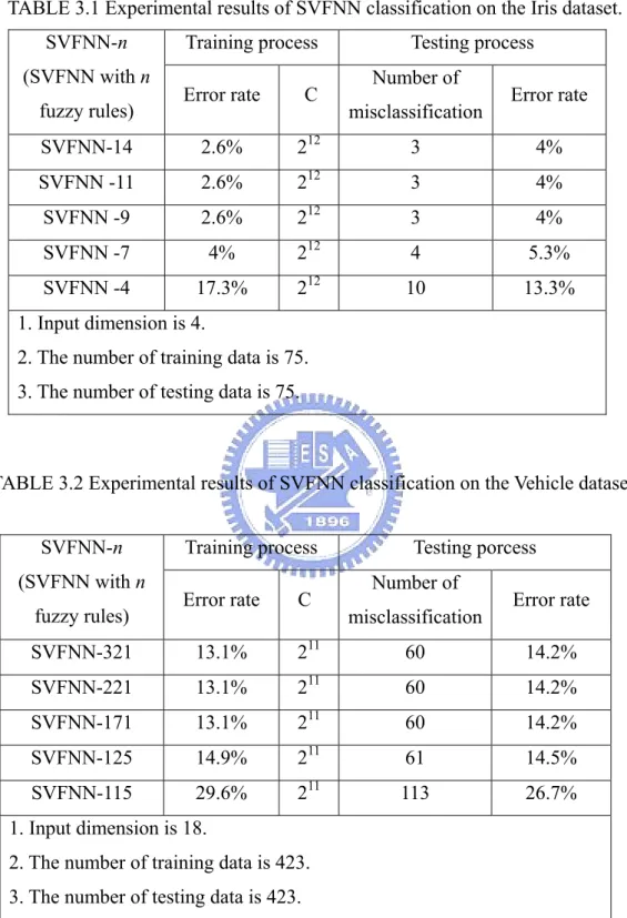
Tables 3.1 to 3.5 present the classification accuracy rates and the number of used fuzzy rules (i.e., support vectors) in the SVFNN on Iris, Vehicle, Dna, Satimage and Ijcnn1 datasets, respectively. The criterion of determining the number of reduced fuzzy rules is the difference of the accuracy values before and after reducing one fuzzy rule. If the difference is larger than 0.5%, meaning that some important support vector has been removed, then we stop the rule reduction. In Table 3.1, the SVFNN is verified by using Iris dataset, where the constant n in the symbol SVFNN-n means the number of the learned fuzzy rules. The SVFNN uses fourteen fuzzy rules and achieves an error rate of 2.6% on the training data and an error rate of 4% on the testing data. When the number of fuzzy rules is reduced to seven, its error rate increased to 5.3%. When the number of fuzzy rules is reduced to four, its error rate is increased to 13.3%. Continuously decreasing the number of fuzzy rules will keep the error rate increasing. From Table 3.2 to 3.5, we have the similar experimental results as those in Table 3.1.

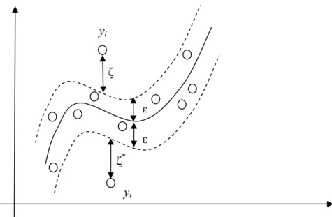
These experimental results show that the proposed SVFNN is good at reducing the number of fuzzy rules and maintaining the good generalization ability. Moreover, we also refer to some recent other classification performance include support vector machine and reduced support vectors methods [46]-[48]. The performance comparisons among the existing fuzzy neural network classifiers [49], [50], the RBF-kernel-based SVM (without support vector reduction) [46], reduced support vector machine (RSVM) [48] and the proposed SVFNN are made in Table 3.6.

(42)

TABLE 3.1 Experimental results of SVFNN classification on the Iris dataset.

Training process Testing process

SVFNN-n (SVFNN with n

fuzzy rules) Error rate C

Number of

misclassification Error rate

SVFNN-14 2.6% 212 3 4% SVFNN -11 2.6% 212 3 4% SVFNN -9 2.6% 212 _{3 4%} SVFNN -7 4% 212 4 5.3% SVFNN -4 17.3% 212 10 13.3% 1. Input dimension is 4.

2. The number of training data is 75. 3. The number of testing data is 75.

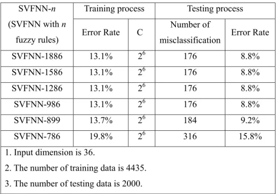
TABLE 3.2 Experimental results of SVFNN classification on the Vehicle dataset.

Training process Testing porcess

Number of

SVFNN-321 13.1% 211 60 14.2% SVFNN-221 13.1% 211 60 14.2% SVFNN-171 13.1% 211 60 14.2% SVFNN-125 14.9% 211 61 14.5% SVFNN-115 29.6% 211 113 26.7% 1. Input dimension is 18.

(43)

TABLE 3.3 Experimental results of SVFNN classification on the Dna dataset.

fuzzy rules) Error Rate C

Number of

SVFNN-904 6.2% 24 64 5.4% SVFNN-704 6.2% 24 64 5.4% SVFNN-504 6.2% 24 64 5.4% SVFNN-334 6.4% 24 69 5.8% SVFNN-300 9.8% 24 139 11.7% 1. Input dimension is 180.

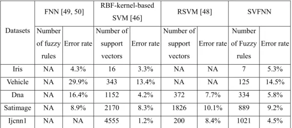
TABLE 3.4 Experimental results of SVFNN classification on the Satimage dataset.

fuzzy rules) Error Rate C

Number of

misclassification Error Rate

SVFNN-1886 13.1% 26 176 8.8% SVFNN-1586 13.1% 26 176 8.8% SVFNN-1286 13.1% 26 176 8.8% SVFNN-986 13.1% 26 176 8.8% SVFNN-899 13.7% 26 184 9.2% SVFNN-786 19.8% 26 316 15.8% 1. Input dimension is 36.

(44)

TABLE 3.5 Experimental results of SVFNN classification on the Ijnn1 dataset.

Training process Testing porcess

Number of

SVFNN-1945 4.2% 212 1955 4.3% SVFNN-1545 4.2% 212 1955 4.3% SVFNN-1245 4.2% 212 1955 4.3% SVFNN-1021 4.3% 212 2047 4.5% SVFNN-977 14.5% 212 _{7416 16.3%} 1. Input dimension is 22.

TABLE 3.6 Classification error rate comparisons among FNN, RBF-kernel-based SVM, RSVM and SVFNN classifiers, where NA means “not available”.

FNN [49, 50] RBF-kernel-based SVM [46] RSVM [48] SVFNN Datasets Number of fuzzy rules Error rate Number of support vectors Error rate Number of support vectors Error rate Number of Fuzzy rules Error rate Iris NA 4.3% 16 3.3% NA NA 7 5.3% Vehicle NA 29.9% 343 13.4% NA NA 125 14.5% Dna NA 16.4% 1152 4.2% 372 7.7% 334 5.8% Satimage NA 8.9% 2170 8.3% 1826 10.1% 889 9.2% Ijcnn1 NA NA 4555 1.2% 200 8.4% 1021 4.5%

支持向量模糊類神經網路及其在資料分類和函數近似之應用

國 立 交 通 大 學

電機與控制工程學系

博

士

論

文

支持向量模糊類神經網路及其在資料分類和函

數近似之應用

Support-Vector based Fuzzy Neural Networks

and its Applications to Pattern Classification and

Function Approximation

研 究 生：葉 長 茂

指導教授：林 進 燈

支持向量模糊類神經網路及其在資料分類和

函數近似之應用

Support-Vector based Fuzzy Neural Networks and its Applications

to Pattern Classification and Function Approximation

研 究 生：葉長茂 Student：Chang-Mao Yeh

指導教授：林進燈 博士

Advisor：Dr. Chin-Teng Lin

國 立 交 通 大 學

電 機 與 控 制 工 程 學 系

博 士 論 文

A Dissertation

Submitted to Department of Electrical and Control Engineering

College of Electrical Engineering and Computer Science

National Chiao Tung University

in partial Fulfillment of the Requirements

for the Degree of

Doctor of Philosophy

in

Electrical and Control Engineering

September 2006

Hsinchu, Taiwan, Republic of China

支持向量模糊類神經網路及其在資料分類和函

數近似之應用

摘 要

Support-Vector based Fuzzy Neural Networks and its

Applications to Pattern Classification and Function

Approximation

Abstract

誌 謝

CONTENTS

LIST OF FIGURES

LIST OF TABLES

CHAPTER 1

INTRODUCTION

1.1 Fuzzy Neural Network

1.2 Support Vector Machine

1.3 Research Objectives and Organization of this

dissertation

CHAPTER 2

SUPPORT-VECTOR BASED FUZZY NEURAL

NETWORK AND THE ADAPTIVE FUZZY

KERNEL

2.1 Structure of the FNN

∏

∑

∑

∑ ∏

2.2 Fuzzy Clustering and Input/Output Space Partitioning

x

x

x

x

2.3 Fuzzy Rule Generation

∏

[

]

A

B

{

}

{

}

∑

∑

{

}

國立交通大學

研究生：葉長茂

指導教授：林進燈

研究生：葉長茂 Student：Chang-Mao Yeh

指導教授：林進燈博士

國立交通大學

電機與控制工程學系

博士論文

摘要

誌謝