無線隨意網路下具省電功能的排程機制

(1)

國

立

交

通

大

學

資訊科學與工程研究所

碩

士

論

文

無線隨意網路下具省電功能的排程機制

Fair Queuing with Power Saving in Wireless Ad Hoc Network

研究生：黃仁懋

指導教授：趙禧綠教授

(2)

Abstract

Power is the limited resource in the ad hoc network. The network life is deeply affected by the power consumption of nodes. As long as the power consumption decreases, the network life extends. Thus, the way to reduce the power consumption becomes an important objective in the ad hoc network domain. To reach this objective, various power-saving algorithms are proposed in the direction of adjusting the power factors. On the other hand, these algorithms don’t consider about the sending sequence of the packets.

In the real world, the power consumption of transmitting a packet may vary by time. In other words, the packet deliver sequence may affect the power consumption of sending a packet. In this essay, we proposed a fair queuing algorithm with power saving, as known as Power Saving Start-time Fair Queuing (PSSFQ). We reach the goal of power saving with the respect of resorting the packet deliver sequence. The conception of our proposed algorithm is to find out the packet deliver sequence with the minimum power consumption. We practice the conception by modifying the existing fair queuing algorithm. The Start-time Fair Queuing (SFQ) is chose as our base algorithm.

We evaluate the performance of the proposed algorithm by simulations. The result shows that the consideration of the packet deliver sequence can reduce the power consumption of transmission.

(3)

摘要

在無線隨意網路中，電力是有限的。而網路的存活時間深深地受到電力消耗快慢的影響。當電力消耗減少時，網路的存活時間會隨著延長。因此，如何減少電力的消耗便成為無線隨意網路領域中一個重要的目標。為了達成這個目標，各種調整電力參數的省電演算法相繼被提出。在現實世界中，傳送一個封包的電力消耗會隨著時間改變。換句話說，節點傳送封包的順序對該節點的電力消耗會造成影響。在本篇論文中，我們提出一個具省電功能的排程機制，稱之為『具省電功能的開始時間戳記公平排程演算法 (Power Saving Start-time Fair Queuing，PSSFQ)』。我們從調整封包傳送順序的觀點來達到省電的目的。此演算法的構想是要找出電

力消耗最小的封包傳送順序。我們將上述的構想加在現存的公平排程機制上。『開

始時間戳記的公平排程演算法 (Start-time Fair Queuing，SFQ)』被選定為我們的基礎演算法。

我們透過模擬來評估此演算法的效能。模擬結果顯示對於封包傳送順序最佳化可以減少傳送時的電力消耗。

(4)

致謝

歷經幾個月不眠不休的工作後，終於生出這篇論文。回想兩年前剛考上研究所的時候，總覺得寫出論文是這世界上最不可能的任務。想不到現在自己竟然也寫出了一篇論文。能夠有這樣的成果，光靠自己的力量是不夠的。在我的研究生涯中，很幸運地遇到了一群人。他們在有形或無形之中深深地影響我的想法和態度，不辭辛勞的指導我，讓我能順利地完成這不可能的任務。在大學時期，網路相關的課程一直是我的罩門。如今我卻在網路領域中度過研究所時期。我想這都要感謝我的指導教授—趙禧綠教授。當我對網路領域還躊躇不前的時候，是教授的鼓勵讓我產生了勇氣。也因為有教授細心的指導與督促，我才能跨越當初的心理障礙。此外，我要感謝實驗室同儕長久的包容與陪伴。當我遇到困難時，總不吝惜地伸出援手。當課業或研究有問題時，和我一起絞盡腦汁找尋答案。原本枯燥的生活，因為你們而變得多彩多姿。生活難免會遇到不愉快的事，而對付不愉快的特效藥，就是朋友。感謝我身旁的朋友，為我帶來許多歡樂。人生的路上能有你們的陪伴，是我上輩子修到的福分。

(5)

List of Figures

Figure 2.1: The distance-transmission power curves of free space model and

two-ray ground model...13

Figure 2.2: The calculation of the minimum transmission power...17

Figure 3.1: State transition diagram ...21

Figure 3.2: Scheduler state of example ...26

Figure 4.1: Transmission power consumption of packets in Scenario one ...35

Figure 4.2: Network life in Scenario one ...36

Figure 4.3: Fairness index in Scenario one ...37

Figure 4.4: Packet drop rate in Scenario one...38

Figure 4.5: Throughput in Scenario one...39

Figure 4.6: Packet delay rate in Scenario one ...40

Figure 4.7: Transmission power consumption of packets in Scenario two ...41

Figure 4.8: Network life in Scenario two ...42

Figure 4.9: Fairness index in Scenario two ...43

Figure 4.10: Packet drop rate in Scenario two ...44

Figure 4.11: Throughput in Scenario two...45

(9)

List of Tables

Table 1.1: Lucent WaveLAN Silver PC card power consumptions of all modes ...

...7

Table 1.2: Characteristics of power saving algorithms...9

Table 3.1: Packet information of example ...27

Table 3.2: Scheduling process of example...27

Table 4.1: Simulation parameters ...29

Table 4.2: System parameters ...31

(10)

Chapter 1. Introduction

In this section, we will briefly review some backgrounds of ad hoc networks, fair queuing, power saving and combination algorithms of power saving and fair queuing. Each of the topics is discussed in the Section 1.1 ~ 1.4. Our motivation is illustrated in the Section 1.5.

1.1 Ad Hoc Network

There are two operating modes of structure in IEEE 802.11 wireless networks. One is infrastructure mode, and the other is independent mode, as known as ad hoc mode. Both modes can coexist in the same BSS without breaking the mechanisms of each other.

First, the infrastructure network which is formed with the base station is a centralized structure. The base station, role of the central controller, is responsible for communication and coordination between other nodes. All the mobile nodes communicate with each other through the base station.

Second, the independent network, as referred to as ad hoc network, is formed by several mobile nodes. The mobile nodes in an ad hoc network communicate directly to each other. It is a distributed structure and all the nodes inside this type of network play two roles: the packet sender/receiver and the packer relay. Nodes play the first role as in the infrastructure network, and changes to the second role when they received a packet that is not to them. As a packet relay, the node has to forward this packet to the destination or next relay that is closer to the destination.

(11)

There is a virtual link between each pair of a node and its neighbor which represents the directly communication capability between this pair of nodes. The packet transmission in an ad hoc network may go through one or more virtual links. The packet transmission which passes through one link is called single-hop transmission. The packet transmission that passes through two or more links is called multi-hop transmission.

The advantage of the ad hoc network is that it doesn’t have a base station with wired network line and power cord, which are obstacles of mobility. The disadvantage is that without the help of the base station, mobile nodes have to deliver more packets, not only for sending but also for forwarding. The more packets to deliver, the more quickly the energy consumes and the nodes become inactive more early. Thus, the formation of an ad hoc network is easier than that of an infrastructure network and so is the disappearance.

There is one more disadvantage in ad hoc network. Because of no centralize management in the network, the bandwidth sharing in an ad hoc network becomes unpredictable and out of control. A node may occupy the bandwidth for a long time when another node drops all queued packets due to no usable bandwidth. The bandwidth is not shared fairly by all the nodes.

To improve the above two disadvantages, two research domains were born. The fair scheduling algorithms in packet scheduling are proposed to reach the goal that every node can share the finite bandwidth fairly. The schemes of power saving are designed for reducing the power consumption in different parts.

1.2 Fair Queuing Algorithms

(12)

be discuss first. In an integrated service network, data flows are classified by their data types, quality of service (QoS) requirements, and importance. Each flow is assigned a special factor, called weight, which is related to the variables above mentioned. As the weight is bigger, the flow is more important and should have more resource to use. Thus, the succinct definition of fairness is to allocate resource to each flow in proportion to its weight. Assume that each flow i has a weight . The definition can be represented as a formula [1]:

i r 1 2 , ( , ) i j B t t ∀ ∈ , i( , )1 2 j( , )1 2 ₀ i j W t t W t t r − r = . (1-1) 1 2 ( , )

B t t is the set of backlogged flows from time to time . is

the resource allocation to flow i in the time interval

1

t t₂ W t t_i( , )₁ ₂

[

t t1, 2

]

.

The goal of fairness scheduling algorithms is to make the statistic result approximate to the formula above. The perfect model to reach this purpose is defined. This model, as known as Generalized Processor Sharing (GPS) [2], is a fluid model that select bits in the round robin order. It is an ideal model due to the selection in real system can’t be bit-by-bit. Several approximate algorithms are then proposed to make the result as similar as the ideal model GPS.

1.2.1 Weighted fair queuing

The early known one is Weighted Fair Queuing (WFQ) [2], which is also known as Packet-by-packet Generalized Processor Sharing (PGPS) [2]. WFQ works similarly as weighted round robin except the unit being selected each round changes from bit into packet. Due to the restriction of transmission mechanism in MAC layer, WFQ must select at least a packet but not a bit.

(13)

mechanism. Each incoming packet is assigned two tags, a start tag and a finish tag. The start tag is assigned to the virtual time that this packet is able to be transmitted. The finish tag is assigned to the virtual time when the packet’s transmission finishes. The equations of these two tags can be written as follows [2]:

( )

{

1

}

max , k k i i S = F − V a_ik , (1-2) k k k i i i i L F S φ = + . (1-3) k i

S and are the start tag and finish tag of kth packet in flow i. is the

length of kth packet in flow i. is the packet arrival time in real world. is the function that changes real time t into virtual time.

k i F Lk_i k i a V t( )

The start tag k is assigned to the finish tag

i

S k 1

i

F − of last incoming packet if

flow i has queued packets. Otherwise, is assigned to the virtual arrival time . In the beginning of the system, is set to zero. The virtual time function can be written as the differential equation below:

k i S ( )k i V a V t( ) (0) 0 V = , (1-4) ( ) ( ) ( ) i i B t dV t C t dt =

∑

_∈ r , (1-5)

where is the link capacity (resource) at time t. The packet selection of WFQ is based on the tag of each packet. At the beginning of each round, WFQ selects the packet with minimum finish tag of whole system to send. All packets are scheduled in the increasing sequence of their finish tags.

( ) C t

The advantage of the virtual time tag mechanism is that the system need only do computation on packet arriving or leaving. But the disadvantage is that the system has to keep track on the backlogged flow set.

(14)

1.2.2 Fair Queuing based on Start-time

Fair Queuing based on Start-time (FQS) [3] is the following algorithm. The only different between FQS and WFQ is that it selects the packet with the minimum start tag. The packets are sent in the increasing order of start tag. This algorithm has the same disadvantage as the WFQ.

1.2.3 Self Clocked Fair Queuing

Because of the complex of the virtual time equation, several algorithms try to ease this part. Self Clocked Fair Queuing (SCFQ) [4], is an algorithm that makes some modification with WFQ. It follows the virtual time tag mechanism of WFQ and makes no changes to the equations of the start tag and the finish tag (as the equations (1-2) and (1-3) above). The packet selection factor remains as the finish tag, too. But it changes the virtual time progress mechanism.

To reduce the computation complexity of the virtual time, it doesn’t progresses as the rate of equation (1-5), but steps as the finish tag of selected packet. At the beginning, virtual time is initiated as zero. As the busy period progresses, virtual time is assigned to the finish tag of the packet being served. At the end of a busy period, virtual time can be set to zero or the maximum finish tag over all finish tags of the packets already served. During an idle period, the virtual time doesn’t make any change. There’s no additional computation for the virtual time. Thus, the computation complex of the virtual time is reduced.

The SCFQ has a large problem of maximum delay increasing and is not accepted in some environments.

1.2.4 Start-time Fair Queuing

Start-time Fair Queuing (SFQ) [3] modifies the packet selection approach of SCFQ. The packet selection factor changes from the finish tag to the start tag. The

(15)

packet scheduling sequence is equal to the increasing order of their start tags. The assignment of virtual time also changes to the start tag of serving packet, i.e. the virtual time steps as the start tag of selected packet.

1.3 Power Saving Algorithms

The power becomes a limited resource in the wireless network. The methods to slow down the consuming rate of power are desired. The power saving algorithms can be separate into two categories according to the concept they used.

First one is the passive power saving categories. The main idea of the passive power saving is that a node can turn off the antenna when there is no data waiting to be transmitted. Due to the power consumption is much smaller in the off state than in the on state, power saving is achieved.

In the original PHY layer, a node can operate in either mode: transmit, receive, or idle. Intuitively, a node is set to transmit mode when it is transmitting packets, and the mode of a receiving node must be receive. But nodes are not really “idle” during the idle mode. Contrarily, they are quite busy. They keep listening on the signals in the media. If a receivable signal occurs, the node transforms from idle into receive immediately and start to receive the signal. On the other hand, if an idle node found a new packet that is ready to be sent out, it changes from idle into transmit and becomes a transmitter. Because of the antenna is always ready to communicate. The difference of power consumptions between the idle mode and the active mode (either transmit or receive) is small.

To have a large reduction in power consumption, another mode is proposed. The sleep mode, also referred to as doze mode [5], is a new mode that consumes almost no power in the antenna part. In this mode, the antenna is turn off and becomes

(16)

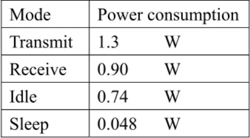
Table 1.1: Lucent WaveLAN Silver PC card power consumptions of all modes Mode Power consumption

Transmit 1.3 W Receive 0.90 W

Idle 0.74 W

Sleep 0.048 W

unavailable for transmit and receive. In other words, the node becomes deaf and dumb in the sleep mode. The longer a node stays in the sleep mode, the more power it saves. The Table 1.1 is the power consumptions in different modes on a Lucent IEEE 802.11 WaveLAN PC Silver card [6]. As the table lists, the power consumption of sleep mode is much smaller than other modes.

In 802.11 MAC, the Low-Power Mode [7] can operate only in the infrastructure network. This method shifts the responsibility of receiving the packets on mobile nodes to the base station. The base station has to keep the packets in a queue that should be received by those sleeping nodes. The sleeping nodes wake up periodically and take over the packets from the base station. The scheme has two disadvantages. First, the store space in the base station has to be enlarged for stocking the packets sent to sleeping nodes. Second, there has to be a special node such as base station to take over the tasks of other sleeping nodes. And this special node is not existed in the ad hoc network.

The power management scheme proposed by Kwon and Cho [7] is designed for ad hoc network. Each sleepy node should broadcast a SLEEP_IN message to inform its neighbors, and each active node should keep track on the states of neighbors. An awakening node sends the SLEEP_FIND to get the newest neighbor state information from other active node. This method distributes the responsibility of the base station to all active nodes. But there is still one limitation that a node can’t switch into sleep

(17)

state when it finds out that it has no active or idle neighbors. This node has to keep awake as the node state information maintainer. If the node is going into sleep, the other neighbor nodes cannot get any neighbor state information when they wake up. This limitation may cause some wasting power on the last active node.

The second category of the power saving algorithms is the active power saving category. In this area, the key feature is that the factors for an antenna to transmit a packet are adjustable. By adjusting of these factors, the power consumption during a transmission can be reduced. Therefore, the node can tune these factors to minimize the transmission power consumption and reach the goal of power saving.

We introduced two of these factors and the way how they save power: the modulation rate and the transmission power. Dynamic Modulation Scaling (DMS) [8] tunes the modulation rate as well as the consuming power. The modulation rate is the number of bits per symbol. Because the sending symbol number per second is fixed, the sending bit number per second decreases as the modulation rate decreases. The lower the modulation rate, the lower the transmission power consumption, but the higher the packet delay.

Transmission power control tries to minimize the transmitted signal power level, and so is the power consumption. Zhou and Nettles demarcate three power control schemes [9]: the strong transmit power, the weak transmit power, and the optimal transmit power. Strong transmit power (STP) is used as a no power saving scheme. It always maximizes the transmission power. Most portion of the power is wasted in small range transmission. Weak transmit power (WTP) is completely opposite to the STP. It tunes the transmission power to the minimum required value. WTP is the most successful scheme in reducing power consumption, but has the worst ability for against suddenly changes on channel state. This scheme can’t avoid contentions completely. The Optimal Transmit Power (OTP) MAC is proposed by Zhou and

(18)

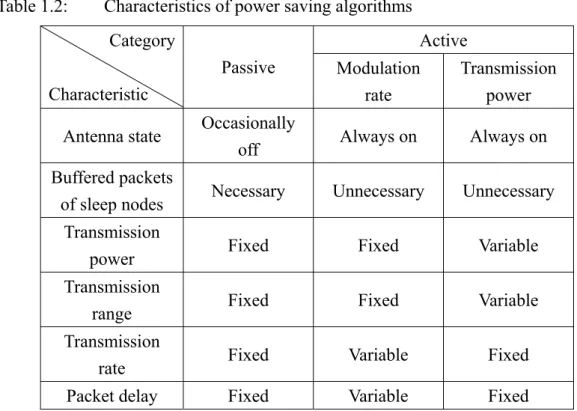
Table 1.2: Characteristics of power saving algorithms Active Category Characteristic Passive Modulation rate Transmission power Antenna state Occasionally

off Always on Always on Buffered packets

of sleep nodes Necessary Unnecessary Unnecessary Transmission

power Fixed Fixed Variable

Transmission

range Fixed Fixed Variable

Transmission

rate Fixed Variable Fixed

Packet delay Fixed Variable Fixed

Nettles [9]. It adjusts the transmission power to the minimum required power that can avoid all contentions and improves the disadvantage in WTP.

We compare the above mentioned methods and the result is shown in the Table 1.2.

1.4 Fair Scheduling Algorithms with Power Saving

Support

The algorithms combined power saving and fair scheduling are rarely to find. Following are three algorithms that are proposed to this domain.

1.4.1 Rate-Based Bulk Scheduling

Rate-Based Bulk Scheduling (RBS) service model [10] combines the passive power saving approach with SFQ. This algorithm works in the centralized structure network. The base station plays the role of scheduling the channel access among

(19)

mobile nodes. Mobile nodes that have no data to transmit or receive are going to sleep and minimize the consumption of power. The mainly task for the algorithm is to satisfy the minimum requirements of flows. As the goal is reached, it turns to conserve the power consumptions. When all flows have satisfied services, the scheduler then provide service to a flow concentrically until the buffer of that flow is cleaned up. The fully-served approach makes active nodes (either one of transmitter and receiver) to finish their job holus-bolus and expected to have a long sleep later. Thus, the transitions of node states can be reduced and so is the power consumed on transiting.

1.4.2 Energy Efficiency Weighted Fair Queuing

An energy efficiency version of WFQ is proposed on [8] and called E2WFQ. This algorithm puts the DMS mechanism on the original WFQ algorithm to save energy. It explains that the maximum transmission rate is not always necessary, especially when the input rate of a flow is lower than its service rate requirement. Therefore, the service rate can be reduced in some cases. The reduction of service rate can lead the transmission power consumption to be reduced. However, it also leads the packet delay to be increased. The packet delay is serious when the packet size is large or the service rate is quite small. The packet delay in low service rate could be ten times than that in the high service rate.

1.4.3 Channel State Dependent E

2

WFQ

Channel State Dependent E2WFQ [11], as known as CSDE2WFQ, is an improvement version of E2WFQ with the consideration of channel state. The channel state is assumed to be either good or bad. When the channel state is bad, the packet deliver probability is low. During the packet scheduling, the scheduler will check the

(20)

channel state of the selected packet. If the channel of the selected packet is bad, the transmission will delay for a while. The packet delay caused by the bad channel state is caught up by raising the service rate. In the ideal situation, this algorithm has the same packet delay guarantee as the E2WFQ. But for the packet that have to be sent with the maximum service rate, the delay of the bad channel has no way to be caught up.

1.5 Motivation

According to the introductions in previous sections, we find out that the above mentioned algorithms have their shortness. For the RBS algorithm, the bandwidth sharing for the satisfy flows may lead to seriously unfair. For the E2WFQ and CSDE2WFQ, the packet delay may be too long in the worst case. Therefore, we proposed a power saving fair queuing algorithm, called Start-time Fair Queuing with Power Saving (SFQ-PS) algorithm. We embed the active power saving approach of tuning transmission power into the fairness queuing algorithm, SFQ. The mainly idea of the combination is to break the packet selection of fairness queuing in the short term and replace it with a new packet selection which is focus on the power saving aspect. The factor of the power saving packet selection is defined according to the power saving approach above mentioned. Thus, in our system, we use the power saving approach in the bottom layer and put our proposed algorithm as the packet scheduler.

1.6 Thesis Organization

We illustrated the background in the Chapter 2. In Chapter 3, we proposed an algorithm, called Start-time Fair Queuing with Power Saving (SFQ-PS) algorithm, as

(21)

a combined algorithm of power saving and fair queuing. The simulation results are shown and discussed in the Chapter 4. The conclusion and future work are illustrated in the last chapter.

(22)

Chapter 2. Background

2.1 Propagation models

The power of a signal received by a receiver is always weaker than that sent by a transmitter. The reason is that when signals are propagated through the media, the power of signals will decrease as the transmission distance getting longer or the occurrence of obstacles, such as trees, walls, etc. The propagation models define how the signal fades due to the distance extending.

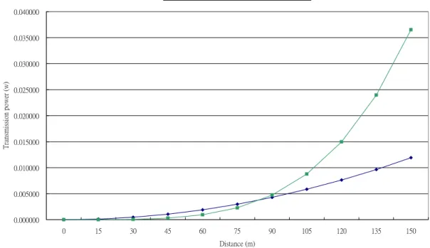
To have a detail understanding of the relation between transmission power and receipt power, we found the propagation models being most frequently used: the free space propagation model and the two-ray ground propagation model [9][12]. Due to

0.000000 0.005000 0.010000 0.015000 0.020000 0.025000 0.030000 0.035000 0.040000 0 15 30 45 60 75 90 105 120 135 150 Distance (m) Trans m is si on p ow er (w )

Free space model Two-ray ground model

Figure 2.1: The distance-transmission power curves of free space model and two-ray ground model

(23)

the oscillation from the combination of constructive part and destructive part of the two rays, the two-ray ground propagation model doesn’t have a good estimation in the short distance. Thus, we adopt the free space propagation model in the short distance, and the two-ray ground propagation model in the long distance. A reference distance is predefined to switch operating modes between these two models. If the distance is less than the reference distance, the free space propagation model is used. Otherwise, the two-way ground propagation model is more appropriate. The value of reference is defined as 87 m, which is the cross point that has almost the same results in these two models. The transmission power vs. distance of both models is drawn in the Fig. 2.1.

Assuming that the transmission power is , and the receipt power is . The distance between transmitter and receiver is d. The free space propagation model is defined as follows [9]: t P P_r

(

)

2 2 4 t t r r P G G P d λ π ⋅ ⋅ ⋅ = ⋅ ⋅ , (2-1)

where is the gain of transmit antenna, is the gain of receive antenna, and λ is the wave length.

t

G G_t

The two-way ground propagation model is defined as follows [9]:

2 2 4 t t r t r r P G G H H P d ⋅ ⋅ ⋅ ⋅ = , (2-2)

where and are the heights of the transmit antenna and receive antenna.

2

t

H H_t2

2.2 Receiving power criteria

There are two receivable signal thresholds in 802.11 MAC. The first one is the threshold of the power of receiving signal. Only the signals with power stronger than

(24)

that threshold can be received successfully. The threshold is given as 3.652．10-10 (W) and is defined as the minimum receivable power. We represent it with TH_rx.

The second threshold defined in 802.11 MAC is the capture threshold. The capture threshold, also known as signal-to-interference-and-noise ratio (SINR), is a threshold to make sure a receiver can decode signals from interferences correctly. The definition of SINR is [13]: ( ) r thermal MAI P SINR times P P = + . (2-3) r

P is the receipt power in receiver, P_thermal is the background noise power, and MAI

P is the multiple access interferences sent out by other nodes during receiving

period. With different measurement, we can transform the equation (2-3) in to following equation:

10

( ) 10 log ( ( ))

SINR dB = ⋅ SNR times . (2-4)

The minimum value of SNR in 802.11 MAC is defined as 10 dB [9], which means the receipt power must be at least 10 times larger than the summation of noise power and interference power.

The minimum required receipt power can be derived from above equations and represented into the equation:

max{ ,( ) ( )}

r rx thermal MAI

P = TH P +P ⋅SINR times (2-5)

Thus, we can calculate the requirement transmission power with the propagation model equations as long as the distance from the transmitter to the receiver is known.

2.3 Neighbor distance measurement

(25)

model. To calculate the distance with the propagation model equations, we have the information of the power of the receiving signal, also known as , with the support of the physical layer. Moreover, we know which frames that are requested to be transmitted with the maximum transmission power.

r P

With the information of the maximum transmission power and , we can estimate the distance easily from putting parameters into the propagation model equations.

r P

2.4 Calculations of Power Consumption

The power consumption in the transmit mode and the receipt mode can be written as [14]:

( )

_ _ ( ) r consume com rx t t consume t com tx com

t P P P P P P P P P P η = + ⎧ ⎪ ⎨ ₌ ₊ ₌ ₊ ⎪ ⎩ (2-6)

The common components that will work either in the transmit node or in the receipt mode, such as converter, base band processor, computing components, are considered to have the same power consumption in both modes. The common power consumption is assumed to be . The power consumption of the receiver front end that works only in the receipt mode is constant as . , the power consumption that drained by the power amplifier, is related to the transmission power and the power conservation efficiency

com P rx P Ptx t P

( )

Pt

η . η

( )

Pt is a function of that represent the

ratio of the signal power ( ) sent out by the antenna to the total power consumed ( ). t P t P tx P

(26)

2.5 Decision of the transmission power

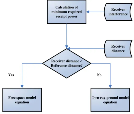
In this section, we illustrate the procedure of determining the transmission power in the transmitters. As the Fig. 2.2 shown, a transmitter has to know the receiver’s distance and interference. The information can be fetched in the previous transmissions. We have introduced the measurement of neighbor distance in the Sec. 2.4. With the information, the transmitter then calculates the minimum required receipt power with the receiving power criteria we introduced in the Sec. 2.3. After that, the minimum transmission power can be derived with the equation (2-1) (for free space model) or (2-2) (for two-ray ground model) that listed in the Sec. 2.2. Finally, the transmitter can determine the transmission power with the knowledge of the minimum transmission power. With the transmission power, the power consumption during the transmission can be calculated with the equation (2-6).

Receiver interference Calculation of minimum required receipt power Receiver distance < Reference distance?

Free space model equation

Two-ray ground model equation

Receiver distance

No Yes

(27)

Chapter 3. Start-time Fair Queuing with Power

Saving Algorithm

3.1 Characteristics

3.1.1 Distributed structure

This algorithm is based on the totally distributed structure. All the nodes have the responsibility of sending beacons periodically and receiving neighbors’ beacons. The most important purpose for the beacon exchanging procedure is to get the channel state information of neighbors, which is the source of the scheduling parameters for our algorithm. The other frames either control frames or data frames can also be referred for the updating of the neighbor distance.

3.1.2 Power awareness

The physical layer has the responsibility of detecting the powers of signals or interferences and m

3.2 Assumptions

We make following assumptions in our network model.

odifications are

2. it power approach with the original strong akes the power information available for the MAC layer. With the support of the physical layer, we can reach the goal of saving power with the knowledge of the power information.

1. In the MAC layer, the 802.11 MAC is adopted. No m made for this part.

(28)

transmit power approach in the 802.11. The control frames, such as RTS, CTS, ACK, and Beacon, are sent with the strong transmit power. The weak transmit power is used only in the transmission of DATA frame. The equations used for computing the minimum required power is discussed in later section.

There’s only one channe

3. l for transmission. Among various kinds of

4. hop transmission is available in this network.

3.3 Models

n ng sections, we present several models used in our algorithm and simu

3.3.1 Determination of the transmission power

A iver and P_r

is the minimum required receipt signal in order to against the noise and interferen channel errors, we only consider the error caused by collisions. The channel state is variable according the channel state model illustrated later.

Multi-5. No consideration of node mobility.

I the followi

lation. The transmission power model combines the original propagation models and the concept of the SINR. We illustrate the combination model in the Section 3.3.1. In Section 3.3.2, we introduce the energy model which represents the equations of the transmission and receipt power consumptions. This model can be used for the simulation of the energy variation. 3.4. Finally, the emulation of the background noise state is practiced in the help of the two-state Markov process which we will demonstrate in the last section.

ssuming that d is the distance between the transmitter and the rece

(29)

We can derive P_r with Equation (2-3).

From prop ation models and the ag SINR, we compute the transmission power with

itation of the antenna, P_t is bounded in

the Equation (2-1) and (2-2). Equation (2-1) is used in free space model as d is no larger than the reference distance. Other wise, equation (2-2) and two-way ground model are used.

To the lim

[

0,PMAX

]

. PMAX is the

maxi

3.3.2 Energy model

imulating the consuming of the energy during transmitting and r

n 2.2.4, we know that an energy model have the following param

tx g to the transm

t

mum power that an antenna can transmit. We use the equations above in the WTP mechanism in PHY layer and the computation of scheduling factors in our proposed algorithm.

For the purpose of s

eceiving, we have to determine the energy model that represents the variation of the power consumption.

According to sectio

eters: P_com, P_rx, and P_tx. The values of the P_com and P_rx are often assumed

to be invariant. The value of P have to calculated accordin ission power P and the power conservation efficiency

( )

. The former parameter is known trivially. The latter one can be represent with various kinds of mathematic formulas.

t

P

η

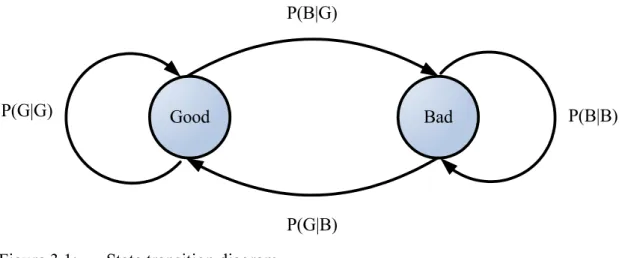
3.3.3 Background noise state model

The background noise state model represents the variation of the background noise state. With the help of the background odel, we can easily simulate the channel error

noise state m

(30)

P(B|G)

Good Bad

P(G|B)

P(B|B) P(G|G)

Figure 3.1: State transition diagram

ess, multi-state Markov Process, Gaussian mplitude distribution, and so on.

o background noise and the channel is almost clear exce

bability that jumps to another state, and the other probability that rema

air Queuing with Power Saving Algorithm

1. N ation Table (NIT)

This table records the states of neighbors. Each neighbor has an entry including the node ID, distance to the node, and interference over the node. The interference example, the two-state Markov Proc

a

Gilbert model is a two-state (Good and Bad) Markov Process model. When the state is in the Good state, there’s n

pt the interference generating by nodes. Otherwise, the background noise is large. The transmission in the Bad state has to resist both the node interferences and the background noise.

State transformation of the Gilbert model can be drawn as the Fig. 3.1. In each state, there is a pro

ins unchanged. We denote the probability to be P(X|Y) that the current state is X and the next state is Y.

3.4 Start-time F

3.4.1 Data structure

(31)

over node is got from the Beacons sent by neighbors. We assume that antennas can detec

eter is the threshold of the leading count. When there is a flow with leading count over the threshold, the flow is considered to be an over satisfied flow and the algorithm will freeze its right of sending packet. It has to wait until the t becomes smaller than the TH_LC. The larger value we given to this param

s are created by us.

1. St

igned a ST value as the finish tag of last incoming packet if the corresponding flow has queued packets. Otherwise, this value is assigned as the

e. The equation of ST can be written as followings:

t the signal power sending from neighbors and the distance can be derived with some simple calculations according to the Equation (2-1) and (2-2).

3.4.2 Tunable parameters

1. TH_LC This param

leading coun

eter, the more power saving scheme works and the less fairness guarantee.

3.4.3 Scheduling Parameters

Following are the parameters that our scheduling procedure base on. First two parameters are continued using from the SFQ algorithm. Other four parameter

art tag (ST)

The virtual time tag that used by SFQ to make packet selection decision. Each incoming packet is ass

system virtual tim

( )

{

1

}

max , k k k i i i S = F − V a . (3-1) 2. Finish tag (FT)

(32)

and the result o equation below:

f packet length divided by the flow weight. The FT is assigned by the

k k i i L S W = + . (3-2) 3. Virtual tim

Each node has a virtual time parameter that is equal to the start time tag of the serving pack his value will always be the same as the minimum start time tag over whole system. The detail process for maintaining this

k i F

i

where W_i is the weight of each flow i.

e (VT)

et. We made a little change that t

parameter is explained in the next section.

4. Channel state (CS)

Each flow in a node has its own CS. The equation of CS is defined as:

_ _ _ _

MAX

Pt current required Pt minimum required P

CS = − , (3-3)

0≤CS< , 1

required is the minimum required power for current

transm

any noise a arantees the

received power is e power. The

maxi

where Pt_current_

ission. Pt_minimum required_ is the required power for the case without

nd interference. Intuitively, it’s the required power that gu stronger than the threshold of the minimum receivabl

mum power that an antenna can use for transmitting is P_MAX. As we know,

_ _

Pt current required must be in the range of

[

Pt_minimum required P_ , MAX

]

.

(33)

5. Additional power consumption (APC)

It is the value to represent the ex consum packet at that time. We define the parameter as follow

_

tra ption of power for transmitting the equation:

APC=CS×packet size. 4)

alue of the additional transmission power vs. m representation of the transmission tim param ption that drained aw

mission of the packet with the minimum ST of whole node. A flow with non-zero LC is named to be as a leading flow. Otherwise, it up, the degree of fairness goes down. When the SFQ scheduling approach is com

(3-The CS parameter is the percentage v

aximum transmission power. In other words, it means how much additional energy is drained per unit time. We take the packet size as a

e, i.e. the time to consume power. Intuitively, the product of these two eters is the extra consumed power of the packet.

As the best situation of a channel, the CS is equal to zero and the APC is zero, too. In this case, no matter how long the packet is, it has the highest priority to be transmitted. When the channel is in the best case, additional power for competing with interferences is not necessary. Thus, the transmission power consum

ay is the minimum power consumption and all packets that can be transmitted with the minimum power consumption are encouraged to send. This is the reason why we ignore the effect of packet size in the best case. The priority of packet is higher as long as its APC is lower.

6. Leading count (LC)

Each flow has this parameter. It shows the amount bytes of size of the packets that are transmitted before the trans

is a non-leading flow. When the value goes

pletely followed, the leading counts of all flows keep zero all the way.

(34)

7. SENT

It’s a flag that indicate if the packet is already sent out. We use the flag to mark those packets that are sent out with breaking the rules of SFQ.

algorithm to a new sequence that consumes less transmission power than the original one. The algorithm can be separates as the following steps. Step 1 is the initial step for the system. Step 2, 3, and 4 are formed as a scheduling round that repeated continuously

ong the flows with LC smaller than the threshold TH_LC, The first unsent NT flag is down) that has the minimum ACP is selec

inimum one. If the number of fitting packets is lection goes following the rules of SFQ: select the one w

3.4.4 Proposed Algorithm

We propose the Start-time Fair Queuing with Power Saving (SFQ-PS) algorithm for the purpose of switching the sequence that scheduled by the original SFQ

. Step 3 and 4 are mutual steps for the packets selected from power saving consideration and those selected from fair scheduling consideration.

1. Initialization

At the beginning of the system, we set the values of all LCs to be zero. The virtual time is set to be zero, too.

2. Packet selection Am

packet (i.e. the first packet that SE

ted to be sent. If there are two or more suitable packets, we compare the LC among their flows and find out the m

still more than one, the packet se

ith the minimum ST. If the chosen packet is not the packet with the minimum ST, the virtual time won’t be updated to its ST.

3. Null packet insertion

(35)

the ST of the sent packet. If the sent packet has the minimum ST, we directly remove that packet and jump to the next step. Otherwise, at the flow of the sent packet, the LC is increased by the size of the sent packet. Moreover, we put a null packet that has the e t packet in its original location in the queue and mark the SEN

is null packet is selected. After this step, next round starts from

sam ST and FT as the sen

T flag of this null packet. Thus, the length of queue is not changed after this round. In this case, step 4 isn’t need and we directly stat next round from the step 2. 4. Minimum ST searching

In this step, we try to find out the packet with the minimum ST that is not sent out yet. The packets are selected in the increasing ST order, and the virtual time is modified to the start time tag of selected packet. If the SENT flag of the selected packet is set, we remove it from queue and decrease the LC of that queue by one. Th step keeps until the first

the second stop again.

3.5 Example

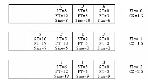
We explain the process with an easy example. Table 3.1 shows a sequence of incoming packet. When all the packets are received by the scheduler, the scheduler state becomes as the state graph drawn in the Fig. 3.2.

(36)

Table 3.1: Packet ID

Packet information of example

Flow ID Flow weight Packet size CS

A 0 2 6 1.5 B 0 2 10 1.5 C 0 2 8 1.5 D 1 1 2 1.5 E 1 1 3 1.5 F 1 1 5 1.5 G 1 1 7 1.5 H 2 3 9 2.5 I 2 3 9 2.5 J 2 3 18 2.5

T Scheduling process of example Round

Algorithm

0 1 2 3 4 able 3.2:

Flow N LC Next N L Next N LC ext N LC NeC N xt N LC Next

0 3 A 2 B 2 B 2 B 2 B 1 4 D 4 D 3 E 3 E 2 F SFQ 2 3 H 3 H 3 H 2 I 2 I 0 3 0 A 3 0 A 3 0 A 2 0 B 2 0 B 1 4 0 D 3 2 E 2 5 F 2 3 F 1 8 G SFQ-PS 2 3 0 H 3 0 H 3 0 H 3 0 H 3 0 H Round Algorithm 5 6 7 8 9

Flow N LC Next N L NextC N L NextC N L Next N LC NextC

0 1 C 1 C 1 C 1 C 0 1 2 F 2 F 1 G 1 G 1 G SFQ 2 2 I 1 J 1 J 0 0 0 1 10 C 1 0 C 0 8 0 8 0 8 1 1 8 G 1 5 G 1 5 G 1 0 G 0 7 SFQ-PS 2 3 0 H 2 0 I 2 0 I 1 0 J 1 0 J

(37)

For the packet selection of the SFQ, the start is the only tion ut in m, the APC, i.e. the production of the CS and the packet size is considered

first. The pa c i e b

packets of the flow remained in the queue. LC is the leading count value and Next is the next pack to nd n t q ue. he ac ts ith e me e ag e s lected in ea g rd o e fl I T am ter ar ssume o e unchanged in is am e d e lue of TH_LC is set to be 4.

tag considera . B our algorith

cket sele tion process s shown is th following ta le. N is the number of

et se i he ue T p ke w th sa tim t ar e the incr sin o er f th ir ow D. he CS par e s e a d t b

th ex pl . An th va

The packet selecting sequence of the SFQ is {A, D, H, E, B, I, F, J, C, G}, and the sequence of SFQ-PS is {D, E, A, F, B, H, C, I, G, J}. We can find out that due to Flow 1 has both smaller CS and smaller average packet size, the scheduler prefer the packet of this flow. For limiting the violation of the fairness, the scheduler turns to selecting other flows when Flow 1 has a LC that exceed the threshold TH_LC.

(38)

Chapter 4. Simulation and Results

In this chapter, we compare our proposed algorithm with original SFQ algorithm. The power adjustment mechanism works equally in both scenarios. Moreover, we compare the proposed algorithm with different value of tunable parameters.

4.1 Simulation environment

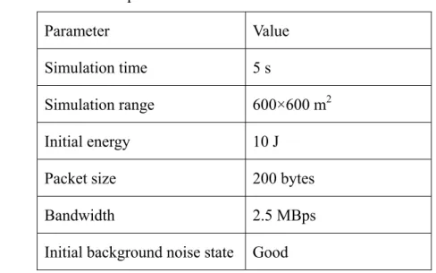
In our simulation, there are 10 nodes randomly distributed in a plain 600×600 m2. The initial energy of each node is 10 J. The packet size of all flows is set to be 200 Bytes. The generate rate of the constant-bit-rate (CBR) flow is 40KBps. The background noise state is assumed as good state at the beginning, i.e. there’s no background noise at first. The simulation parameters are listed in the Table 4.1.

Table 4.1: Simulation parameters

Parameter Value Simulation time 5 s

Simulation range 600×600 m2 Initial energy 10 J

Packet size 200 bytes

Bandwidth 2.5 MBps

(39)

4.2 Energy and Channel models

4.2.1 Energy model

The model of power consumption we use is following the model illustrated in [14][15]. P_com is set to be 0.5 watt. P_rx is set to be 0.05 watt. η

( )

P_t is defined as

an exponential curve. Thus, the ratio becomes higher when the transmission power consumption rises up. The function of η

( )

Pt is defined as below:

(

₍ ₎

)

_{0.02 5}15 t P t P dBm η = ⋅ (4-1)

The tunable power level is from -15dBm to 15dBm with 1dBm gaps. 31.623 mW is the maximum transmission power related to 15 dBm and the corresponding minimum transmission power to -15 dBm is 0.0316 mW. The maximum transmission range is about 145 m.

4.2.2 Background noise state model

We use the Gilbert model [11] as our background noise state model. The background noise N is 0 W in the Good state and is set to be 3.652×10-10 W in the Bad state. The probabilities of state transitions are given with different values for the simulations.

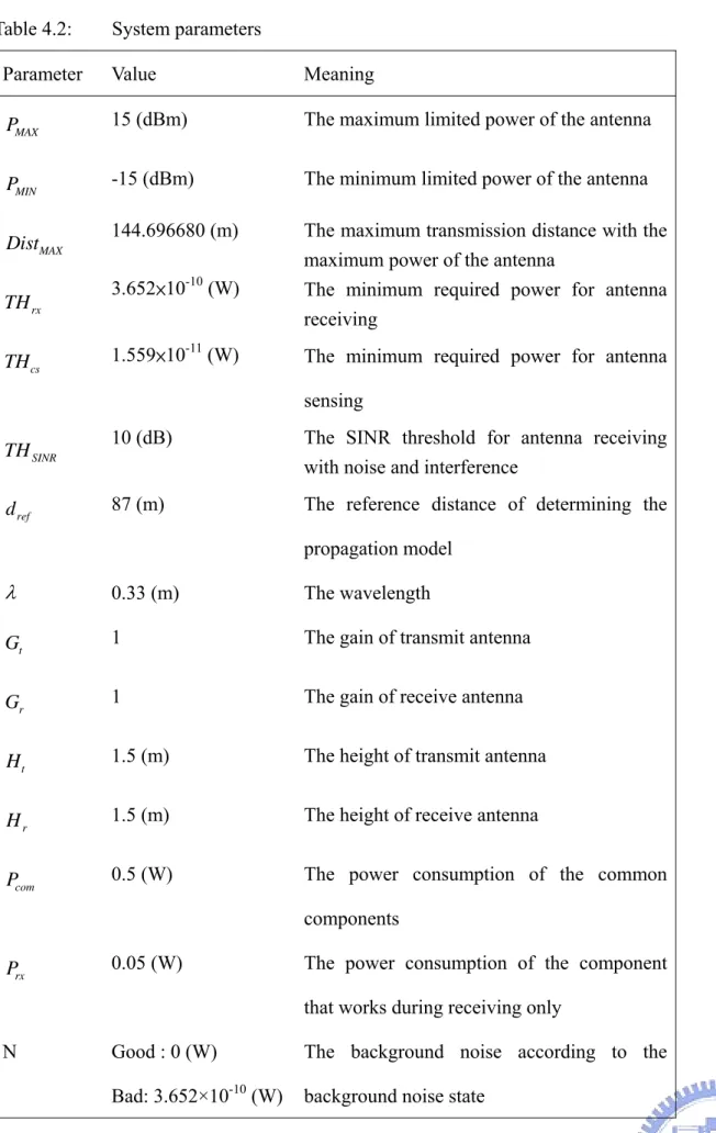
4.3 System Parameters

The system parameters and their values are listed in the following table. These parameters appear in the equations of the transmission power and the energy model. The computation of several scheduling parameters is based on them, too.

(40)

Table 4.2: System parameters

Parameter Value Meaning

MAX

P 15 (dBm) The maximum limited power of the antenna MIN

P -15 (dBm) The minimum limited power of the antenna MAX

Dist 144.696680 (m) The maximum transmission distance with the

maximum power of the antenna

rx

TH 3.652×10

-10_(W)

The minimum required power for antenna receiving

cs

TH 1.559×10-11 (W) The minimum required power for antenna

sensing

SINR

TH 10 (dB) The SINR threshold for antenna receiving

with noise and interference

ref

d 87 (m) The reference distance of determining the

propagation model

λ 0.33 (m) The wavelength

t

G 1 The gain of transmit antenna r

G 1 The gain of receive antenna

t

H 1.5 (m) The height of transmit antenna r

H 1.5 (m) The height of receive antenna com

P 0.5 (W) The power consumption of the common

components

rx

P 0.05 (W) The power consumption of the component

that works during receiving only N Good : 0 (W)

Bad: 3.652×10-10 (W)

The background noise according to the background noise state

(41)

4.4 Performance metrics

1. Power consumption: the metric is measured as the average transmission power consumption per packet. We get the metric by dividing the summation of transmission power consumption of all nodes with the amount of successful end-to-end packet deliveries.

2. Network life: we define this metric to the life time of the first dead node. It’s an important metric for determine the performance of power saving. The longer the network life, the more power saved.

3. Fairness index: assume that each flow i has a weight . According to the

fairness based on throughput in [16], we define our fairness index as the following equation: i W 2 1 2 1 _ n i i i n i i i T W fairness index T n W = = ⎧ ⎫ ⎨ ⎬ ⎩ ⎭ = ⎧ _⎛ _⎞ ⎫ ⎪ ⎪ ⎨ ⎜ ⎟ ⎬ ⎝ ⎠ ⎪ ⎪ ⎩ ⎭

∑

(4-2)

n is the number of flows in the system. is the throughput of each flow i. The

range of this equation is in

i T

]

(

0,1 . The fairness is better when the result is closer to one.

4. Packet drop rate: the ratio of packet that sent out by flows but not received until the end of simulation. We compute the metric with the following formula:

SENT RECEIVED SENT Packet Packet Packet − . (4-3)

(42)

state get worse, the packet drop rate will rise up.

5. Throughput: the amount of delivery data in the unit time. We calculate the successful delivery bytes in one second as the throughput. This metric is affected by the channel state condition, too.

6. Packet delay: the time spent for a packet to be sent from source until receiving by the destination, including the time spent for packet retransmission.

4.5 Simulation results

We simulate the above mentioned metrics and the results are shown in the following sections. The weak transmission power (WTP) is chosen as our transmission power mechanism. We compare the original SFQ and our proposed SFQ-PS of different TH_LC values: 1000, 2000, and 3000 bytes.

There are two scenarios. In Scenario one, we fixed the background noise appearance probability to P(G|B) = 0.02 and P(B|G) = 0.08. We generate 6 to 14 CBR multihop flows with constant packet generate rate 40KBps. The flow weights are randomly assigned in the range of

[ ]

1,3 . The sources and destinations of these flows are randomly selected. In Scenario two, we use 10 CBR multihop flows with packet generate rate 40KBps. The flow weights are randomly assigned in the range of

[ ]

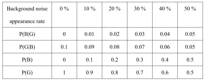
1,3 . The sources and destinations of these flows are randomly selected. The background noise state transition probabilities P(G|B) and P(B|G) are given as Table 4.3.

(43)

Table 4.3: Background noise appearance rate setting of scenario two Background noise appearance rate 0 % 10 % 20 % 30 % 40 % 50 % P(B|G) 0 0.01 0.02 0.03 0.04 0.05 P(G|B) 0.1 0.09 0.08 0.07 0.06 0.05 P(B) 0 0.1 0.2 0.3 0.4 0.5 P(G) 1 0.9 0.8 0.7 0.6 0.5

The relation of P(G|B), P(B|G), P(B), and P(G) can be derived from the following equations: ( | ) ( | ) 1 ( ) ( ) 1 ( ) ( | ) ( ) ( | ) ( ) P G B P B B P B P G P B P B G P G P B B P B + = ⎧ ⎪ ₊ ₌ ⎨ ⎪ ₌ ₊ ⎩ ( | ) ( ) ( | ) ( | ) P B G P B P B G P G B ⇒ = + (4-4) ( | ) ( ) 1 ( ) ( | ) ( | ) P G B P G P B P B G P G B = − = + (4-5)

(44)

4.5.1 Scenario one

In the Scenario one, we observe the variation of metrics according to different flow numbers 6 ~ 14.

4.5.1.1 Power consumption

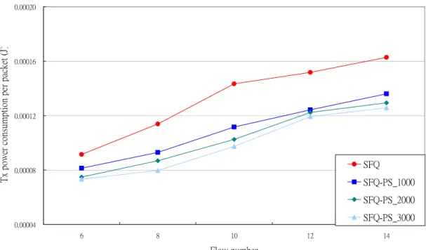
The power consumption reflects the ability of power saving. The less the power consumption, the more powerful the ability of power saving. We observe this metric in the viewpoint: the transmission power consumption per packet, which the packet means those packets that are successful delivered from a sender to a receiver.

The Fig. 4.1 shows the transmission power consumption per packet. The transmission power consumption increases when the flow number becomes more. As the flow number increase, the traffic load becomes heavy, and the collisions happens more often. Thus, the power consumption of retransmitting packets increases. The average transmission power consumption of packets increases, too.

0.00004 0.00008 0.00012 0.00016 0.00020 6 8 10 12 14 Flow number Tx p ow er con su mption per pac ke t (J ) SFQ SFQ-PS_1000 SFQ-PS_2000 SFQ-PS_3000

(45)

The power consumption of packet in our proposed algorithm with the WTP mechanism is less than that in SFQ. As the TH_LC rises up, the power consumption decreases. This is because the probability of selecting a packet according to the channel state rather than the fair queuing rules is higher.

4.5.1.2 Network life

The network life is another metric for representing the ability of power saving. As the network life is longer, the power saving ability is higher. We observed the dead time of the first node as the network life. As the Fig. 4.2 shown, the network life decreases as the flow number increases. That is, the increasing of flow number means the increasing of traffic load. Therefore, each node has to send more packets in a unit time, and the power consumes more quickly.

With the larger value of TH_LC in SFQ-PS, the network life is prolonged. Intuitively, the small power consumption of SFQ-PS results the long network life. With the raising of the TH_LC, the network life of SFQ-PS is extended.

20 25 30 35 40 45 6 8 10 12 14 Flow number N et w or k lif e (s ) SFQ SFQ-PS_1000 SFQ-PS_2000 SFQ-PS_3000

(46)

4.5.1.3 Fairness index

The result of fairness index is shown in Fig. 4.3. A higher fairness index means a higher guarantee of fairness. The fairness index goes down when the flow number increases.

For SFQ-PS with different TH_LC values, the fairness index is lower as the TH_LC is higher. The reason is that the packet selection with higher TH_LC obeys the power saving algorithm more often than the fair queuing algorithm. Therefore, the fairness index of SFQ-PS with larger TH_LC is smaller. As the flow number becomes larger, the fairness is hard to be guaranteed. Thus, the fairness indices of all algorithms become close.

0.50 0.60 0.70 0.80 0.90 1.00 6 8 10 12 14 Flow number F airness in dex SFQ SFQ-PS_1000 SFQ-PS_2000 SFQ-PS_3000

(47)

4.5.1.4 Packet drop rate

The packet drop rate shows how often the failure of the transmission. As the Fig. 4.4 shown, the packet drop rates increases following the flow number. With the increasing of flow number, the collisions happen more often. Thus, more packets are dropped due to the collision. As to the packets dropped at the end of simulation it also increases with the increasing collisions. Intuitively, more collisions make the packets stay in the queue much longer. Because the packet generating rate is stable, the number of queued packets increases as time goes by. Thus, the number of packets dropped at the end of simulation also increases with the increasing of flow number.

0% 10% 20% 30% 40% 50% 6 8 10 12 14 Flow number P ack et d ro p ra te ( %) SFQ SFQ-PS_1000 SFQ-PS_2000 SFQ-PS_3000

(48)

The improvement of packet drop rate in our algorithm can be ascribed to the part of selecting packet according to the transmission power consumption. The channel state is one of the factors we put in the power consumption consideration. As the traffic goes up, the probability of collision raise up. And the benefit of the consideration of channel state decreases.

4.5.1.5 Throughput

The throughput shows the average delivery amount of data. As the Fig. 4.5 shown, the performance of throughput decreases with the flow number increases. The reason is the same as previous section. As the flow number increases, the collisions happen more often. Thus, fewer packets are successfully delivered due to the collision and the throughput is dropped.

10000 15000 20000 25000 30000 35000 40000 6 8 10 12 14 Flow number T hroug hp ut (by te s/ s) SFQ SFQ-PS_1000 SFQ-PS_2000 SFQ-PS_3000

(49)

4.5.1.6 Packet delay

The packet delay shows how long does a packet take from the source to the destination. As the Fig. 4.6 shown, the packet delay increases following the flow number. With the increasing appearances of collision, the retransmission of a packet also increases. Thus, the time spent on failure transmissions is increased and so is the packet delay. 0.0 0.4 0.8 1.2 1.6 2.0 6 8 10 12 14 Flow number P ack et d el ay ( s) SFQ SFQ-PS_1000 SFQ-PS_2000 SFQ-PS_3000

(50)

4.5.2 Scenario two

In this scenario, we observed the effect of different background noise appearance rates to these four metrics. We tune the background noise appearance rate from 0% to 50%.

4.5.2.1 Power consumption

The transmission power consumption per packet is chosen as the power consumption metric we observed.

Fig. 4.7 shows the relation between the background noise appearance rate and the transmission power consumption per packet. We shows the background noise appearance rate as the value of P(B). As the background noise appearance rate goes up, the transmission power consumption increases. For the SFQ-PS algorithm, the power consumption is less when the ability of power saving is stronger, i.e. the TH_LC is higher. 0.00000 0.00010 0.00020 0.00030 0.00040 0 10 20 30 40 50

Background noise appearance rate (%)

Tx p ow er c on su m ptio n pe r pa ck et ( J) SFQ SFQ-PS_1000 SFQ-PS_2000 SFQ-PS_3000

(51)

4.5.2.2 Network life

The following figure shows the variation of network life in different background noise appearance rates. The network life decreases smoothly. For the case of low background noise appearance rate, SFQ-PS indeed prolongs the network life for about eight second.

Due to the large rate of background noise appearance, the power saving ability of SFQ-PS is shrinking. Thus, the network life difference between SFQ and SFQ-PS at the highly background noise appearance rate is quite small.

For the case of higher background noise appearance rate, the transmission power consumption per packet of SFQ-PS is lower than SFQ, but the packet deliver rate of SFQ-PS is higher than SFQ. Thus, the total power consumption, i.e. the product of transmission power consumption and the number of successful delivered packet, of both algorithms are almost the same. And the network life performances are almost the same. 0 20 40 60 80 100 0 10 20 30 40 50

N etw ork life ( s) SFQ SFQ-PS_1000 SFQ-PS_2000 SFQ-PS_3000

(52)

4.5.2.3 Fairness index

The result of fairness index with variation of background noise appearance rate is shown in Fig. 4.9. The background noise appearance rate largely affects the fairness index.

As the following figure shown, the fairness index difference of SFQ and SFQ-PS I is increased as the background noise appearance rate increased. That is, when the background noise appearance rate is bigger, the power saving part of our algorithm works longer. Comparing to the Fig. 4.7, the power consumption difference is also increased as the background noise appearance rate increased.

0.30 0.40 0.50 0.60 0.70 0.80 0.90 0 10 20 30 40 50

F airness in dex SFQ SFQ-PS_1000 SFQ-PS_2000 SFQ-PS_3000

(53)

4.5.2.4 Packet drop rate

The relation of background noise appearance rate and packer drop rate is shown at following figure. Due to the channel state is one of the factors we put in the power consumption consideration. The packet drop rate of SFQ-PS is reduced comparing to SFQ. The difference between SFQ and SFQ-PS shrinks as the background noise appearance rate raise up. It is cause by the increasing of background noise appearance rate. As the background noise appearance rate raise up, the channel state varies frequently, and the benefit of prediction of the channel state decreases. Therefore, the difference of performances shrinks to only 1%.

0% 10% 20% 30% 40% 50% 60% 70% 0 10 20 30 40 50

P ack et d ro p ra te ( %) SFQ SFQ-PS_1000 SFQ-PS_2000 SFQ-PS_3000

(54)

4.5.2.5 Throughput

The following figure shows the variation of throughput with the increasing of background noise appearance rate. The throughput of SFQ-PS is increased comparing to SFQ. The performance decreases with the increasing of background noise appearance rate. As the background noise appearance rate raise up, the packer drop rate raises up. Thus, the throughput drops down.

5000 15000 25000 35000 45000 0 10 20 30 40 50

T hroug hp ut (by te s/ s) SFQ SFQ-PS_1000 SFQ-PS_2000 SFQ-PS_3000

(55)

4.5.2.6 Packet delay

As the Fig. 4.12 shown, the packet delay increases following the background noise appearance rate. The frequency of collision increases as the background noise appearance rate increases. With the increasing appearances of collision, the retransmission of a packet also increases. The packet delay we calculate includes the time spent for transmission and retransmission. In other words, the packet delay is large if the retransmission is frequent. Thus, the packet delay increases with the increasing background noise appearance rate.

0.0 0.2 0.4 0.6 0.8 1.0 0 10 20 30 40 50

P ack et d el ay ( s) SFQ SFQ-PS_1000 SFQ-PS_2000 SFQ-PS_3000

(56)

Chapter 5. Conclusion and Future work

5.1 Conclusion

Energy is a scarce resource in the ad hoc network. The life time of mobile nodes can be enlarged as long as the algorithms implemented on them put a little effort on reducing the power consumption. In recent research, most of the algorithms for transmission power control don’t discuss the relation of transmission power and power consumption during transmission. And not much power saving considered algorithms are proposed in the fair scheduling domain, especially base on the transmission power control mechanism.

In the thesis, we proposed a scheduling algorithm that combines the issues of fair scheduling and power saving. Our mechanism works based on the idea of trading the short term fairness with the power consumption. We implement the thought by reform the SFQ algorithm. We compare our proposed algorithm with SFQ in the mechanism of weak transmission power.

With the result of simulation, the performance of our proposed algorithm is better in the transmission power consumption, network life, and packet drop rate. For the fairness, the SFQ-PS and SFQ perform similar. Thus, the SFQ-PS algorithm can reduce the transmission power consumption when the fairness remains almost the same.

(57)

5.2 Future work

In this paper, we make a casual decision of the routing protocol. The mechanism of routing protocol may improve or deteriorate the performance. We are going to compare the performance difference between several routing protocols. We’ll focus on the routing protocol that is designed for the least power consumption path selection.

Due to the lack of efficiency routing protocol, there’s no routing repair mechanism when the link between two nodes is broken. The effect to the broken links caused by the no power node won’t work. Thus, we make the observation of network life to only one node draining out of energy. As the join of routing repair mechanism, the power consuming rate of active nodes will increase following from the increasing of dead nodes.

Another assumption we made is the ignorance of the node mobility, which is an important issue in ad hoc network. We will join the influence of mobility and improve the algorithm in such environment.